| Issue |
A&A
Volume 502, Number 1, July IV 2009
|
|
|---|---|---|
| Page(s) | 325 - 332 | |
| Section | The Sun | |
| DOI | https://doi.org/10.1051/0004-6361/200911738 | |
| Published online | 04 June 2009 | |
Scattering of solar energetic electrons in interplanetary space
C. Vocks - G. Mann
Astrophysikalisches Institut Potsdam, An der Sternwarte 16, 14482 Potsdam, Germany
Received 27 January 2009 / Accepted 22 April 2009
Abstract
Context. Solar energetic electrons are observed to arrive between 10 and 30 min later at 1 AU compared to the expectation based on their production in a solar flare and the travel time along the Parker spiral. Both a delayed release of electrons from the Sun and scattering of the electrons along their path are discussed as possible underlying mechanisms.
Aims. We investigate to what extent scattering of energetic electrons in interplanetary space influences the arrival times of electrons at a solar distance of 1 AU, as a function of electron energy and for different scattering models.
Methods. A kinetic model for electrons in interplanetary space is used to study the propagation of solar-flare electrons injected into the corona. The electrons are scattered by resonant interaction with a whistler-wave spectrum that is based on observed magnetic field fluctuation spectra in the solar wind. The arrival times of the electrons at 1 AU is determined by the electron flux exceeding a given threshold value.
Results. The simulation results show a significant influence of the scattering on electron arrival times. Electrons with energies in the range of several tens of keV are delayed by up to about one minute for a pure pitch-angle scattering model. It is demonstrated that this simplification is not applicable, and the full quasi-linear diffusion equation needs to be considered. This reduces the delays to values below 30 s.
Conclusions. It follows from these numerical studies that scattering of electrons in interplanetary space due to resonant interaction with whistler waves cannot explain the observed delays of 600 s, unless an unrealistic wave spectrum is assumed in interplanetary space.
Key words: scattering - waves - Sun: flares - Sun: particle emission - Sun: solar wind
1 Introduction
Solar flares are well known as generating high fluxes of energetic electrons. These electrons lead to the emission of radio waves as they traverse the background plasma of the solar corona, and release X-rays through bremsstrahlung and thermal emission when they are stopped by the ambient medium. But solar energetic electrons can also escape from the solar corona into interplanetary space, where they are directly observed by spacecraft (Lin 1974). Since electrons with higher energies move with higher speeds, they arrive earlier at the observer than those with lower energies. This velocity dispersion provides the opportunity to infer electron release times and travel path lengths from energy-dependent electron arrival times as registered by spacecraft (Krucker et al. 1999; Classen et al. 2003).Such an analysis is typically based on the assumption that the electron movement in interplanetary space is scatter-free. This assumption usually seems to work well, e.g. the electron travel times in Classen et al. (2003) are found to be inversely proportional to the electron speed.
However, substantial time differences frequently are found between the electron release times that are inferred from velocity-dispersion observations and the onset of X-ray and radio emission that indicates the presence of energetic electrons in the solar corona (e.g. Krucker et al. 2007; Haggerty & Roelof 2002; Klassen et al. 2002). The release of energetic electrons into interplanetary space seems to be delayed by from 10 min to 30 min.
This raises the question of whether the energetic electrons in interplanetary space belong to the same population that leads to coronal X-ray and radio emission in the solar corona, and if so, whether they are stored in the solar corona prior to their release, or if they are delayed due to scattering in interplanetary space. Cane (2003) presents interplanetary type III radio burst observations and argues that the electrons are delayed in interplanetary space, while Klein et al. (2005) come to the conclusion that the origin of delayed electron releases is the interplay between electron acceleration and injection into different magnetic structures in the solar corona.
The question of to what extent scattering of energetic electrons in interplanetary space can influence their arrival times at a solar distance of 1 AU has motivated the numerical study presented here. If the scattering modifies the arrival times significantly, this might lead to severe errors in the path lengths and release times as yielded by a simple velocity-dispersion analysis.
In the model presented in this paper, energetic electrons in interplanetary space are scattered through resonant interaction with electron cyclotron/whistler waves. The numerical model is based on solving the Boltzmann-Vlasov equation, including quasilinear-theory Fokker-Planck type equations for both wave-electron interaction and Coulomb collisions. The propagation of solar flare electrons in the model heliosphere after their release in the corona is studied. Electron arrival at 1 AU is defined as an increase of the spectral electron flux above a given threshold. This approach is complementary to Monte-Carlo simulations, like those of Agueda et al. (2005), who study the influence of interplanetary scattering on time-intensity profiles as recorded by spacecraft.
The paper is organized as follows. In the next section, the kinetic model is presented with emphasis on the resonant interaction between electrons and whistler waves in interplanetary space. Then, numerical results are presented, and their dependence on model assumptions is discussed. The paper closes with the conclusions and summary section.
2 The kinetic model
The kinetic model for electrons in the solar corona and in interplanetary space that is used here for a study of the propagation of flare-generated energetic electrons has been adopted from Vocks et al. (2008). This model is capable of handling relativistic electron energies and includes the effects of the inhomogeneous background plasma, Coulomb collisions, and resonant interaction between electrons and whistler waves. Its basic features are repeated here.
The kinetic model is based on solving the Boltzmann-Vlasov equation
that describes the temporal evolution of the electron velocity distribution function (VDF),
The Coulomb collisions are described by a Fokker-Planck equation that is based on the Landau collision integral (Ljepojevic & Burgess 1990). The Coulomb collision frequency is proportional to the background electron and proton number density, thus Coulomb collisions are most important in the relatively dense corona, and less in the tenuous solar wind where most of the electron scattering due to interaction with whistler waves happens. Under typical solar wind conditions, even thermal electrons have collisional mean free paths of the order of 1 AU. Coulomb collisions are calculated for all energies, although the collision frequency decreases with electron speed, v, as v-3, so that the energetic electrons released by a solar flare, with energies of several 10 keV, are essentially collisionless in the corona, and even more so in the solar wind.
But ignoring the Coulomb interaction beyond a given energy or below some minimum density would introduce a discontinuity into the model, that might lead to artifacts in the model results.
The interaction between whistler waves and electrons is described in more detail in the next sub-section. In order to provide the kinetic model with parameters for Coulomb collisions of the electrons with both electrons and protons, as well as for the whistler wave dispersion relation and the charge-separation electric field, a solar wind background model is needed. Such a model has to provide the magnetic field, densities and temperatures of electrons and protons, and the plasma flow speed, all as functions of the solar radial distance.
We have re-used the solar wind model of Vocks et al. (2005) that
describes the plasma conditions in a solar coronal funnel and in the fast
solar wind. The interplanetary magnetic field geometry of a Parker spiral is
also taken into account, based on an average solar wind speed of
![]() in interplanetary space.
in interplanetary space.
The Boltzmann-Vlasov Eq. (1) depends on three spatial
and on three momentum coordinates. For a simulation box with a spatial extent
from the solar corona over a few AU into interplanetary space, and with an
electron energy range up to the order of 100 keV with a resolution of less
than one electron thermal energy for lower energies, this cannot be solved
numerically. The computer costs would be excessive. The assumption of a
gyrotropic electron VDF not only eliminates one of the momentum coordinates,
namely the phase angle of the gyromotion, but also reduces the spatial
coordinates to a single coordinate, s, along the background magnetic field,
![]() .
In momentum space, the absolute value of the momentum, p, and the
pitch-angle,
.
In momentum space, the absolute value of the momentum, p, and the
pitch-angle, ![]() ,
are used as the remaining coordinates.
,
are used as the remaining coordinates.
2.1 Resonant interaction between electrons and whistler waves
The resonant interaction between electrons and whistler waves is described within the framework of quasilinear theory (Kennel & Engelman 1966). Only waves propagating parallel to the background magnetic field are considered here. The inclusion of obliquely propagating waves into the model would lead to highly complicated integrals over wave-vector space (Marsch & Tu 2001) with prohibitive computer costs. This simplification seems to be justified, since Bieber et al. (1994) have found that scattering of energetic particles in interplanetary space is mainly caused by parallel waves, while highly oblique waves contribute very little to it.
The quasilinear diffusion equation can then be written in the form given by
Marsch (1998), that reads in coordinates
![]() :
:
![$\displaystyle \left(\frac{\delta f}{\delta t}\right)_{\rm wh.} =
\frac{1}{p^2 \...
...l p} +
\alpha_{\theta\theta} \frac{\partial f}{\partial \theta} \right) \right]$](/articles/aa/full_html/2009/28/aa11738-09/img18.png)
with the parameters
with the whistler wave phase speed,
![]() ,
the electron speed,
,
the electron speed,
![]() ,
and the ``collision frequency'' associated with the
whistler-electron interaction:
,
and the ``collision frequency'' associated with the
whistler-electron interaction:
The main effect of the resonant interaction with plasma waves on the electrons is pitch-angle diffusion in the wave frame, leading to the formation of ``kinetic shells'' as described by Isenberg et al. (2001).
The frequency of a wave that interacts with an electron with given
momentum
![]() is determined by the resonance condition
is determined by the resonance condition
The maximum phase speed for whistler waves is half the electron Alfvén
speed,
![]() ,
with
,
with ![]() and
and ![]() being
the electron number density and mass, respectively.
In the solar wind, whistler wave phase speeds are typically of the order
of
being
the electron number density and mass, respectively.
In the solar wind, whistler wave phase speeds are typically of the order
of
![]() and are thus comparable to electron thermal
speeds. For energetic electrons with speeds that are a substantial fraction of
the light speed, c, pitch-angle scattering in the wave frame hardly differs
from pitch-angle scattering in the plasma frame. The coefficient
and are thus comparable to electron thermal
speeds. For energetic electrons with speeds that are a substantial fraction of
the light speed, c, pitch-angle scattering in the wave frame hardly differs
from pitch-angle scattering in the plasma frame. The coefficient
![]() then dominates the diffusion
Eq. (2). This has motivated the simulation run with pure
pitch-angle scattering that is presented in the results section of this paper.
then dominates the diffusion
Eq. (2). This has motivated the simulation run with pure
pitch-angle scattering that is presented in the results section of this paper.
2.2 Whistler waves in interplanetary space
The plasma wave spectrum in interplanetary space has been adopted from the earlier kinetic studies of Vocks et al. (2005), where the formation of the strahl and halo suprathermal electron populations in the solar wind have been studied. Unlike that paper, and the coronal loop model of Vocks et al. (2008), there are no additional whistler waves being emitted into the simulation box at the lower border in the computations presented here.
The wave spectrum in these models is based on a global spectrum of solar wind
electromagnetic fluctuations (Salem 2000), that is a compilation of
data from different instruments onboard the WIND spacecraft (Mangeney
et al. 2001). The ratio of the total wave power to the
background magnetic field energy density,
![]() ,
is of the order
10-3. Only a minor fraction of 1% of the total wave power
is assigned to whistler waves propagating parallel to the background
magnetic field, either sunwards or anti-sunwards. The rest of the wave power
can be in other wave modes, propagating parallel or perpendicular to the
background magnetic field, or obliquely to
,
is of the order
10-3. Only a minor fraction of 1% of the total wave power
is assigned to whistler waves propagating parallel to the background
magnetic field, either sunwards or anti-sunwards. The rest of the wave power
can be in other wave modes, propagating parallel or perpendicular to the
background magnetic field, or obliquely to ![]() .
.
As in Vocks et al. (2005), the proportion of the whistler waves
of the total wave power rises to 50% above the lower hybrid frequency,
![]() .
The reason for this is that in the solar wind, the plasma
frequency,
.
The reason for this is that in the solar wind, the plasma
frequency,
![]() ,
is much higher than the electron cyclotron frequency,
,
is much higher than the electron cyclotron frequency,
![]() .
This has the consequence that only whistlers can propagate
in the frequency range
.
This has the consequence that only whistlers can propagate
in the frequency range
![]() .
But for the energetic
electrons studied in this paper, resonance frequencies are well below the lower
hybrid frequency, so that this model assumption is not relevant here.
.
But for the energetic
electrons studied in this paper, resonance frequencies are well below the lower
hybrid frequency, so that this model assumption is not relevant here.
The diffusion Eq. (2) provides an estimate of electron mean free paths. For solar energetic electrons with energies of several 10 keV they are typically of the order 0.8 AU. Thus, they can be expected to be delayed by a substantial fraction of the free-propagation time from the Sun to 1 AU, which is e.g. 1250 s for 40 keV electrons. So delays by several minutes seem to be possible.
2.3 Solar flare electrons
The lower boundary of the simulation box is located in the corona,
with electron density,
The injection of solar flare electrons into the simulation box is done by modifying this lower boundary condition. The flare electrons have a power-law distribution whose parameters are derived from RHESSI observations.
The total number density of flare energetic electrons,
![]() ,
propagating downwards from the flare site can be derived by dividing the
electron flux distribution, which is obtained from hard X-ray (HXR) spectra,
by the the electron speed and the area of the thick-target interaction,
i.e. the HXR footpoint area, and integrating over all electron energies. Using
RHESSI (Lin et al. 2003) data, Holman et al. (2003)
have obtained values of the order of
,
propagating downwards from the flare site can be derived by dividing the
electron flux distribution, which is obtained from hard X-ray (HXR) spectra,
by the the electron speed and the area of the thick-target interaction,
i.e. the HXR footpoint area, and integrating over all electron energies. Using
RHESSI (Lin et al. 2003) data, Holman et al. (2003)
have obtained values of the order of
![]() for the peak of an X-class flare. Krucker et
al. (2007) have shown that the total number of electrons
injected into interplanetary space is just a small fraction of the
HXR-producing ones - 0.2% on average. We thus adopt a value of
for the peak of an X-class flare. Krucker et
al. (2007) have shown that the total number of electrons
injected into interplanetary space is just a small fraction of the
HXR-producing ones - 0.2% on average. We thus adopt a value of
![]() ,
which reflects the density of electrons propagating
outwards in a medium-sized flare.
,
which reflects the density of electrons propagating
outwards in a medium-sized flare.
We have chosen ![]() as a representative spectral index of the
accelerated electron flux (cf. Krucker et al. 2007; Warmuth
et al. 2009). Both rise and fall times of the electron injection
profile were taken as 1 min, which is a typical value both for HXR pulses and
type III radio bursts (cf. Fig. 1 in Krucker et al. (2007)). The
flare electron distribution has a low-energy cutoff at
as a representative spectral index of the
accelerated electron flux (cf. Krucker et al. 2007; Warmuth
et al. 2009). Both rise and fall times of the electron injection
profile were taken as 1 min, which is a typical value both for HXR pulses and
type III radio bursts (cf. Fig. 1 in Krucker et al. (2007)). The
flare electron distribution has a low-energy cutoff at
![]() ,
below which the distribution is constant.
,
below which the distribution is constant.
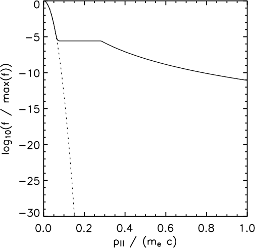 |
Figure 1:
Cut along the line
|
| Open with DEXTER | |
Figure 1 shows the lower boundary condition during the solar
flare. Note that the half-space
![]() is not relevant here, since these
electrons do not enter the simulation box. At low energies, the VDF is
dominated by the Maxwellian, or here
is not relevant here, since these
electrons do not enter the simulation box. At low energies, the VDF is
dominated by the Maxwellian, or here
![]() ,
distribution of the
coronal background plasma.
,
distribution of the
coronal background plasma.
As these energetic electrons propagate into interplanetary space after the onset of the flare, more energetic, i.e. faster, electrons will outpace the slower ones. The earlier arrival of more energetic electrons at some distance from the Sun has the consequence that the electron VDF there can become unstable to the generation of Langmuir waves, which eventually leads to the emission of type III radio emission. These processes are essentially nonlinear, so that quasilinear theory is not applicable here. Thus, these processes are beyond the scope of our model. On the other hand, these nonlinear processes can stabilize the electron distribution (Thejappa et al. 1999). So, not including Langmuir wave generation in the model is a strong simplification, but not a too strong one.
3 Results
Now the kinetic model presented in the previous section is applied on a model heliosphere. The lower boundary of the simulation box is located 40 Mm above the coronal base, and the box extends to 3 AU into interplanetary space.
The kinetic model is based on calculating the temporal evolution of the
electron VDF inside the box by solving the Boltzmann-Vlasov
Eq. (1). Such an approach requires the definition of an initial
condition for the electron VDF. This is provided by a kappa distribution (6) based on the local plasma conditions in the background solar
wind model, and
![]() .
This is close to a Maxwellian VDF, as in the
lower boundary condition. The upper boundary condition is defined in the same
way. The large extent of the box of 3 AU has been chosen in order to avoid any
influence of the upper boundary on the simulation results at 1 AU. The
injection of flare electrons at the lower boundary has already been described
in Sect. 2.3.
.
This is close to a Maxwellian VDF, as in the
lower boundary condition. The upper boundary condition is defined in the same
way. The large extent of the box of 3 AU has been chosen in order to avoid any
influence of the upper boundary on the simulation results at 1 AU. The
injection of flare electrons at the lower boundary has already been described
in Sect. 2.3.
The flare electron arrival time at any height in the simulation box is defined
as the time when the spectral electron flux exceeds a threshold value of
![]() .
This would correspond
to a spectral flux of
.
This would correspond
to a spectral flux of
![]() for a detector
with an effective area of
for a detector
with an effective area of
![]() .
.
3.1 Beware of numerical diffusion
The numerical representation of the convection term of the Boltzmann-Vlasov equation,
This first-order accurate scheme has the advantages of simplicity and stability, but it leads to strong numerical diffusion. The result is a spread of the rapid increase of energetic electron fluxes associated with the arrival of flare electrons over a wide spatial range in the model heliosphere, thus leading to erroneous arrival times.
This numerical diffusion can be strongly reduced by using a more advanced
numerical scheme. For the study presented here, we have chosen the ``superbee
flux limiter'', see Yang & Przekwas (1992) for a review. For
![]() ,
this scheme reads for a timestep
,
this scheme reads for a timestep ![]()
with
differences
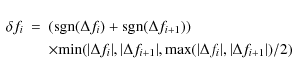
where
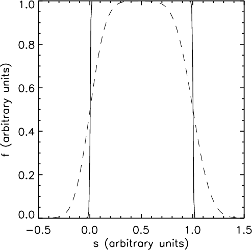 |
Figure 2: The shape of an initially rectangular pulse after convection over a distance of 4 times its width, both for the superbee scheme (solid line) and the upwind scheme (dashed line). |
| Open with DEXTER | |
Figure 2 demonstrates the effect of numerical diffusion and its mitigation in a simple 1D-model. An initially rectangular pulse has been transported by 4 length units. The simple upwind scheme has rounded the corners significantly. It can easily be seen that an ``arrival time'' based on the value of the pulse exceeding e.g. 0.1 would be strongly affected by the diffusion. The more advanced scheme, on the other hand, yields much better results, and deviations from the initial rectangular shape are hardly visible.
3.2 Test run without whistler waves
In the previous sub-section it was shown that numerical artifacts might influence the calculated electron arrival times at 1 AU. Thus, it is reasonable to test the numerical model in a simulation run without any whistler waves first. The Boltzmann-Vlasov Eq. (1) now only has the Coulomb collision term on the right hand side. But electrons with energies of several tens of keV are basically scatter-free. So we expect free propagation of flare electrons, and arrival times that can be calculated as path lengths along the Parker spiral divided by electron speed.
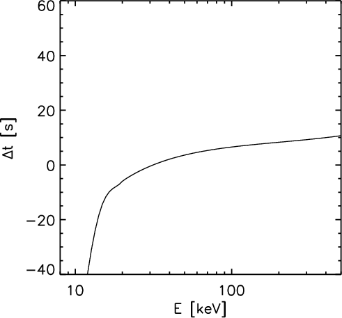 |
Figure 3:
Difference between the electron arrival times at
|
| Open with DEXTER | |
Figure 3 shows the difference ![]() between the
energetic electron arrival times calculated by the kinetic model and the
free-propagation times. These values have been obtained at a spatial position
of
between the
energetic electron arrival times calculated by the kinetic model and the
free-propagation times. These values have been obtained at a spatial position
of
![]() along the Parker spiral, that corresponds to a
radial distance of
along the Parker spiral, that corresponds to a
radial distance of
![]() from the Sun.
from the Sun.
A positive ![]() means that the energetic electrons in the kinetic model
arrive later than expected from free propagation. The figure shows that there
is a delay of 10 s for the highest electron energies of about 500 keV. The
delay decreases with decreasing energy, and becomes negative for energies
below 30 keV.
means that the energetic electrons in the kinetic model
arrive later than expected from free propagation. The figure shows that there
is a delay of 10 s for the highest electron energies of about 500 keV. The
delay decreases with decreasing energy, and becomes negative for energies
below 30 keV.
Electrons with a kinetic energy of 500 keV have speeds of
v = 0.86 c. Their
travel time over a distance of
![]() is 618 s. So an
artificial delay of 10 s in the model corresponds to an error of 1.6% in
travel time, which is fairly good. So the model has passed this
free-propagation test.
is 618 s. So an
artificial delay of 10 s in the model corresponds to an error of 1.6% in
travel time, which is fairly good. So the model has passed this
free-propagation test.
The negative values of ![]() ,
i.e. early arrival of the flare electrons,
for energies below 20 keV, are due to Coulomb collisions. The mechanism by
which scattering of electrons in momentum or energy can lead to an early
arrival of flare electrons is discussed below.
,
i.e. early arrival of the flare electrons,
for energies below 20 keV, are due to Coulomb collisions. The mechanism by
which scattering of electrons in momentum or energy can lead to an early
arrival of flare electrons is discussed below.
3.3 Pure pitch-angle diffusion
After the numerical model has shown that it yields reliable flare electron arrival times at a solar distance of about 1 AU, the effect of electron diffusion by resonant interaction with whistler waves is added. It has been shown in Sect. 2.1 that the whistler waves mainly lead to pitch-angle diffusion of the electrons under typical solar wind conditions.
Under the model assumption of pure pitch-angle diffusion, only the term
![]() needs to be considered in the quasilinear diffusion
Eq. (2). This simplification saves much computational
effort, so it is worth investigating whether it is applicable without altering
the simulation results.
needs to be considered in the quasilinear diffusion
Eq. (2). This simplification saves much computational
effort, so it is worth investigating whether it is applicable without altering
the simulation results.
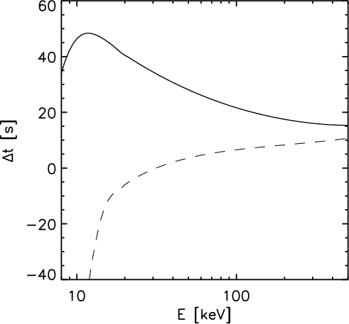 |
Figure 4:
Difference between the electron arrival times at
|
| Open with DEXTER | |
Figure 4 shows the differences between the electron
arrival times at
![]() (
(
![]() )
and the
expected times based on free propagation. The results of the simulation run
without whistler waves are also plotted for comparison.
)
and the
expected times based on free propagation. The results of the simulation run
without whistler waves are also plotted for comparison.
The results show that the pitch-angle diffusion delays the flare electrons
considerably. For high electron energies of 500 keV, the delay is only 5 s,
but it increases with decreasing energy. It is about 15 s for 100 keV, and
35 s for 30 keV. For energies little above 10 keV, the pitch-angle diffusion
counters the early arrival of flare electrons caused by Coulomb collisions,
leading to a delay of 60 s as compared to the whistler-free run, and to a peak
of ![]() in the plot.
in the plot.
So the simulation run including pitch-angle diffusion by resonant interaction with whistler waves demonstrates that the whistlers can delay electron arrival times. The maximum delay found here is of the order of 1 min.
The energy dependence of the delay also needs some attention. The
calculation of electron release times in analyses like that of Krucker
et al. (2007) is based on scatter-free electron propagation
along the path length s.

The velocity dispersion
The energy dependence of ![]() as shown in
Fig. 4 alters the
velocity dispersion
as shown in
Fig. 4 alters the
velocity dispersion
![]() and thus introduces an error into the calculation of s.
This
contribution can be estimated to be of the order of 0.02 AU for electrons with
an energy of 90 keV, leading to an error of 20 s in the release time.
and thus introduces an error into the calculation of s.
This
contribution can be estimated to be of the order of 0.02 AU for electrons with
an energy of 90 keV, leading to an error of 20 s in the release time.
![\begin{figure}
\par\includegraphics[width=12cm,clip]{11738fg5.eps}
\end{figure}](/articles/aa/full_html/2009/28/aa11738-09/img79.png) |
Figure 5:
Electron VDFs at
|
| Open with DEXTER | |
So far, only model results for the arrival times of energetic electrons at
1 AU have been presented, but not interplanetary electron VDFs during flare
electron arrival. Figure 5 shows the VDF at
![]() for four different simulation times, t.
for four different simulation times, t.
![]() corresponds to the initial
corresponds to the initial
![]() distribution. At
distribution. At
![]() the flare electrons have arrived for electron momentum
the flare electrons have arrived for electron momentum
![]() .
The pitch-angle scattering of them can be seen clearly. At
.
The pitch-angle scattering of them can be seen clearly. At
![]() ,
the energetic electrons can be found for
,
the energetic electrons can be found for
![]() .
At
.
At
![]() the flare is over, but the model heliosphere is
still filled with an isotropic halo of energetic electrons. The pitch-angle
scattering suppresses their escape through the upper boundary of the
simulation box.
the flare is over, but the model heliosphere is
still filled with an isotropic halo of energetic electrons. The pitch-angle
scattering suppresses their escape through the upper boundary of the
simulation box.
These results are based on the model assumption of pure pitch-angle
scattering. This scattering generally inhibits the transport of electrons
straight along the background magnetic field, and thus leads to delayed
arrival times at 1 AU. Diffusion along the momentum coordinate, p, has been
deemed as negligible, since the coefficient
![]() is small. However,
the plots in Fig. 5, which show the arrival of flare electrons,
indicate strong phase-space gradients along p.
is small. However,
the plots in Fig. 5, which show the arrival of flare electrons,
indicate strong phase-space gradients along p.
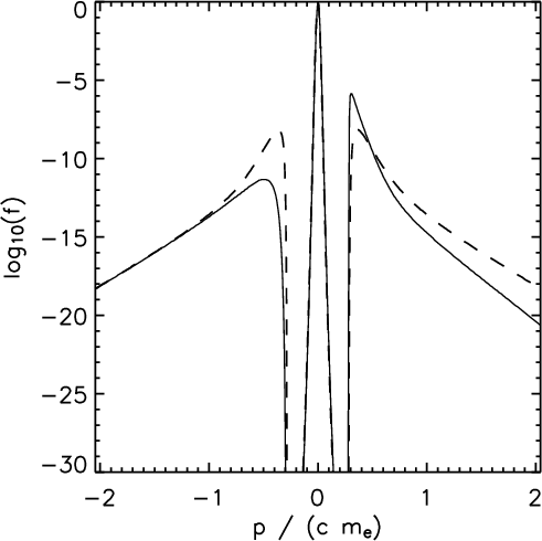 |
Figure 6:
Cuts through the electron VDF at
|
| Open with DEXTER | |
Figure 6 shows cuts through the electron VDF at
![]() during the arrival of flare
electrons at a simulation time of
during the arrival of flare
electrons at a simulation time of
![]() .
It can be seen that
the phase-space density jumps by more than 25 orders of magnitude over a
momentum interval of
.
It can be seen that
the phase-space density jumps by more than 25 orders of magnitude over a
momentum interval of
![]() .
Since a small diffusion
coefficient, multiplied by an extreme gradient, can still yield substantial
diffusion, it is now questionable whether pure pitch-angle diffusion is
appropriate for energetic electrons in interplanetary space.
.
Since a small diffusion
coefficient, multiplied by an extreme gradient, can still yield substantial
diffusion, it is now questionable whether pure pitch-angle diffusion is
appropriate for energetic electrons in interplanetary space.
Diffusion of the strong gradient in Fig. 6 would transport
electrons to lower momentum, i.e. to lower energy. Thus, at this lower energy,
the phase-space density increases earlier than expected from scatter-free
propagation, and these electrons also move further up in the box. As a
consequence, diffusion in the momentum coordinate leads to an early arrival of
energetic electrons as compared to the scatter-free expectation. This is also
the reason why non-negligible Coulomb collisions lead to negative ![]() for energies below 20 keV in the test run without whistler waves, see
Fig. 3.
for energies below 20 keV in the test run without whistler waves, see
Fig. 3.
The effect of diffusion in momentum space on the electron arrival times can be
estimated as follows. A simple diffusion equation
broadens a Gaussian distribution

Thus, the width of the phase-space gradient in Fig. 6 would also be broadened if there were no propagation effects. Replacing
For 60 keV electrons, this yields an early arrival of 10 s in our model
heliosphere. Thus, the early arrival of flare electrons due to diffusion in
momentum space is of the same order of magnitude as the delay due to
pitch-angle scattering. In other words, pure pitch-angle diffusion is not a
valid approach, although the original diffusion Eq. (2)
seems to be dominated by the pitch-angle term,
![]() .
.
3.4 Full diffusion equation
The main finding of the previous sub-section was that for solar energetic electron arrival times at 1 AU, the effect of electron diffusion along the momentum coordinate is not negligible compared to the effect of pitch-angle diffusion. So the simplification of pure pitch-angle diffusion is not allowed. The full diffusion Eq. (2) has to be implemented instead.
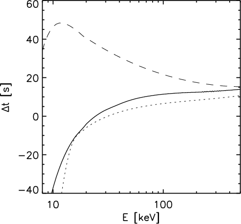 |
Figure 7:
Difference between the electron arrival times at
|
| Open with DEXTER | |
Figure 7 shows the resulting arrival times for the full
diffusion model, and the previous results for comparison. The strong delay
that has been found in the pure pitch-angle diffusion model has almost
disappeared. There is only a small difference of about ![]() compared to the free-propagation model.
compared to the free-propagation model.
This result confirms the above estimate of the influence of diffusion along the momentum coordinate on the arrival times. The early arrival of flare electrons is comparable to the delay due to pitch-angle diffusion. Thus, both parts of the full diffusion equation are capable of partly compensating each other.
It is also noteworthy that the new result for the delay of energetic electrons due to scattering in interplanetary space shows little energy dependence. The delay is rather constant, about 10 s over a wide energy range. Thus, it has little additional impact on inferred path lengths and release times of flare electrons.
3.5 Variation of the whistler wave power
All simulation results presented so far have been obtained with the whistler wave spectrum of Vocks et al. (2005) that attributes 1% of the total wave power measured in interplanetary space to the whistlers. This choice is somewhat arbitrary, and the wave spectrum might also vary in time. Thus, the effect of a variation of the wave power on the resulting electron delays needs to be investigated. This can be done by multiplying the wave spectrum by a given factor and re-running the full diffusion model.
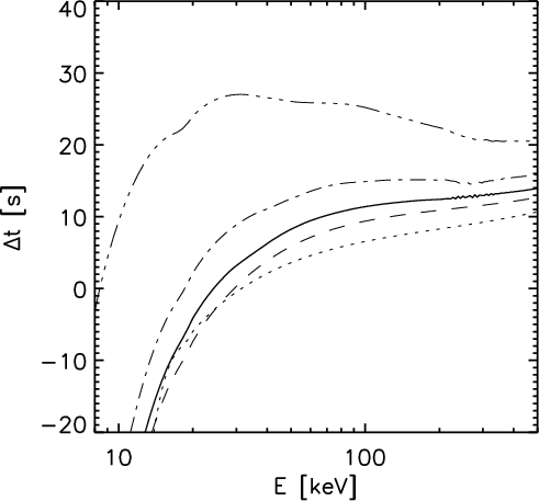 |
Figure 8:
Difference between the electron arrival times at
|
| Open with DEXTER | |
Figure 8 shows the resulting electron delays at 1 AU for five different wave spectra, ranging from no wave power up to the five-fold power as compared to the results from Fig. 7. It is evident that the delays increase with increasing wave power, as one would expect for more efficient diffusion.
The energy dependence of the delays changes slightly. For low wave powers up
to a two-fold increase, ![]() increases with increasing electron energy,
but for the highest wave power this relation is reversed. So the degree to
which the effects of pitch-angle diffusion and diffusion in the momentum
coordinate compensate each other is not independent of energy. But even for
the highest wave power, no strong energy dependence of
increases with increasing electron energy,
but for the highest wave power this relation is reversed. So the degree to
which the effects of pitch-angle diffusion and diffusion in the momentum
coordinate compensate each other is not independent of energy. But even for
the highest wave power, no strong energy dependence of ![]() is found.
is found.
The maximum delay found in this parametric study is less than 30 s, even for the highest wave intensity, and stays below 15 s for all other simulation runs.
4 Conclusions and summary
In this paper, the impact of scattering of solar energetic electrons due to resonant interaction with whistler waves in interplanetary space has been investigated. Since the quasi-linear diffusion equation seems to be dominated by the pitch-angle diffusion term, it seemed to be reasonable to simplify the model accordingly.Pitch-angle scattering leads to a delay of electron arrival times as compared to the theoretical free-propagation time from the Sun up to 1 AU. The maximum delay found in this simulation is about 1 min. This is much less than the delays of between 10 min and 30 min that are reported in the literature. So this result already indicates that pitch-angle diffusion cannot explain delays of tens of minutes.
The simulated delay shows a strong energy dependence that is strongest for low energies of about 20 keV. This energy dependence can influence the derivation of release times and path lengths of the electrons. The resulting errors have been estimated as 20 s, which is also well below 10 min.
However, the pure pitch-angle diffusion model turned out to be oversimplified. Since more energetic, i.e. faster electrons arrive earlier at a given solar distance, interplanetary electron VDFs develop strong phase-space gradients. This leads to significant diffusion along the momentum coordinate, i.e. in energy, despite the low diffusion coefficient in the quasilinear equation. If more energetic electrons are scattered to lower energies in interplanetary space, this leads to an earlier increase of the spectral flux at this lower energy at any position further away from the Sun, e.g. at 1 AU.
So diffusion in the momentum coordinate leads to earlier electron arrival times compared to pure pitch-angle diffusion. This effect becomes clearly visible at energies of less than 20 keV. In this energy range, Coulomb collisions are not entirely negligible, although even keV solar wind electrons are still collision-free with mean free paths of the order of thousands of AU. The effects of Coulomb diffusion on electrons in the energy range of a few keV is an interesting topic for future studies and is beyond the scope of this paper.
A simple estimate of the earlier electron arrival due to diffusion along the momentum coordinate shows that this effect is of the same order of magnitude as the delay due to pitch-angle scattering. Thus, it has to be concluded that the assumption of pure pitch-angle scattering without any energy diffusion is not applicable. Instead, a full diffusion model is needed. The results obtained with the new model clearly demonstrate that these two effects indeed compensate each other. The resulting electron delays hardly differ from free-propagation times.
This provides a hint as to why analyses that are based on the assumption of free propagation yield good results, although non-negligible diffusion is present in interplanetary space. The maximum difference to free-propagation times found in a series of model runs with different wave power is below 30 s, even for the strongest diffusion.
All results presented in this paper have been obtained with the same solar wind background model, and thus with the same whistler-wave phase speeds in interplanetary space. The wave speeds are always relatively small, of the order of electron thermal speeds, and the effect of the wave-particle interaction on an electron distribution is pitch-angle diffusion in the wave frame. Thus, energetic electrons will always experience strong pitch-angle scattering in the plasma frame, independent of the exact background conditions.
But this is not the case for the diffusion component along the momentum
coordinate in the plasma frame. This component directly depends on the wave
phase-speeds, that is characterized by the electron Alvén speed
![]() .
The stronger the magnetic field, and the lower the
plasma density, the higher the phase speed.
.
The stronger the magnetic field, and the lower the
plasma density, the higher the phase speed.
So the compensation between the delay to due pitch-angle diffusion and the early arrival due to momentum (or energy) diffusion depends on the solar wind conditions. But nevertheless, the pure pitch-angle diffusion model provides an upper limit on the delays of about 1 min.
The choice of the wave spectrum is somewhat arbitrary, but comparative runs with different wave intensities show that the delays do not increase beyond 30 s, even for the strongest whistler waves. So the main result of this model is that delays of 10 min and more cannot be caused by resonant interaction with whistler waves in interplanetary space, unless unrealistically high values for the whistler wave power are assumed.
Acknowledgements
This work was supported by the German Deutsche Forschungsgemeinschaft, DFG project number MA 1376/17-1.
References
- Agueda, N., Lario, D., Roelof, E. C., & Sanahuja, B. 2005, Adv. Space Res., 35, 579 [NASA ADS] [CrossRef] (In the text)
- Bieber, J. W., Matthaeus, W. H., Smith, C. W., et al. 1994, ApJ, 420, 294 [NASA ADS] [CrossRef] (In the text)
- Cane, H. V. 2003, ApJ, 598, 1403 [NASA ADS] [CrossRef] (In the text)
- Classen, H. T., Mann, G., Klassen, A., & Aurass, A. 2003, A&A, 409, 309 [NASA ADS] [CrossRef] [EDP Sciences] (In the text)
- Haggerty, D. K., & Roelof, E. C. 2002, ApJ, 579, 841 [NASA ADS] [CrossRef] (In the text)
- Holman, G. D., Sui, L., Schwartz, R. A., & Emslie, A. G. 2003, ApJ, 595, L97 [NASA ADS] [CrossRef] (In the text)
- Isenberg, P. A., Lee, M. A., & Hollweg, J. V. 2001, J. Geophys. Res., 106, 5649 [NASA ADS] [CrossRef] (In the text)
- Kennel, C. F., & Engelmann, F. 1966, Phys. Fluids, 9, 2377 [NASA ADS] [CrossRef] (In the text)
- Klassen, A., Bothmer, V., Mann, G., et al. 2002, A&A, 385, 1078 [NASA ADS] [CrossRef] [EDP Sciences] (In the text)
- Klein, K.-L., Krucker, S., Trottet, G., & Hoang, S. 2005, A&A, 431, 1047 [NASA ADS] [CrossRef] [EDP Sciences] (In the text)
- Krucker, S., Larson, D., & Lin, R. P. 1999, ApJ, 519, 864 [NASA ADS] [CrossRef] (In the text)
- Krucker, S., Kontar, E. P., Christe, S., & Lin, R. P. 2007, 663, L109, (In the text)
- Lin, R. P. 1974, Space Sci. Rev., 16, 189 [NASA ADS] [CrossRef] (In the text)
- Lin, R. P., Krucker, S., Hurford, G. J., et al. 2003, ApJ, 595, L69 [NASA ADS] [CrossRef] (In the text)
- Ljepojevic, N. N., & Burgess, A. 1990, Proc. R. Soc. Lond. A, 428, 71 [NASA ADS] [CrossRef] (In the text)
- Mangeney, A., Salem, C., Veltri, P. L., & Cecconi, B. 2001, Intermittency in the Solar Wind Turbulence and the Haar Wavelet Transform, In Sheffield Space Plasma Meeting: Multipoint Measurements versus Theory, ESA SP-492, 53 (In the text)
- Marsch, E. 1998, Nonlinear Proc. in Geophys., 5, 111 [NASA ADS] (In the text)
- Marsch, E., & Tu, C.-Y. 2001, J. Geophys. Res., 106, 227 [NASA ADS] [CrossRef] (In the text)
- Salem, C. 2000, Ph.D. Thesis, Univ. Paris (In the text)
- Thejappa, G., Goldstein, M. L., MacDowall, R. J., Papadopoulos, K., & Stone, R. G. 1999, J. Geophys. Res., 104, 28279 [NASA ADS] [CrossRef] (In the text)
- Vocks, C., Salem, C., Lin, R. P., & Mann, G. 2005, ApJ, 627, 540 [NASA ADS] [CrossRef] (In the text)
- Vocks, C., Mann, G., & Rausche, G. 2008, A&A, 480, 527 [NASA ADS] [CrossRef] [EDP Sciences] (In the text)
- Warmuth, A., Mann, G., & Aurass, H. 2009, A&A, 494, 677 [NASA ADS] [CrossRef] [EDP Sciences] (In the text)
- Yang, H. Q., & Przekwas, A. J. 1992, J. Comp. Phys., 102, 139 [NASA ADS] [CrossRef] (In the text)
All Figures
| |
Figure 1:
Cut along the line
|
| Open with DEXTER | |
| In the text | |
| |
Figure 2: The shape of an initially rectangular pulse after convection over a distance of 4 times its width, both for the superbee scheme (solid line) and the upwind scheme (dashed line). |
| Open with DEXTER | |
| In the text | |
| |
Figure 3:
Difference between the electron arrival times at
|
| Open with DEXTER | |
| In the text | |
| |
Figure 4:
Difference between the electron arrival times at
|
| Open with DEXTER | |
| In the text | |
| |
Figure 5:
Electron VDFs at
|
| Open with DEXTER | |
| In the text | |
| |
Figure 6:
Cuts through the electron VDF at
|
| Open with DEXTER | |
| In the text | |
| |
Figure 7:
Difference between the electron arrival times at
|
| Open with DEXTER | |
| In the text | |
| |
Figure 8:
Difference between the electron arrival times at
|
| Open with DEXTER | |
| In the text | |
Copyright ESO 2009
Current usage metrics show cumulative count of Article Views (full-text article views including HTML views, PDF and ePub downloads, according to the available data) and Abstracts Views on Vision4Press platform.
Data correspond to usage on the plateform after 2015. The current usage metrics is available 48-96 hours after online publication and is updated daily on week days.
Initial download of the metrics may take a while.