Distribution of jets and magnetic fields in a coronal hole

S. Kamio; H. Hara; T. Watanabe; W. Curdt

doi:10.1051/0004-6361/200811125

Free Access

Issue		A&A Volume 502, Number 1, July IV 2009


Page(s)		345 - 353
Section		The Sun
DOI		https://doi.org/10.1051/0004-6361/200811125
Published online		27 May 2009

Distribution of jets and magnetic fields in a coronal hole

S. Kamio^1,2 - H. Hara¹ - T. Watanabe¹ - W. Curdt²

1 - Hinode Science Center, National Astronomical Observatory, 2-21-1 Osawa, Mitaka 181-8588, Japan
2 - Max-Planck-Institut für Sonnensystemforschung, 37191 Katlenburg-Lindau, Germany

Received 10 October 2008 / Accepted 19 May 2009

Abstract
Context. Recent observations of ubiquitous jets in coronal holes suggest that they play an important role in coronal heating and solar wind acceleration.
Aims. The aim of our study is to understand the magnetic connectivity and the formation of jets in coronal holes. The study of jets also helps to understand the magnetic field configuration in the coronal hole.
Methods. A coordinated observation between EIS and SUMER was carried out in a polar coronal hole to investigate both the transition region and the corona. Spectropolarimeter (SP) data allowed us to examine the relationship between the distribution of jets and magnetic fields in the photosphere.
Results. Coronal jets as well as explosive events and cool upflows were identified from EIS and SUMER data. The location of these events are correlated with network fields in the photosphere.
Conclusions. Footpoints of coronal jets are connected to patches of vertical kG fields in the photosphere, which are thought to anchor open fields in the upper corona. Explosive events and cool upflows occur in network regions which harbor low-lying fields in the transition region.

Key words: Sun: corona - Sun : transition region - Sun: UV radiation

1 Introduction

Recent observations by the X-ray Telescope (XRT; Golub et al. 2007) on board Hinode (Kosugi et al. 2007) revealed the dynamic behavior of jets in polar coronal holes (Savcheva et al. 2007; Shimojo et al. 2007). Detailed analysis of XRT observations in coronal holes indicated that X-ray jets occurred with a high frequency of 60 events per day. In addition to the apparent motion seen by XRT, Kamio et al. (2007) detected Doppler shifts in coronal jets with the Extreme ultraviolet Imaging Spectrometer (EIS; Culhane et al. 2007a) on board Hinode. These results contradict earlier ideas of coronal holes being quiet. Cirtain et al. (2007) suggested that frequent occurrence of jets can partly contribute to mass transport of the fast solar wind. On top of that, the study of the energy release process of jets is important for understanding coronal heating. Shibata et al. (1992) demonstrated that jets are produced by magnetic reconnection between pre-existing fields and newly emerging fields. It is, therefore, crucial to study the connection between magnetic fields.

A combination of SUMER (Wilhelm et al. 1995) on board SOHO and EIS provide a optimum dataset which shows dynamics in the transition region and in the corona. If cool plasma is heated to form a coronal jet, the heating and acceleration process of the jet must start in the chromosphere. Pike & Harrison (1997) found accelerating velocities along a jet in He I and in O V. While they could not derive a velocity in Mg IX ( $1 \times 10^6$ K) due to low counting statistics, our new observations could extend their study to a higher temperature.

Many jet-like events have been also found in transition region emission. Explosive events (Brueckner & Bartoe 1983; Innes et al. 1997; Dere et al. 1989), typical for their strong line profile broadening, are believed to be bi-directional jets caused by magnetic reconnection. Previous works indicate that they preferentially occur at the network boundary (Madjarska & Doyle 2003; Chae et al. 2000).

The Solar Optical Telescope (SOT; Tsuneta et al. 2008b) allows us to detect small-scale magnetic flux in high latitude regions, which are crucial for studying polar coronal holes. It is widely accepted that magnetic fields play an important role in the energy release process in the corona, but a detailed study of magnetic fields and the response of the upper atmosphere has not been performed in polar coronal holes. From a comparison between the distributions of coronal jets, explosive events, and photospheric magnetic fields, you can see whether events in the corona and in the transition region arise from the same magnetic field configuration or not. This gives an insight into the connection between the photosphere and the corona, which is essential for understanding coronal heating.

The organization of the paper is as follows. The scheme of the coordinated observation is described in Sect. 2. Data reduction procedures are explained in Sect. 3, followed by results and classification of events in Sect. 4. The interpretation and discussion on the relationship between identified events and magnetic fields is presented in Sect. 5. Finally, conclusions are summarized in Sect. 6.

2 Observations

A southern polar coronal hole was observed with EIS and SUMER on April 8, 2007. It was an optimal time for observing the south pole as it was tilted towards the Earth. The aim of this coordinated observation is to study the dynamics of jets in a coronal hole over a wide temperature range.

We obtained one raster scan with EIS and SUMER to study the spatial distribution of events. The EIS scanned a 256 $^{\prime\prime}$ $\times$ 256 $^{\prime\prime}$ area with 1 $^{\prime\prime}$ step from 14:15 UTC to 17:55 UTC. Both 170 Å to 210 Å and 250 Å to 290 Å windows were recorded with 50 s exposure by EIS. Lines of Fe XII ( $\log T_{\rm e} = 6.1$ ) and He II ( $\log T_{\rm e} = 4.7$ ) are extracted from the EIS spectra for detailed analysis.

SUMER completed a 300 $^{\prime\prime}$ $\times$ 300 $^{\prime\prime}$ raster with 1.024 $^{\prime\prime}$ step from 14:01 UTC to 18:01 UTC. The emission lines in N IV $\lambda$ 765.15 ( $\log T_{\rm e}=5.2$ ), Ne VIII $\lambda$ 770.41 ( $\log T_{\rm e}=5.8$ ), S V $\lambda$ 787.47 ( $\log T_{\rm e}=5.2$ ), and O IV $\lambda$ 790.20 ( $\log T_{\rm e}=5.2$ ) were transmitted.

In this paper, the He II, O IV, Ne VIII, and Fe XII emission lines were selected for detailed analysis because they are prominent in a coronal hole and range from $\log T_{\rm e} = 4.7$ to 6.1. The radiance map in each line is presented in Fig. 1. These four emission lines clearly demonstrate the variation of solar structure with temperature.

$\begin{figure} \par\includegraphics[width=18cm,clip]{11125f1.eps} %\end{figure}$

Figure 1:

Left column: radiance in He II, O IV, Ne VIII, and Fe XII displayed in log scale. Display ranges are $2 \times 10$ - $9 \times 10^2$ erg cm^-2 s^-1 sr^-1 for He II, $2 \times 10^{-1}$ - $6 \times 10$ mW m^-2 sr^-1 for O IV, $3 \times 10^{-1}$ - $2 \times 10$ mW m^-2 sr^-1 for Ne VIII, and 4- $1 \times 10^3$ erg cm^-2 s^-1 sr^-1 for Fe XII. Right column: doppler velocities derived from He II, O IV, Ne VIII, and Fe XII. Display scales are $\pm$ 40 km s^-1. Overlaid blue and red contours indicate Stokes V (circular polarization) processed from SOT/SP data. The contour level is $\pm 2.5\times 10^{-3}$ in polarization degree. Yellow contours indicate Stokes Q (linear polarization) signal at $-1.5\times 10^{-3}$ , which outlines strong magnetic field in north-south direction. Location of events are shown with corresponding marks; Box: upflows Triangle: downflows Cross: line broadenings Circle: transient coronal jets ``X'': persistent coronal jets.

Open with DEXTER

Emission in O IV shows bright network pattern in the transition region while radiance in Fe XII indicates isolated bright points in the corona. The Ne VIII emission, which is an intermediate temperature between them, shows some of the network structure and footpoints of the coronal bright points.

Hinode XRT obtained a sequence of context images at a cadence of one minute with the Al_poly and Ti_poly filters, which are sensitive to low temperatures down to $\log T_{\rm e} = 6.0$ . Coronal images allow us to see the duration of coronal events, which complement the spectroscopic observations. They are also used to establish alignment since the XRT field of view included that of all other telescopes.

Polarization degrees in Fe I $\lambda$ 6301.5 and $\lambda$ 6302.5 were acquired by the Spectropolarimeter (SP) of SOT. They are measures of magnetic fields in the photosphere. Its 0.3 $^{\prime\prime}$ resolution allows us to study fine magnetic flux elements in network boundaries within the polar coronal hole. An area of 328 $^{\prime\prime}$ $\times$ 164 $^{\prime\prime}$ region was scanned from 13:02 UTC to 15:56 UTC. As the scanning instruments, namely EIS, SUMER, and SP, were not synchronized and their observations are not strictly simultaneous, only long lasting features can be directly compared. Nevertheless, the overall structure of the network and distribution of X-ray bright points remained unchanged during the coordinated observations. It is reasonable to compare magnetic fields in the network, jets and bright points.

3 Data reduction

3.1 Calibrations

The EIS data were reduced by using standard procedures provided in Solar Software (SSW; Freeland & Handy 1998). First, dark-current subtraction was applied to the spectra. Then spikes due to cosmic-rays and hot pixels were marked as invalid pixels.

Standard procedures from the SUMERsoft library have been applied to correct for decompression, flatfield correction, local-gain depression and deadtime correction, geometrical distortion correction, and radiometric calibration.

The SP measures polarizations in Fe I $\lambda$ 6301.5 & 6302.5. Maps of the degree of polarization were processed from the SP data by using sp_prep, a polarization calibration procedure provided in the SSW tree (Ichimoto et al. 2008). In the weak field approximation of the Zeeman effect, which is considered to be valid in quiet regions, the degree of polarization is proportional to the magnetic field strength. Since the circular polarization is sensitive to longitudinal fields, polarization degree in Stokes V is used as a measure of longitudinal fields. Similarly, linear polarizations are produced by magnetic fields perpendicular to the line-of-sight. A negative signal in Stokes Q is used as a proxy for N-S direction magnetic fields, although their polarities are not determined due to the 180 degree ambiguity of the Zeeman effect.

3.2 Alignment

In order to co-align the EIS and SUMER data, O V $\lambda$ 192.90 was retrieved from EIS to align with O IV $\lambda$ 790.20 from SUMER, which show similar network structures. Although the wing of O V $\lambda$ 192.90 is partly blended with Fe XI $\lambda$ 192.83, a clean radiance map in O V can be obtained by integrating the line core of the O V $\lambda$ 192.90. Since the network structures are in good agreement between the two data sets, the accuracy of the alignment should be comparable to the pixel size, about 1 $^{\prime\prime}$ . Fe XII and He II are recorded by two different detectors of EIS, and the spatial offset between the detectors in N-S direction has been compensated for.

XRT is employed for the alignment of EIS and SOT because it is not possible to align EIS and SOT directly. The offset between EIS and XRT was determined by using Fe XII radiance map and soft X-ray image, which have bright points and the solar limb in common. Co-alignment between SOT and XRT was carried out in accordance with Shimizu et al. (2007).

3.3 Refining He II spectra

Although He II $\lambda$ 256.32 is a powerful tool to diagnose the transition region, it suffers from coronal line blends (Young et al. 2007). Effects of coronal lines on He II spectra must be assessed to recover transition region properties. CHIANTI atomic database v5.2 (Dere et al. 1997; Landi et al. 2006) estimates that the Si X $\lambda$ 256.37 to Si X $\lambda$ 261.04 ratio is a constant value of 1.1, independent of the density of emitting plasma. The amplitude of Si X $\lambda$ 256.37 component was estimated by using Si X $\lambda$ 261.04 and was subtracted from He II spectra.

Contributions from other coronal lines, namely Fe XII $\lambda$ 256.41 and Fe XIII $\lambda$ 256.42 were estimated from Fe XII $\lambda$ 195.12 and Fe XIII $\lambda$ 202.04. Even though CHIANTI predicts these radiance ratios are density dependent and are not constant, it is still worthwhile to estimate the effect by taking the worst case values. The ratio of Fe XII $\lambda$ 256.41 / $\lambda$ 195.12 is 0.1 or lower over the density range of 10⁶-10¹⁴. Similarly, Fe XIII $\lambda$ 256.42 / $\lambda$ 202.04 is lower than 1.5. Taking the average emission of Fe XII $\lambda$ 195.12 and Fe XIII $\lambda$ 202.04. in the coronal hole, estimated emissions in Fe XII $\lambda$ 256.41 and Fe XIII $\lambda$ 256.42 contribute to about 0.1 of emission in $\lambda$ 256.32. Blends in He II have only a minor contribution in a coronal hole where coronal emissions are weak. But it must be noted that they are not negligible in coronal bright points. Enhancements in the blue-wing of the spectra, however, are attributed to He II since all blends are positioned in the red wing of He II line.

3.4 Gaussian fitting

Single Gaussian fitting was applied to EIS and SUMER data to derive radiance, Doppler shift, and full width at half maximum (FWHM). The rest wavelength must be known to determine Doppler shifts, but there is no absolute wavelength standards in the spectra. Spectra obtained with EIS shows periodic shifts in wavelength direction, which is caused by temperature variation of the instrument (Brown et al. 2007). In order to compensate for this, the average position of the spectra at each exposure was taken as a reference. The mean velocity in each spectral line was assumed to be zero by taking the average wavelength.

However, previous papers have reported that it is not true for the corona and the transition region. Sandlin et al. (1977) found a net blueshift of 6 km^-1in Fe XII spectra. Peter & Judge (1999) reported a temperature dependence of net Doppler shifts and showed that redshift at 10⁵ K could be as large as 10 km s^-1. Considering the zero velocity ambiguity, Doppler velocities greater than 10 km s^-1 were studied in this paper.

In some cases, especially in jets, spectra indicated asymmetric profiles which deviate from a Gaussian profile. For particular events shown in the next section, multiple Gaussian component fits were applied to get a better understanding of their dynamics.

4 Results

4.1 Classification of events

Significant events in velocities and line widths were identified using the following criteria. Standard deviations ( $\sigma$ ) of velocity and FWHM in each emission line were calculated. The pixels with a blueshift, redshift, or increase in line width exceeding 3 $\sigma$ levels were marked as significant events. Significant events are identified by grouping pixels with significant red, blue shifts or increased line widths. Any of the 8 surrounding pixels are grouped together. Single pixel events were ignored as they might be caused by noise. The events occupying adjacent two pixels or more were selected as significant events.

Identified events were categorized according to the velocity and line width properties. Coronal jets were defined as upflow events in the corona which were identified in velocity maps. Comparison with soft X-ray image indicates that the coronal upflow events are connected to X-ray bright points. X-ray bright points are isolated bright features in soft X-ray whose diameter is about $1{-}2 \times 10^4$ km , and they are round or loop shapes.

The coronal jets were categorized into two groups according to the durations of the associated X-ray bright points. The sequence of X-ray images allows us to trace the temporal evolution of X-ray bright points, though the temporal change of velocity could not be studied with slow raster scans by spectrometers. A coronal jet is defined as a transient coronal jet, if it is associated with a bright point that has a lifetime of less than 30 mn. A persistent coronal jet is one that is associated with a bright point that has a lifetime of more than one hour.

In the transition region line, events with significant blueshifts or redshifts are respectively classified as upflows or downflows, respectively. Here we assume that observed velocities are line-of-sight component of the upflow or downflow in the radial direction. Line broadenings without significant Doppler velocity are categorized as explosive events. Some significant upflows and downflows coincided with line broadenings. However, they are classified as upflows or downflows rather than line broadening events. Their line profiles show a superposition of a blue-shifted or red-shifted component and a stationary component, which leads to line broadenings. In the case of explosive events, both red and blue wings are enhanced and velocity changes are not significant. In the following section, multi-component fits are applied for selected events to study their properties.

Figure 1 shows the distribution of radiance, Doppler velocity, and detected events in all He II, O IV, Ne VIII, and Fe XII. The boxes, triangles, and crosses on the plot indicate locations of upflows, downflows, and line broadenings, respectively. In radiance and velocity panels in Fe XII, circles and ``X'' mark transient and persistent coronal jets in Fe XII. Overlaid red and blue contours indicate polarities of longitudinal magnetic fields obtained with Stokes V measurements. The yellow contours shows linear polarization inferred from the Stoke Q measurements, which correspond to strong magnetic fields normal to the local surface.

Cool upflows and downflows in He II and O IV are small in size, roughly $3\times 10^3$ km (4 pixels in EIS and SUMER). Most of them are not accompanied by coronal features, though there are some associated flows at the foot point of coronal jets. The line broadenings without significant net velocity are classified into explosive events. These cool events are distributed near the bright network patches in He II and O IV (Fig. 1).

The events identified in Fe XII are upflows and downflows associated with transient coronal jets. They are attached to transient bright points or stable bright points in the corona. No isolated downflow is found in the corona. Transient and stable bright points are distinguished using a series of XRT images. Transient brightening disappeared within 30 mn, while stable bright points lasted for more than one hour.

The Ne VIII in Fig. 1 shows intermediate characteristics: upflows, downflows, and line broadenings like in O IV as well as coronal jets similar to Fe XII.

4.2 Properties of events

4.2.1 Persistent jets with bright points

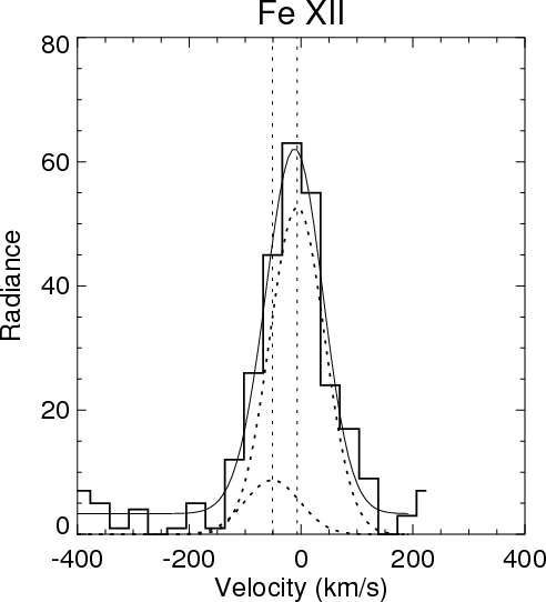$\begin{figure} \par\includegraphics{11125f2.eps} \end{figure}$	Figure 2: Fe XII spectrum from the persistent coronal jet, which is marked A in Fig. 1. Two Gaussian component fit gives velocities of -50 km s^-1 and +8 km s^-1.
Open with DEXTER

Figure 2 displays a Fe XII spectrum of the coronal jet associated with a persistent bright point which is located in the left of A in Fig. 1. In the Fe XII radiance map, a prominent bright point was seen. This bright point lasted for more than 3 h in the sequence of XRT images, thus it was classified as a persistent bright point. In the Doppler velocity map of Fe XII, a streak of blueshift of about -20 km s^-1is attached to the bright point. But the upflow event is weak in radiance and is only detectable outside the bright point.

A two Gaussian component fit to Fe XII gives a -50 km s^-1 blue-shifted component and a 8 km s^-1component (Fig. 2). Assuming that the blue-shifted and rest components respectively represent the jet and the background radiation, the line of sight component of jet velocity is -50 km s^-1.

If the jet was rooted in the position of the bright point and the flow direction was perpendicular to the local surface of the Sun, the angle between the jet and plane of the sky is estimated to be 15 degree which yields a flow velocity of about -200 km s^-1.

The eastern part of the bright point was blue-shifted by about 10 km s^-1, while the western part was red-shifted. Detected velocities inside the bright point are possibly a flow along the loop in the bright point.

In He II, no significant velocity was found at the jet or bright point. Persistent jets were only found in the coronal Fe XII line. Two persistent jets were identified in this data set. Coronal jets reported by Kamio et al. (2007) fall into this category of jets associated with persistent bright points.

4.2.2 Transient coronal jets

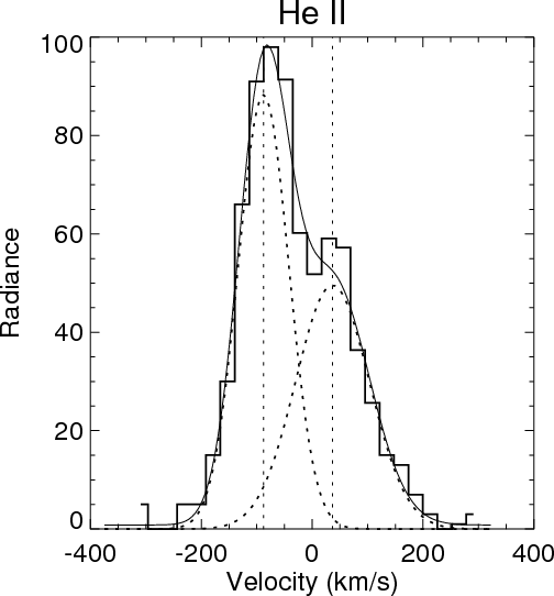$\begin{figure} \par\includegraphics{11125f3.eps} \end{figure}$	Figure 3: He II spectrum at the footpoint of the transient coronal jet, which is marked B in Fig. 1. The spectrum consists of a primary component of -88 km s^-1 and a secondary component of +37 km s^-1.
Open with DEXTER

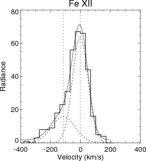$\begin{figure} \par\includegraphics{11125f4.eps} \end{figure}$	Figure 4: The Fe XII spectrum at the transient jet is composed of a -2 km s^-1 main component and a -96 km s^-1 sub component.
Open with DEXTER

Four transient coronal jets were also found in Fe XII. Figures 3 and 4 present the spectra obtained in a transient jet in He II and in Fe XII. The duration of the associated transient bright point was determined from the series of XRT images and was only 15 mn.

In the He II velocity map of Fig. 1, the blue-shifted feature in He II is confined near the footpoint marked B, while no co-spatial blueshift was found in Fe XII. In the Fe XII velocity map, a blue-shifted jet extends from the blueshifted feature in He II. The velocity signature of the Fe XII jet extended to at least $3\times 10^4$ km (40 pixels in EIS) from the footpoint. An upflow in He II ( $\log T_{\rm e} = 4.7$ ) was also observed near the bright point and was connected to the the Fe XII jet.

A two component fit to the Fe XII spectrum gives velocities of -96 km s^-1 and 2 km s^-1. The blue-shifted component has a broad tail in the spectra extending to -300 km s^-1. In the He II spectrum, the dominant component has a -96 km s^-1 blue-shift, which is comparable to the jet velocity in Fe XII. As discussed in the last section, blending of coronal lines could effect the red-wing of the spectra, hence we only discuss the blue-shifted components in He II. At the west of the footpoint, a significant downflow and brightening were found in Fe XII. It could be a counter flow to the up-flowing jet in the corona.

In another transient coronal jet, the velocity structure of the jet was captured by SUMER, which is marked C in Fig. 1. The radiance in O IV shows the jet near its footpoint while Ne VIII shows an extended part of it. For this particular event, the temperature was $\log T_{\rm e}=5.2$ in the lower part of the jet, which increased to $\log T_{\rm e}=5.8$ in the higher part.

The velocity structure in the transient jet is studied since it extended parallel to the slit in north-south direction and the velocity of the jet could be measured exactly at the same time. A two component fit to the O IV and Ne VIII spectra gives rest and upflow components in the jet. Figure 5 shows the relationship between distance from the foot point and the velocity of upflow components. The profile indicates an increasing velocity over the range of $\log T_{\rm e}=5.2$ to 5.8.

The jet flow is assumed to be guided by magnetic fields in the corona. The increase in velocity and temperature along the jet suggest that acceleration and heating took place as the plasma flowed over $2\times 10^4$ km along the magnetic field.

4.2.3 Cool upflows

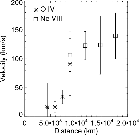$\begin{figure} \par\includegraphics{11125f5.eps} \end{figure}$	Figure 5: Doppler Velocities of upflow components in O IV and Ne VIII along the jet. The distance is measured from the jet footpoint.
Open with DEXTER

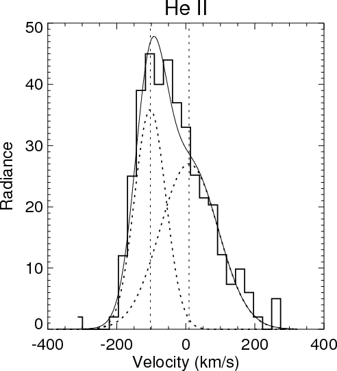$\begin{figure} \par\includegraphics{11125f6.eps} \end{figure}$	Figure 6: A blue-shifted He II spectrum obtained in the cool upflow event, which is marked D in Fig. 1. Primary and the secondary components corresponded to -93 km s^-1 and +30 km s^-1, respectively.
Open with DEXTER

Cool upflow events were found in He II and O IV emissions. They did not show any corresponding upflows in the coronal emission lines or X-rays, therefore these events were restricted below the corona. It suggests that these events were produced by an acceleration of plasma in the chromosphere which propagated into the transition region.

Figure 6 shows the He II spectrum of the largest upflow event. The upflow feature spreads over $7\times 10^3$ km (10 pixels in EIS) in the He II velocity map of Fig. 1. In the He II radiance map, a small brightening of $2\times 10^3$ km diameter was found in the north of upflow region, which is interpreted as a footpoint of the upflow event. It could be the source or trigger of the upflow event. The predominant component in He II spectrum was blue-shifted by -93 km s^-1, whose velocity is the same order of magnitude in transient coronal jets. but no significant velocity was detected in Fe XII. In O IV, 31 cool upflow events are found while only 4 events are identified in He II.

4.2.4 Cool downflows

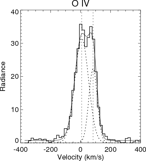$\begin{figure} \par\includegraphics{11125f7.eps} \end{figure}$	Figure 7: O IV spectrum in the cool downflow marked E in Fig. 1. A two components fit gives a +86 km s^-1 red-shifted component.
Open with DEXTER

Cool downflows without upflow signatures were also found in the transition region. Figure 7 shows the downflow event in O IV which is marked E in Fig. 1. A red-shifted component corresponding to 86 km s^-1 was found in the O IV line while no enhancement was found in the blue wing. The Ne VIII also shows a redshift in the same location. But no corresponding feature is identified in the X-ray images. In the current dataset, 2 and 19 downflow events were found in He II and O IV lines, respectively. Downflow events in He II occurred in bright network regions whose radiance is 2.5 times the spatially averaged radiance from the whole observing region. But downflow events in O IV which tend to occur on the peripheral of network regions show a 8% decrease in radiance.

4.2.5 Explosive events

Figure 8 shows an example of an explosive event spectrum found in O IV. The explosive events are characterized by line broadenings without significant velocity which is derived from single Gaussian fitting. Similar to the last two categories, the explosive events did not have coronal counterparts. Teriaca et al. (2002) has also found that the explosive events are not directly connected with the corona.

Assuming three components in the O IV spectra, both upflow and downflow components reached an amplitude of 50 km s^-1. The central component, which is assumed to be background emission, was almost at rest. Existence of the prominent rest component implies that the upflow and the downflow occupy only a small portion of the SUMER pixel. But care must be taken to compare the results with previous observations because the typical duration of explosive events is comparable to the exposure time of 50 s. Different properties might be obtained if they were observed with better temporal or spatial resolution. Nevertheless, detected line broadenings are attributed to explosive events and their locations can be compared with magnetic fields in the photosphere. In the dataset, 14 and 8 explosive events are found in He II and O IV, respectively.

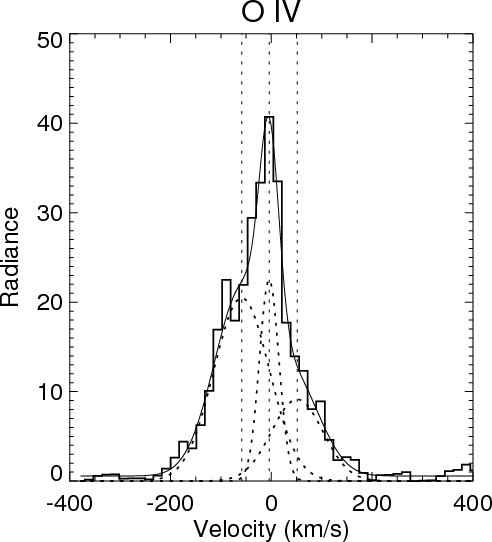$\begin{figure} \par\includegraphics{11125f8.eps} \end{figure}$	Figure 8: Broadened spectrum in O IV obtained in the explosive event. Blue-shifted and red-shifted components in O IV found to be -57 km s^-1 and +53 km s^-1, respectively.
Open with DEXTER

A remaining question is whether or not the radiance increases in explosive events. The radiance from the explosive events in He II is 30% brighter than the spatially-averaged radiance from the entire observing area. The explosive events in O IV also indicate a 10% increase in radiance. It is not clear whether the enhanced radiance is attributed to explosive events themselves, because they tend to occur in bright network regions. High cadence observations are necessary to study the radiance variations associated with explosive events. But this single scan dataset does not allow us to follow temporal changes.

5 Interpretation

$\begin{figure} \par\includegraphics[width=8cm]{11125f9.eps} \end{figure}$	Figure 9: Magnetic reconnection model of jets from Shibata et al. (1992). Magnetic reconnection occurs between newly emerging loops and open field. solid arrows presents reconnection outflows.
Open with DEXTER

Dynamic events have been identified in the EIS and SUMER data obtained in a southern polar region. Coronal jets show significant upflow velocities in Fe XII (10⁶ K). Shibata et al. (1992) proposed a model of jets in which emerging magnetic fields reconnect with pre-existing fields in the corona. Figure 9 shows the formation of a jet. Magnetic reconnection occurs between emerging closed-loop fields and open fields. In the right of Fig. 9, reconnected field forms small loops. Heating by reconnection leads to chromospheric evaporation at the footpoints of the reconnected loop. In the left of Fig. 9, the reconnected open field guides the evaporation upward to produce a hot jet, which is observed in coronal emission. Separately, the magnetic tension force of reconnected field accelerates the plasma, which produces a reconnection outflow. An MHD simulation by Yokoyama & Shibata (1995) showed that a cool jet is formed adjacent to the hot jet. Cool plasma is accelerated by magnetic force and pressure after the magnetic reconnection.

The geometry of a persistent coronal jet (Fig. 1) fits well into the schematic model in Fig. 9. The persistent bright point corresponds to the reconnected loop, and the hot jet on the other side is formed above the bright point. In order to sustain persistent bright points, heating must continue for several hours since the lifetime of the bright points are much longer than the cooling time scale of coronal loops. One of the questions is whether long-lasting reconnection occurs in bright points.

Tracking the evolution of magnetic fields is important when examining the jet model, since it requires an emerging magnetic flux to cause reconnection. Another issue is that the signature of the upflow, which is expected from the jet model, was not detected in the footpoints of the jet. The bright point and the jet are not independent events because the upflow was attached to the bright point. A possible explanation is that the emission from the bright point was dominated by the dense hot loop formed after the reconnection, and the upflow did not have detectable emission near the bright point. In the case of the transient coronal jet, the upflow component had weaker emission than the stationary component which is regarded as background emission in the coronal hole (Fig. 4).

The transient coronal jet in Fig. 1 can be explained by the jet model. An elongated jet in Fe XII corresponds to a hot jet in Fig. 9. The double component fit to the spectra gives a line of sight velocity of 96 km s^-1. Assuming a radial flow, the actual velocity reaches 300 km s^-1, which agrees with the typical velocities inferred from apparent motion in X-ray images (Shimojo et al. 2007). Although it is not so enhanced in the radiance map, the upflow in the velocity map extends to at least $3\times 10^5$ km (marked B in Fig. 1). The downflow in the west of the jet could be a counter flow to the upflowing jet, which fits well into the configuration of Fig. 9. Upflows in He II corresponds to upflows near the footpoints, which extends into the upflow in Fe XII. Alternatively, there might be a cool jet adjacent to the hot jet, which is driven by magnetic tension and pressure by reconnected fields. Canfield et al. (1996) identified a cool H $\alpha$ jet neighboring a hot X-ray jet. Since the hot jet in Fe XII and cool jet in He II were only separated by $5\times 10^3$ km, they could be neighbouring jets.

Figure 5 shows the velocity structure in the transient coronal jet (marked C in Fig. 1). The velocity profiles show upflow velocities near the foot point in O IV and the upper part in Ne VIII. According to Yokoyama & Shibata (1995), the acceleration by magnetic force only works near the footpoint of elongated jets (Fig. 9). On the contrary, acceleration by chromospheric evaporation works as long as a pressure gradient exists. Therefore, the velocity profile in Fig. 5 favors acceleration over a long distance by chromospheric evaporation. The smooth transition of velocity from O IV to Ne VIII (Fig. 5) implies that they are different temperature ranges of the same upflow. Shimojo et al. (2001) carried out a one-dimensional MHD simulation of a jet including chromospheric evaporation and found the temperature increase along the jet. The temperature increase identified from the observed jet agrees with their simulation. In addition, if velocities of Fig. 5 are projected into the radial direction, the maximum velocity corresponds to 350 km s^-1, which is comparable to their estimation. The maximum velocity of the evaporation flow is $3 \times C_{\rm S}$ where $C_{\rm S}$ is the local sound speed (Shibata et al. 1992). The sound speed is 120 km s^-1 at $6\times10^5$ K, hence the detected upflow can be explained as the evaporation flow. Chifor et al. (2008) found that there was a correlation between the density increase inside a jet in an active region and the upflow velocity, suggesting chromospheric evaporation in the jet. But it must be noted that magnetic forces can also be responsible for the supersonic jet. The jet velocity due to the unwinding magnetic flux can reach $2\times V_{\rm A}$ where $V_{\rm A}$ is the local Alfvén velocity (Shibata et al. 1992). Cirtain et al. (2007) reported the apparent velocity of jets reaches 800 km s^-1 which is close to the Alfvén speed in the corona.

Apart from coronal jets, cool upflows were found in the transition region. Although Canfield et al. (1996) showed that coronal jets are accompanied by cool jets, the cool upflows in this dataset did not show a coronal counterpart. They should result from the acceleration of cool plasma. Yokoyama & Shibata (1996,1995) demonstrated that a cool jet is generated as well as hot jet due to magnetic tension and pressure from reconnected field (Fig. 9). Cool upflows in Sect. 4.3 can be explained as cool jets. But the heating must be small so that a hot jet is not detected in coronal temperatures. These characteristics of cool upflows are similar to H $\alpha$ surges and macro spicules on the limb (Wilhelm 2000). Shibata et al. (2007) found Anemone jets in Ca II H and claimed that they are generated by small reconnections throughout the chromosphere. Ubiquitous reconnections can also occur in the transition region to produce cool upflows.

A possible explanation for cool downflows is the cooling of coronal plasma. It is not a counterflow of the up-flowing jet because of the absence of coronal emission. Culhane et al. (2007b) analyzed the evolution of jets and found that radiance enhancements in hot coronal lines were followed by enhancements in transition region lines. They concluded that the post-jet enhancement in the cool line was caused by the falling back of plasma ejected by the jet. Cool downflows in the transition region might be the aftermath of coronal jets.

Explosive events are believed to be generated by magnetic reconnection in the transition region. Figure 1 presents a comparison of the magnetic field distribution and the locations of coronal jets, cool upflows, downflows, and explosive events. Their frequent occurrence near bright network structure implies their interaction with network fields (Madjarska & Doyle 2003; Chae et al. 2000). Contours of Stokes Q are overlaid on Stokes V which originated from the LOS component of network fields. The negative signal in Stokes Q indicate perpendicular fields in the north-south direction. Tsuneta et al. (2008a) performed an inversion of the Stokes profiles obtained with SOT/SP and showed that patches of strong Stokes Q signal corresponded to kG fields in polar regions. Although the polarity of the perpendicular field can not be determined from linear polarization due to an azimuth ambiguity of the Zeeman effect, the polarities are determined from LOS component polarities inferred from Stokes V. The polarities of Stokes Q patches agrees with the dominant polarity of the polar coronal hole, which is consistent with Tsuneta et al. (2008a).

$\begin{figure} \par\includegraphics[width=8cm]{11125f10.eps} \end{figure}$	Figure 10: A schematic picture showing the magnetic field configuration in a coronal hole. On the left, reconnection with kG open field forms a coronal jet. On the right, reconnection in low-lying fields causes cool jets in the transition region.
Open with DEXTER

While the number of detected jets is not large enough to draw a firm conclusion, detected coronal jets occurred preferentially above kG magnetic patches in the photosphere. The kG patches are about 1 $^{\prime\prime}$ in diameter while corresponding jets seen by EIS/SUMER are roughly 1-2 $^{\prime\prime}$ in diameter, which are close to the instrumental resolution. Tsuneta et al. (2008a) suggested that magnetic fields in kG patches fan out from the photosphere into the upper corona. Open magnetic fields reaching the corona are essential for producing jets by reconnection (Fig. 9) One exception, a transient jet marked B in Fig. 1 is not connected to kG patch, possibly because the time difference between SOT/SP and EIS observations is three hours at this location. There is a possibility of the magnetic configuration changing between observations. In order to investigate the evolution, field measurements with better temporal resolution, such as magnetograms, are necessary for future observations.

These kG patches in the photosphere are considered to be the roots of open fields in a coronal hole. But only a small number of kG patches are associated with coronal jets. This is because the interaction between open fields and surrounding fields with an anti-parallel component is necessary for making impulsive reconnection. The existence of open field alone is not sufficient to produce jets. Raouafi et al. (2008) claimed that most of the coronal jets were followed by plume haze seen in the EUV. They suggested that the impulsive reconnection produced jets while gradual reconnection forms plumes by releasing the plasma trapped in formally closed loop. A more detailed study is needed to establish the relationship between plumes and magnetic fields.

Cool upflows and explosive events are correlated with network fields in Stokes V maps. But cool events are not correlated with kG patches. They are caused by reconnection analogous to coronal jets, but high speed flows are constrained in the lower atmosphere because of the low-lying configuration of the fields. The lack of coronal signatures in cool events also supports this scenario.

It is interesting to compare event distributions in different temperatures. More explosive events are detected in He II than in O IV (Fig. 1). In addition, the majority of events in O IV are upflows and downflows. It must be noted that the observing sequences of EIS and SUMER were quite similar though they were not synchronized. Thus, the difference is attributed to the nature of He II and O IV. Our speculation is that unresolved small-scale events in low temperature tend to show line-broadenings in He II while large scale events result in isolated flows in higher temperature in O IV. The trend of isolated flows also extends to the corona. But one concern is He II and O IV spectra were respectively obtained with EIS and SUMER, and their difference might effect the results.

Figure 10 illustrates a possible configuration of coronal jets and cool events. Coronal jets are created by reconnection between kG field patches and surrounding fields. Low-lying field leads to reconnections in the transition region which results in cool upflows or explosive events. The lack of a coronal counterpart is due to a closed field configuration in the transition region. Another possibility is that the higher density in the transition region does not allow the high speed flow to reach the corona.

Schrijver & Title (2003) proposed a multi-scale magnetic carpet model in which half of the network field connected back to internetwork fields. In their model, half of the internetwork fields reach the corona, as opposed to the classical model. It implies that internetwork fields can contribute to coronal heating via reconnection. Jendersie & Peter (2006) demonstrated that magnetic connectivity from the photosphere to the corona dramatically changed with the weak internetwork field variations. It means that strong network fields and weak internetwork fields are not independent, but are interacting. Therefore, tracing the temporal evolution of magnetic fields and the coronal response is important in future observations.

6 Conclusions

1.: Footpoints of coronal jets are correlated with vertical kG magnetic fields patches in the photosphere, which are thought to anchor open fields in the upper corona.
2.: Coronal jets are classified into persistent and transient ones. The former are associated with a stable bright point and upflows are detected only in the corona. The latter are short-lived events and upflow velocities are found both in the transition region and in the corona.
3.: The velocity structure inside a transient jet was resolved. It shows that both velocity and temperature increase along the jet, which agree with a chromospheric evaporation process.
4.: Cool upflows were found in He II and O IV. Although the detected LOS velocity of -100 km s^-1 is comparable to that of coronal jets, no counterpart is seen in the corona. A possible acceleration mechanism is magnetic force as a result of reconnection in the transition region.
5.: Cool downflows are possibly caused by cooling of coronal plasma guided by network fields.
6.: Explosive events are identified in the polar coronal hole. They are brighter than the spatially averaged radiance in the transition region lines.
7.: Explosive events and cool upflows are caused by reconnections in the transition region. They are associated with network region which harbors low-lying fields.

Acknowledgements

Authors would like to thank the referee for constructive comments. Hinode is a Japanese mission developed and launched by ISAS/JAXA, with NAOJ as domestic partner and NASA and STFC (UK) as international partners. It is operated by these agencies in co-operation with ESA and NSC (Norway). The SUMER project is financially supported byDLR, CNES, NASA, and the ESA PRODEX Programme (Swiss contribution). SUMER is part of SOHO of ESA and NASA. This work was partly carried out at the NAOJ Hinode Science Center, which is supported by the Grant-in-Aid for Creative Scientific Research ``The Basic Study of Space Weather Prediction'' from MEXT, Japan (Head Investigator: K. Shibata), generous donations from Sun Microsystems, and NAOJ internal funding.

References

Brown, C. M., Hara, H., Kamio, S., et al. 2007, PASJ, 59, 865 [NASA ADS] (In the text)
Brueckner, G. E., & Bartoe, J.-D. F. 1983, ApJ, 272, 329 [NASA ADS] [CrossRef]
Canfield, R. C., Reardon, K. P., Leka, K. D., et al. 1996, ApJ, 464, 1016 [NASA ADS] [CrossRef] (In the text)
Chae, J., Wang, H., Goode, P. R., Fludra, A., & Schühle, U. 2000, ApJ, 528, L119 [NASA ADS] [CrossRef]
Chifor, C., Young, P. R., Isobe, H., et al. 2008, A&A, 481, L57 [NASA ADS] [CrossRef] [EDP Sciences] (In the text)
Cirtain, J. W., Golub, L., Lundquist, L., et al. 2007, Science, 318, 1580 [NASA ADS] [CrossRef] (In the text)
Culhane, J. L., Harra, L. K., James, A. M., et al. 2007a, Sol. Phys., 243, 19 [NASA ADS] [CrossRef] (In the text)
Culhane, L., Harra, L. K., Baker, D., et al. 2007b, PASJ, 59, 751 [NASA ADS] (In the text)
Dere, K. P., Bartoe, J.-D. F., & Brueckner, G. E. 1989, Sol. Phys., 123, 41 [NASA ADS] [CrossRef]
Dere, K. P., Landi, E., Mason, H. E., Monsignori Fossi, B. C., & Young, P. R. 1997, A&AS, 125, 149 [NASA ADS] [CrossRef] [EDP Sciences]
Freeland, S. L., & Handy, B. N. 1998, Sol. Phys., 182, 497 [NASA ADS] [CrossRef] (In the text)
Golub, L., Deluca, E., Austin, G., et al. 2007, Sol. Phys., 243, 63 [NASA ADS] [CrossRef] (In the text)
Ichimoto, K., Lites, B., Elmore, D., et al. 2008, Sol. Phys., 249, 233 [NASA ADS] [CrossRef] (In the text)
Innes, D. E., Inhester, B., Axford, W. I., & Willhelm, K. 1997, Nature, 386, 811 [NASA ADS] [CrossRef]
Jendersie, S., & Peter, H. 2006, A&A, 460, 901 [NASA ADS] [CrossRef] [EDP Sciences] (In the text)
Kamio, S., Hara, H., Watanabe, T., et al. 2007, PASJ, 59, 757 (In the text)
Kosugi, T., Matsuzaki, K., Sakao, T., et al. 2007, Sol. Phys., 243, 3 [NASA ADS] [CrossRef] (In the text)
Landi, E., Del Zanna, G., Young, P. R., et al. 2006, ApJS, 162, 261 [NASA ADS] [CrossRef]
Madjarska, M. S., & Doyle, J. G. 2003, A&A, 403, 731 [NASA ADS] [CrossRef] [EDP Sciences]
Peter, H., & Judge, P. G. 1999, ApJ, 522, 1148 [NASA ADS] [CrossRef] (In the text)
Pike, C. D., & Harrison, R. A. 1997, Sol. Phys., 175, 457 [NASA ADS] [CrossRef] (In the text)
Raouafi, N.-E., Petrie, G. J. D., Norton, A. A., Henney, C. J., & Solanki, S. K. 2008, ApJ, 682, L137 [NASA ADS] [CrossRef] (In the text)
Sandlin, G. D., Brueckner, G. E., & Tousey, R. 1977, ApJ, 214, 898 [NASA ADS] [CrossRef] (In the text)
Savcheva, A., Cirtain, J., Deluca, E. E., et al. 2007, PASJ, 59, 771 [NASA ADS] (In the text)
Schrijver, C. J., & Title, A. M. 2003, ApJ, 597, 165 [NASA ADS] [CrossRef] (In the text)
Shibata, K., Ishido, Y., Acton, L. W., et al. 1992, PASJ, 44, L173 [NASA ADS] [CrossRef] (In the text)
Shibata, K., Nakamura, T., Matsumoto, T., et al. 2007, Science, 318, 1591 [NASA ADS] [CrossRef] (In the text)
Shimizu, T., Katsukawa, Y., Matsuzaki, K., et al. 2007, PASJ, 59, 845 (In the text)
Shimojo, M., Shibata, K., Yokoyama, T., & Hori, K. 2001, ApJ, 550, 1051 [NASA ADS] [CrossRef] (In the text)
Shimojo, M., Narukage, N., Kano, R., et al. 2007, PASJ, 59, 745 (In the text)
Teriaca, L., Madjarska, M. S., & Doyle, J. G. 2002, A&A, 392, 309 [NASA ADS] [CrossRef] [EDP Sciences] (In the text)
Tsuneta, S., Ichimoto, K., Katsukawa, Y., et al. 2008a, ApJ, 688, 1374 [NASA ADS] [CrossRef] (In the text)
Tsuneta, S., Ichimoto, K., Katsukawa, Y., et al. 2008b, Sol. Phys., 249, 167 [NASA ADS] [CrossRef] (In the text)
Wilhelm, K. 2000, A&A, 360, 351 [NASA ADS] (In the text)
Wilhelm, K., Curdt, W., Marsch, E., et al. 1995, Sol. Phys., 162, 189 [NASA ADS] [CrossRef] (In the text)
Yokoyama, T., & Shibata, K. 1995, Nature, 375, 42 [NASA ADS] [CrossRef] (In the text)
Yokoyama, T., & Shibata, K. 1996, PASJ, 48, 353 [NASA ADS]
Young, P. R., Del Zanna, G., Mason, H. E., et al. 2007, PASJ, 59, 857 [NASA ADS] (In the text)

Footnotes

... library: SUMERsoft is a software library, which constitutes the integrated experience with SUMER data analysis tools. It is available at http://www.mps.mpg.de/projects/soho/sumer/text/list_sumer_soft.htm

All Figures

$\begin{figure} \par\includegraphics[width=18cm,clip]{11125f1.eps} %\end{figure}$	Figure 1: Left column: radiance in He II, O IV, Ne VIII, and Fe XII displayed in log scale. Display ranges are $2 \times 10$ - $9 \times 10^2$ erg cm^-2 s^-1 sr^-1 for He II, $2 \times 10^{-1}$ - $6 \times 10$ mW m^-2 sr^-1 for O IV, $3 \times 10^{-1}$ - $2 \times 10$ mW m^-2 sr^-1 for Ne VIII, and 4- $1 \times 10^3$ erg cm^-2 s^-1 sr^-1 for Fe XII. Right column: doppler velocities derived from He II, O IV, Ne VIII, and Fe XII. Display scales are $\pm$ 40 km s^-1. Overlaid blue and red contours indicate Stokes V (circular polarization) processed from SOT/SP data. The contour level is $\pm 2.5\times 10^{-3}$ in polarization degree. Yellow contours indicate Stokes Q (linear polarization) signal at $-1.5\times 10^{-3}$ , which outlines strong magnetic field in north-south direction. Location of events are shown with corresponding marks; Box: upflows Triangle: downflows Cross: line broadenings Circle: transient coronal jets ``X'': persistent coronal jets.
Open with DEXTER
In the text

$\begin{figure} \par\includegraphics{11125f2.eps} \end{figure}$	Figure 2: Fe XII spectrum from the persistent coronal jet, which is marked A in Fig. 1. Two Gaussian component fit gives velocities of -50 km s^-1 and +8 km s^-1.
Open with DEXTER
In the text

$\begin{figure} \par\includegraphics{11125f3.eps} \end{figure}$	Figure 3: He II spectrum at the footpoint of the transient coronal jet, which is marked B in Fig. 1. The spectrum consists of a primary component of -88 km s^-1 and a secondary component of +37 km s^-1.
Open with DEXTER
In the text

$\begin{figure} \par\includegraphics{11125f4.eps} \end{figure}$	Figure 4: The Fe XII spectrum at the transient jet is composed of a -2 km s^-1 main component and a -96 km s^-1 sub component.
Open with DEXTER
In the text

$\begin{figure} \par\includegraphics{11125f5.eps} \end{figure}$	Figure 5: Doppler Velocities of upflow components in O IV and Ne VIII along the jet. The distance is measured from the jet footpoint.
Open with DEXTER
In the text

$\begin{figure} \par\includegraphics{11125f6.eps} \end{figure}$	Figure 6: A blue-shifted He II spectrum obtained in the cool upflow event, which is marked D in Fig. 1. Primary and the secondary components corresponded to -93 km s^-1 and +30 km s^-1, respectively.
Open with DEXTER
In the text

$\begin{figure} \par\includegraphics{11125f7.eps} \end{figure}$	Figure 7: O IV spectrum in the cool downflow marked E in Fig. 1. A two components fit gives a +86 km s^-1 red-shifted component.
Open with DEXTER
In the text

$\begin{figure} \par\includegraphics{11125f8.eps} \end{figure}$	Figure 8: Broadened spectrum in O IV obtained in the explosive event. Blue-shifted and red-shifted components in O IV found to be -57 km s^-1 and +53 km s^-1, respectively.
Open with DEXTER
In the text

$\begin{figure} \par\includegraphics[width=8cm]{11125f9.eps} \end{figure}$	Figure 9: Magnetic reconnection model of jets from Shibata et al. (1992). Magnetic reconnection occurs between newly emerging loops and open field. solid arrows presents reconnection outflows.
Open with DEXTER
In the text

$\begin{figure} \par\includegraphics[width=8cm]{11125f10.eps} \end{figure}$	Figure 10: A schematic picture showing the magnetic field configuration in a coronal hole. On the left, reconnection with kG open field forms a coronal jet. On the right, reconnection in low-lying fields causes cool jets in the transition region.
Open with DEXTER
In the text

Current usage metrics show cumulative count of Article Views (full-text article views including HTML views, PDF and ePub downloads, according to the available data) and Abstracts Views on Vision4Press platform.

Data correspond to usage on the plateform after 2015. The current usage metrics is available 48-96 hours after online publication and is updated daily on week days.

Initial download of the metrics may take a while.