| Issue |
A&A
Volume 502, Number 1, July IV 2009
|
|
|---|---|---|
| Page(s) | 303 - 314 | |
| Section | The Sun | |
| DOI | https://doi.org/10.1051/0004-6361/200811117 | |
| Published online | 29 April 2009 | |
Discriminant analysis of solar bright points and faculae![[*]](/icons/foot_motif.png)
I. Classification method and center-to-limb distribution
P. Kobel1 - J. Hirzberger1 - S. K. Solanki1,2 - A. Gandorfer1 - V. Zakharov1
1 - Max-Planck Institut für Sonnensystemforschung, Max-Planck-Straße 2, 37191 Katlenburg-Lindau, Germany
2 - School of Space Research, Kyung Hee University, Yongin, Gyeonggi, 446-701, Korea
Received 9 October 2008 / Accepted 20 March 2009
Abstract
Context. While photospheric magnetic elements appear mainly as Bright Points (BPs) at the disk center and as faculae near the limb, high-resolution images reveal the coexistence of BPs and faculae over a range of heliocentric angles. This is not explained by a ``hot wall'' effect through vertical flux tubes, and suggests that the transition from BPs to faculae needs to be quantitatively investigated.
Aims. To achieve this, we made the first recorded attempt to discriminate BPs and faculae, using a statistical classification approach based on Linear Discriminant Analysis (LDA). This paper gives a detailed description of our method, and shows its application on high-resolution images of active regions to retrieve a center-to-limb distribution of BPs and faculae.
Methods. Bright ``magnetic'' features were detected at various disk positions by a segmentation algorithm using simultaneous G-band and continuum information. By using a selected sample of those features to represent BPs and faculae, suitable photometric parameters were identified for their discrimination. We then carried out LDA to find a unique discriminant variable, defined as the linear combination of the parameters that best separates the BPs and faculae samples. By choosing an adequate threshold on that variable, the segmented features were finally classified as BPs and faculae at all the disk positions.
Results. We thus obtained a Center-to-Limb Variation (CLV) of the relative number of BPs and faculae, revealing the predominance of faculae at all disk positions except close to disk center (
![]() ).
).
Conclusions. Although the present dataset suffers from limited statistics, our results are consistent with other observations of BPs and faculae at various disk positions. The retrieved CLV indicates that at high resolution, faculae are an essential constituent of active regions all across the solar disk. We speculate that the faculae near disk center as well as the BPs away from disk center are associated with inclined fields.
Key words: Sun: photosphere - Sun: faculae, plages - Sun: magnetic fields - methods: statistical - techniques: high angular resolution - techniques: photometric
1 Introduction
When imaged at high spatial resolution, the solar photosphere reveals a myriad of tiny bright features, primarily concentrated in active regions and outlining the borders of supergranules in the quiet Sun. Near disk center, they appear mainly as ``Bright Points'' (BPs) or ``filigree'' (Dunn & Zirker 1973; Mehltretter 1974), i.e. roundish or elongated bright features located in the intergranular downflow lanes (Title et al. 1987), particularly bright when observed in Fraunhofer's G-band (Langhans et al. 2002; Berger et al. 1995; Muller & Roudier 1984). Near the limb, they resemble more side-illuminated granules called ``faculae'' or ``facular grains'' (e.g. Muller 1975), herein considered as individual small-scale elements (Hirzberger & Wiehr 2005). The close association of BPs and faculae with magnetic field indicators such as chromospheric Ca II emission suggests that they are related phenomena (Mehltretter 1974; Wilson 1981), both associated with small-scale kG flux concentrations (Stenflo 1973). These so-called ``magnetic elements'' are considered as the basic building blocks of the photospheric magnetic activity (see Schüssler 1992; Solanki 1993, for reviews), whence the importance of understanding their fundamental physics. Also, much of the interest in faculae has been justified by their major role in producing the total solar irradiance variation (Walton et al. 2003; Fligge et al. 1998; Lean & Foukal 1988; Krivova et al. 2003).
Table 1: Dataset specifications.
The peculiar appearance of BPs and faculae as well as their different distribution on the disk raises questions about their physical origin and mutual relationship. The standard model accounting for both these phenomena describes BPs and faculae as distinct radiative signatures of strongly evacuated thin flux tubes, arising from different viewing angles (``hot-wall'' model, Spruit 1976; Knölker et al. 1991; Steiner 2005; Knölker et al. 1988). This simplified picture has been verified in its salient points by recent comprehensive 3D MHD simulations (Vögler et al. 2005). A major success has been the ability to qualitatively reproduce BPs near disk center (Shelyag et al. 2004; Schüssler et al. 2003) and faculae closer to the limb (Carlsson et al. 2004; Keller et al. 2004), thereby confirming the basic hot-wall model to first order. However, images with the highest spatial resolution reveal the presence of BPs away from the disk center, and of facular elements even close to the disk center (Hirzberger & Wiehr 2005; Berger et al. 2007). Such mixtures of BPs and faculae at several heliocentric positions is not explained by the hot-wall picture considering vertical flux tubes, and seems not apparent in the simulated synthetic images (Keller et al. 2004). Further, it is not clear either whether the BPs and faculae seen at different heliocentric angles are associated with similar magnetic structures, or rather with different structures prone to selection effects (Lites et al. 2004; Solanki et al. 2006). This shows that the transition from BPs to faculae is not clearly understood, and current models aiming at reproducing BPs and faculae would benefit from a quantitative study of the distribution of these features on the disk.
To tackle these issues, a necessary step is to sort the BPs and faculae observed at various disk positions, in order to treat them separately. The approach proposed here is the first attempt in this direction, and relies on Linear Discriminant Analysis (LDA) (Fischer 1936) as a basis to ``classify'' features as BPs or faculae. Our method makes use of purely photometric information, so that it only distinguishes the features appearing as BPs or as faculae. We applied this method to high-resolution images of active regions, covering a range of heliocentric angles where the transition from BPs to faculae is expected. This allowed us to retrieve, for the first time, an estimate of the center-to-limb variation of the relative amount of both features, and thereby to quantitatively grasp how the appearance of magnetic elements varies from center to limb.
Although Discriminant Analysis has been fruitfully used in Astronomy (see the general review by Heck & Murtagh 1989), its application in the framework of solar physics thus far has been restricted to the study of the conditions triggering solar flares (the aim of ``probabilistic flare forecasting'' Leka & Barnes 2003; Barnes et al. 2007; Smith et al. 1996), and to the response at the Earth's surface to the solar cycle (Tung & Camp 2008). Therefore, this paper is intended to give a detailed description of our classification method, and by the same token provides a concrete example of linear discriminant analysis applied to solar data. Among other potential applications in solar physics, we mention the taxonomy of flares and the separation of chromospheric BPs and cosmic ray spikes on wavelet-analyzed images (Antoine et al. 2002).
The structure of this paper reflects the path taken to resolve the classification problem. Section 2 describes the original dataset processing, and the automated segmentation method by which bright features were detected at each disk position. Section 3 outlines the classification scheme while briefly presenting the principles of LDA. It also gives a detailed report of how this technique can be applied to a selected sample of BPs and faculae in order to derive a single discriminant variable, based on which a simple classification rule can be built. Section 4 then deals with the actual classification of all the segmented features, as well as the discussion of these results from a methodological and physical point of view. Finally, Sect. 5 summarizes the obtained results and gives future directions for such work.
![\begin{figure}
\par\includegraphics[width=13cm,clip]{1117fig1.eps}
\end{figure}](/articles/aa/full_html/2009/28/aa11117-08/img47.png) |
Figure 1:
G-band image of NOAA 0669 at
|
| Open with DEXTER | |
![\begin{figure}
\par\includegraphics[width=13cm,clip]{1117fig2.eps}
\end{figure}](/articles/aa/full_html/2009/28/aa11117-08/img49.png) |
Figure 2:
G-band image of NOAA 0671
|
| Open with DEXTER | |
2 Image processing and segmentation
2.1 Dataset processing
The original dataset consists of simultaneous G-band (
![]() nm) and nearby continuum (
nm) and nearby continuum (
![]() nm) images recorded at the 1m Swedish Solar Telescope (SST, La Palma), on 7th and 8th September 2004. They cover
active regions at seven disk positions in the range
nm) images recorded at the 1m Swedish Solar Telescope (SST, La Palma), on 7th and 8th September 2004. They cover
active regions at seven disk positions in the range
![]() ,
where
,
where
![]() cos
cos![]() ,
,
![]() is the heliocentric angle and
is the heliocentric angle and
![]() corresponds to the center of the respective field of view (FOV), equivalent to the mean
corresponds to the center of the respective field of view (FOV), equivalent to the mean ![]() over the whole FOV (cf. Table 1). This range of disk positions contains both BPs and faculae, and is thus well-suited to investigate their
transition. Because our study requires the highest spatial resolution in order to resolve individual BPs and
faculae, the dataset was restricted to the one to three best image pairs at each disk position (obtained
at peaks of seeing), which were kept for further processing and analysis (see Table 1).
over the whole FOV (cf. Table 1). This range of disk positions contains both BPs and faculae, and is thus well-suited to investigate their
transition. Because our study requires the highest spatial resolution in order to resolve individual BPs and
faculae, the dataset was restricted to the one to three best image pairs at each disk position (obtained
at peaks of seeing), which were kept for further processing and analysis (see Table 1).
For the selected image pairs, phase-diversity reconstruction allowed a roughly constant angular resolution to be achieved, close to the diffraction limit (![]()
![]() at 430 nm). The reconstructed
simultaneous image pairs (G-band and continuum) were aligned and destretched using cross-correlation and grid warping techniques (courtesy Sütterlin). The direction of the closest limb was found by comparison with roughly co-temporal SOHO/MDI full disk continuum images, and the images were divided by the limb darkening
at 430 nm). The reconstructed
simultaneous image pairs (G-band and continuum) were aligned and destretched using cross-correlation and grid warping techniques (courtesy Sütterlin). The direction of the closest limb was found by comparison with roughly co-temporal SOHO/MDI full disk continuum images, and the images were divided by the limb darkening
![]() -polynomial of Neckel & Labs (1994) at the nearest tabulated wavelength (427.9 nm). For each image pair, the
contrast C was then defined relative to the mean intensity
-polynomial of Neckel & Labs (1994) at the nearest tabulated wavelength (427.9 nm). For each image pair, the
contrast C was then defined relative to the mean intensity
![]() of a quasi-quiet Sun subfield (of area ranging from 44 to 114 arcsec2, depending on the image) as
of a quasi-quiet Sun subfield (of area ranging from 44 to 114 arcsec2, depending on the image) as
![]() .
The G-band and continuum contrast are hereafter denoted
.
The G-band and continuum contrast are hereafter denoted ![]() and
and ![]() ,
respectively. To enhance the segmentation process (see Sect. 2.2), we applied a high-pass
spatial frequency filter to remove medium and large-scale fluctuations of the intensity (with observed spatial scales between 5 and 30
,
respectively. To enhance the segmentation process (see Sect. 2.2), we applied a high-pass
spatial frequency filter to remove medium and large-scale fluctuations of the intensity (with observed spatial scales between 5 and 30
![]() ), presumably attributable to p-modes,
supergranular cell contrasts, straylight and residual flat-field effects. The Fourier filter was of the form
), presumably attributable to p-modes,
supergranular cell contrasts, straylight and residual flat-field effects. The Fourier filter was of the form
![]() ,
where k is the modulus of the spatial frequency, and the parameter a was set to have a cut-off frequency (
F(k) = 0.5) of 0.2 arcsec-1 and full power (F(k) = 1) at 0.65 arcsec-1 (in accordance with Hirzberger & Wiehr 2005). Finally, sunspots and large pores featuring umbral dots were masked out,
together with their immediate surrounding granules. This prevents the contamination of BPs/faculae statistics by features of a different physical nature. Figures 1 and 2 show examples of G-band images at
,
where k is the modulus of the spatial frequency, and the parameter a was set to have a cut-off frequency (
F(k) = 0.5) of 0.2 arcsec-1 and full power (F(k) = 1) at 0.65 arcsec-1 (in accordance with Hirzberger & Wiehr 2005). Finally, sunspots and large pores featuring umbral dots were masked out,
together with their immediate surrounding granules. This prevents the contamination of BPs/faculae statistics by features of a different physical nature. Figures 1 and 2 show examples of G-band images at
![]() and
and
![]() ,
respectively, in which the quiet Sun contrast reference and the masked out sunspot and pore areas are outlined.
,
respectively, in which the quiet Sun contrast reference and the masked out sunspot and pore areas are outlined.
2.2 Magnetic brightening segmentation
Prior to their classification as BPs or faculae, bright magnetic features at the different disk positions of our dataset were detected by a segmentation algorithm. The aims of our algorithm were twofold:
- 1.
- Detect magnetic brightenings photometrically by comparison of their contrast in G-band and continuum.
- 2.
- Decompose groups of BPs and striated faculae into individual elements by using Multi-Level-Tracking (MLT, Bovelet & Wiehr 2001,2007,2003).
The principle behind point 1 is best illustrated by ![]() vs.
vs. ![]() scatterplots of
a plage area, as shown in Fig. 3 (see Figs. 1 and 2 for the location
of the chosen plage subfields). As can be seen in Fig. 3, the scatterplot splits into two clearly distinct pixel distributions. A similar pattern appears in the diagnostics of radiative MHD simulations of Shelyag et al. (2004), where the upper distribution is shown to be associated with strong flux concentrations, whereas the lower one corresponds to weakly magnetized granules (see also Sánchez Almeida et al. 2001, for the comparison of different 1D LTE atmospheres). We can thus select pixels which are G-band bright and likely to be of magnetic
origin by imposing two thresholds: a G-band threshold
scatterplots of
a plage area, as shown in Fig. 3 (see Figs. 1 and 2 for the location
of the chosen plage subfields). As can be seen in Fig. 3, the scatterplot splits into two clearly distinct pixel distributions. A similar pattern appears in the diagnostics of radiative MHD simulations of Shelyag et al. (2004), where the upper distribution is shown to be associated with strong flux concentrations, whereas the lower one corresponds to weakly magnetized granules (see also Sánchez Almeida et al. 2001, for the comparison of different 1D LTE atmospheres). We can thus select pixels which are G-band bright and likely to be of magnetic
origin by imposing two thresholds: a G-band threshold
![]() selecting the bright portion of the diagram (dashed lines in Fig. 3), and a threshold
selecting the bright portion of the diagram (dashed lines in Fig. 3), and a threshold
![]() on the contrast difference
on the contrast difference
![]() (see Berger et al. 1998, for more details).
(see Berger et al. 1998, for more details).
To achieve point 2, we chose a set of closely-spaced MLT levels between
![]() and
and
![]() .
The interlevel spacing was tuned to 0.02 (similar to Bovelet & Wiehr 2007, for BPs at disk center) by visual
comparison of the segmentation maps with the original images. This spacing allowed chains of BPs and faculae striations to be resolved, while avoiding over-segmentation. The structures were then extended down to
.
The interlevel spacing was tuned to 0.02 (similar to Bovelet & Wiehr 2007, for BPs at disk center) by visual
comparison of the segmentation maps with the original images. This spacing allowed chains of BPs and faculae striations to be resolved, while avoiding over-segmentation. The structures were then extended down to
![]() with two intermediate levels at
with two intermediate levels at
![]() and
and
![]() .
This extension increases the
segmented area of faculae compared to BPs, allowing its further use as discriminant parameter (see Sect. 3.3). The intermediate levels prevent the merging of BPs with adjacent granules and the clumping of granular fragments when the contrast of intergranular lanes does not drop below
.
This extension increases the
segmented area of faculae compared to BPs, allowing its further use as discriminant parameter (see Sect. 3.3). The intermediate levels prevent the merging of BPs with adjacent granules and the clumping of granular fragments when the contrast of intergranular lanes does not drop below
![]() .
Since a
necessary condition for a feature to be selected is to have its contrast maximum above
.
Since a
necessary condition for a feature to be selected is to have its contrast maximum above
![]() ,
no other
levels were included between
,
no other
levels were included between
![]() and
and
![]() to avoid oversegmentation. Likewise, structures
of less than 5 pixels in area (corresponding to the area of a roundish feature with a diameter of
to avoid oversegmentation. Likewise, structures
of less than 5 pixels in area (corresponding to the area of a roundish feature with a diameter of
![]() ,
i.e. roughly equal to the diffraction limit) were removed at each MLT level.
,
i.e. roughly equal to the diffraction limit) were removed at each MLT level.
The segmentation algorithm then proceeded in two steps: First, MLT was applied to the spatially-filtered G-band images. In a second step, structures corresponding to ``magnetic'' features were selected by requiring them to contain a minimum of 5 pixels satisfying
![]() and
and
![]() .
A binary map of segmented features was ultimately obtained for each G-band/continuum image pair.
.
A binary map of segmented features was ultimately obtained for each G-band/continuum image pair.
![\begin{figure}
\par\includegraphics[width=13.2cm]{1117fig3.eps}
\end{figure}](/articles/aa/full_html/2009/28/aa11117-08/img69.png) |
Figure 3:
|
| Open with DEXTER | |
![\begin{figure}
\par\includegraphics[width=7cm]{1117fig4.eps}
\end{figure}](/articles/aa/full_html/2009/28/aa11117-08/img70.png) |
Figure 4:
Maximum G-band contrast values (small crosses) of all features segmented only with a difference threshold
|
| Open with DEXTER | |
Unlike the G-band threshold, the difference threshold
![]() can be set to a unique value for all disk
positions, inasmuch as the ``non-magnetic'' distribution has a slope roughly equal to unity at all
can be set to a unique value for all disk
positions, inasmuch as the ``non-magnetic'' distribution has a slope roughly equal to unity at all
![]() .
To set
.
To set
![]() properly, we made use of ``test'' data consisting of a single
G-band/continuum image pair obtained with the same setup as our original dataset (and processed as in
Sect. 2.1, except for speckle reconstruction), but supplemented with SOUP (Lockheed Solar Optical Universal Polarimeter) Stokes V and I maps, recorded in the wing of the Fe I 6302.5 Å line with a detuning of 75 mÅ. Given the value of the G-band threshold for that disk position, the difference
threshold was tuned such as to minimize the fraction of ``false'' detections. By considering false detections as
having less than 5 pixels with
properly, we made use of ``test'' data consisting of a single
G-band/continuum image pair obtained with the same setup as our original dataset (and processed as in
Sect. 2.1, except for speckle reconstruction), but supplemented with SOUP (Lockheed Solar Optical Universal Polarimeter) Stokes V and I maps, recorded in the wing of the Fe I 6302.5 Å line with a detuning of 75 mÅ. Given the value of the G-band threshold for that disk position, the difference
threshold was tuned such as to minimize the fraction of ``false'' detections. By considering false detections as
having less than 5 pixels with
![]() (well above the noise level
(well above the noise level ![]() 10-2), the optimal difference threshold was found as
10-2), the optimal difference threshold was found as
![]() .
The corresponding fraction of false detections amounts to roughly 2%. These test images were, however, not used further because they were focused on a large sunspot
and hence contain a very small effective field of view (see Table 1, 13-Aug-2006).
.
The corresponding fraction of false detections amounts to roughly 2%. These test images were, however, not used further because they were focused on a large sunspot
and hence contain a very small effective field of view (see Table 1, 13-Aug-2006).
Without information about the magnetic field itself, our segmentation has to rely on purely photometric thresholds, and hence cannot detect all the magnetic features. The combined thresholds only aim at detecting a sample of bright features that is least biased by non-magnetic ones. However, the use of thresholds always implies the drawback of selection effects. In particular, the G-band threshold will neglect fainter features, especially low-contrast BPs near disk center (see Bovelet & Wiehr 2007; Title & Berger 1996; Shelyag et al. 2004).
3 Discriminant analysis of bright points and faculae
3.1 General scheme and training set
To develop an algorithmic classification method for BPs and faculae, we adopted the following scheme, that uses Linear Discriminant Analysis (LDA, a statistical technique first introduced by Fischer 1936) on a reference sample of features:
- 1.
- Training set selection: extraction of a reference sample of features, visually identified as BPs and faculae.
- 2.
- Discriminant parameter definition: choice of observables taking sufficiently different values for the BPs and faculae of the training set, in order to be of use for the further discrimination of the rest of features.
- 3.
- LDA: determination of a unique variable by linear combination of the chosen parameters, such that it best discriminates between the two classes of the training set.
- 4.
- Assignment rule: imposition of an adequate threshold on the discriminant variable defined by LDA, separating the BPs and the faculae of the training set.
Our training set was chosen as a sample of 200 BPs and 200 faculae, obtained by manual selection of 40 features
of each at each of five disk positions:
![]() for faculae and
for faculae and
![]() for BPs. Because it is used as a reference for the classes, the selected sample should be statistically representative of the actual populations of BPs and faculae (such as would be identified by eye). At each disk position, care was thus taken to select the most homogeneous mixture of
features with various contrasts and sizes, distributed over the whole field of view.
for BPs. Because it is used as a reference for the classes, the selected sample should be statistically representative of the actual populations of BPs and faculae (such as would be identified by eye). At each disk position, care was thus taken to select the most homogeneous mixture of
features with various contrasts and sizes, distributed over the whole field of view.
| |
Figure 5:
Orientation of an individual feature in its local x/y coordinate frame. a) Zoom window surrounding
the feature in the original G-band image. The cross indicates the location of the contrast maximum; b) isolated
feature as delimited by the segmentation map. The pixels having
|
| Open with DEXTER | |
It should be kept in mind that BPs and faculae are possibly not two distinct types of objects, but the radiative signatures of more or less similar physical entities (magnetic flux concentrations) viewed under different angles. Consequently, there may well be no sharp boundary between the two classes, but rather a continuous transition with a spectrum of ``intermediate features'', having various degrees of ``projection'' onto the adjacent limbward granules (see Hirzberger & Wiehr 2005, and Sect. 3.2). The concept of classes can nonetheless be introduced to represent the populations of features that would be reasonably identified as BPs and faculae upon visual inspection, but the approach proposed here cannot claim to classify the intermediate features mentioned above.
3.2 Characteristic profiles
![\begin{figure}
\par\includegraphics[width=13.6cm,clip]{1117fig6.eps}
\end{figure}](/articles/aa/full_html/2009/28/aa11117-08/img80.png) |
Figure 6:
Local frame orientation and G-band contrast profiles and of a typical facula (left) and a typical BP (right). Top windows: orientation of the features in their local x/y coordinate frames, where the black lines delimit the pixels having
|
| Open with DEXTER | |
As a basis to define discriminant parameters, we considered the spatial variation of G-band contrast along a cut made through a BP or a facula. Small magnetic features are indeed known to exhibit more pronounced signatures in the G-band than in continuum, and such contrast profiles have characteristic shapes when BPs and faculae are cut along specific directions: radially for limb faculae, and across the intergranular lane for disk center BPs (Berger et al. 1995; Hirzberger & Wiehr 2005).
The following procedure was developed to retrieve one characteristic profile per feature, independently of the feature type and disk position: First, each feature was oriented in a local coordinate frame x/y as illustrated in Fig. 5. The x/y axes were defined such as to
minimize the y-component of the feature's G-band ``contrast moment of inertia''
![]() ,
where
,
where
![]() is the x-location of the contrast maximum
is the x-location of the contrast maximum
![]() .
To give optimal results on the orientation, the summation only ran over pixels having
.
To give optimal results on the orientation, the summation only ran over pixels having
![]()
![]() ,
thus involving only the ``core pixels'' of the features
,
thus involving only the ``core pixels'' of the features![]() . In practice, the
minimum of
. In practice, the
minimum of
![]() was found by iteratively rotating a small window surrounding the feature with
was found by iteratively rotating a small window surrounding the feature with ![]() steps (smaller steps did not yield better results, due to the finite number of pixels considered). Next, contrast
profiles were obtained along x and y by averaging the rows and columns of that window having pixels with
steps (smaller steps did not yield better results, due to the finite number of pixels considered). Next, contrast
profiles were obtained along x and y by averaging the rows and columns of that window having pixels with
![]()
![]() (delimited by black lines in Fig. 5c). Such x/yprofiles are displayed in Fig. 6 in the case of a typical BP (right) and a typical
facula (left). These profiles were further restricted to the contrast range
(delimited by black lines in Fig. 5c). Such x/yprofiles are displayed in Fig. 6 in the case of a typical BP (right) and a typical
facula (left). These profiles were further restricted to the contrast range
![]() about
about
![]() (delimited by the lower ``+'' marks), such that all profiles share a consistently-defined
reference level
(delimited by the lower ``+'' marks), such that all profiles share a consistently-defined
reference level
![]() .
Finally, the single characteristic profile for each feature was found to
be the smoothest of the positive contrast-restricted x/y profiles (overplotted in thick). To quantify the smoothness of the profiles, we counted the number of their local extrema, eventually adding the number of inflexions if the number of extrema was equal in x and y. The use
of MLT segmentation (as opposed to a single-clip) is an essential prerequesite for obtaining these characteristic profiles, by avoiding that pixels from adjacent features contaminate the contrast moment of
inertia and thus spoil the feature's orientation process.
.
Finally, the single characteristic profile for each feature was found to
be the smoothest of the positive contrast-restricted x/y profiles (overplotted in thick). To quantify the smoothness of the profiles, we counted the number of their local extrema, eventually adding the number of inflexions if the number of extrema was equal in x and y. The use
of MLT segmentation (as opposed to a single-clip) is an essential prerequesite for obtaining these characteristic profiles, by avoiding that pixels from adjacent features contaminate the contrast moment of
inertia and thus spoil the feature's orientation process.
Owing to the previous orientation of the features, the characteristic profiles exhibit different shapes for BPs and faculae, and consequently proved very useful for the extraction of valuable discriminant parameters (see Sect. 3.3). In contrast, profiles retrieved along the disk radius vector (as performed in early stages of this work) have less characteristic shapes and thus less power to distinguish BPs from faculae, due to the scatter in the orientation of these features with respect to the radial direction. As can be seen in the examples of Fig. 6, the characteristic profile of the typical BP is narrower and steeper than the profile of the typical facula. In particular, the characteristic profile of the facula is indistinguishable from the adjacent granule, as the contrast varies monotonously from one to the other. We mention the resemblance of the characteristic profiles of the BP and facula to the observations of Berger et al. (1995) and Hirzberger & Wiehr (2005), respectively, as well as with the synthetic profiles of Knölker et al. (1988) and Steiner (2005).
Due to finite resolution, straylight, and the partial compensation of spatial intensity fluctuations by the
filter (see Sect. 2.1), it is common to find BPs embedded in ``grey'' lanes with positive
contrast (Bovelet & Wiehr 2007). Upon careful visual analysis of grey lane-BPs profiles, we identified these grey
lanes as contrast depressions with a low minimum (
![]() ), separating the BP profile from the
adjacent granule profile. As most normal BPs profiles have quasi-linear slopes at their edges, the sides of
profiles featuring grey lanes were linearly extrapolated down to
), separating the BP profile from the
adjacent granule profile. As most normal BPs profiles have quasi-linear slopes at their edges, the sides of
profiles featuring grey lanes were linearly extrapolated down to
![]() .
Only after this could the xand y average profile be properly restricted to positive contrast values, and their smoothness compared for the
adequate retrieval of the characteristic profile. This linear extrapolation is illustrated in Fig. 7 for characteristic profiles of both BPs and ``intermediate features'', indicating at the same time the variety of feature profiles that can be obtained.
.
Only after this could the xand y average profile be properly restricted to positive contrast values, and their smoothness compared for the
adequate retrieval of the characteristic profile. This linear extrapolation is illustrated in Fig. 7 for characteristic profiles of both BPs and ``intermediate features'', indicating at the same time the variety of feature profiles that can be obtained.
3.3 Discriminant parameters
![\begin{figure}
\par\includegraphics[width=5cm]{1117fig7.eps}
\end{figure}](/articles/aa/full_html/2009/28/aa11117-08/img87.png) |
Figure 7:
Characteristic profiles (thick lines) of BPs a, b) and intermediate features c, d) surrounded by one or two ``grey'' lanes. On the grey lane sides, the characteristic profiles have been linearly extrapolated from the half-max level (``+'') to
|
| Open with DEXTER | |
In search of adequate discriminant parameters, we carried out a pilot study by defining a set of parameters. These included the peak-to-width ratio, area asymmetry and second moment of the characteristic
profiles, the local contrast relative to the immediate surroundings (similar to Bovelet & Wiehr 2003), and the
contrast of adjacent lanes. By looking at the distribution of the parameter values for the BPs and faculae of the
training set (mean values and standard deviation at each
![]() ,
see below) as well as their
correlation, three roughly mutually independent parameters were eventually found to be good discriminants for the
training set classes. Their definitions are illustrated in Fig. 6:
,
see below) as well as their
correlation, three roughly mutually independent parameters were eventually found to be good discriminants for the
training set classes. Their definitions are illustrated in Fig. 6:
 := width of the characteristic profile at the reference level
 [arcsecs];
 := average slope (from both sides) of the characteristic profile below the half-max level
 [arcsecs-1];
-
 := apparent area (projected onto the plane of the sky) of the feature defined by the segmentation binary map [arcsecs2].
Figure 8 (left column) shows the mean values and standard deviations of the parameters
![]() ,
,
![]() and
and ![]() at the
at the ![]() -values of the training set. These parameters describe well the different appearances of BPs and faculae for the following reasons. The best discriminant parameter,
-values of the training set. These parameters describe well the different appearances of BPs and faculae for the following reasons. The best discriminant parameter,
![]() ,
takes greater values for faculae as it encompasses the width of the adjacent granular profile (as the
facular and granular profile are merged together, cf. Fig. 6), whereas BPs are limited to the
width of intergranular lanes. The parameter
,
takes greater values for faculae as it encompasses the width of the adjacent granular profile (as the
facular and granular profile are merged together, cf. Fig. 6), whereas BPs are limited to the
width of intergranular lanes. The parameter ![]() describes how steeply the contrast drops towards the edges of
the profile and typically has larger values for BPs, which show steep and symmetric contrast enhancements
squeezed between the adjacent granules. To supplement these two profile parameters, the segmented feature area
describes how steeply the contrast drops towards the edges of
the profile and typically has larger values for BPs, which show steep and symmetric contrast enhancements
squeezed between the adjacent granules. To supplement these two profile parameters, the segmented feature area
![]() has been added to avoid that faculae with small widths (typically lying on small abnormal granules
frequently found in active regions) are classified as BPs. In area these faculae appear significantly larger.
has been added to avoid that faculae with small widths (typically lying on small abnormal granules
frequently found in active regions) are classified as BPs. In area these faculae appear significantly larger.
![\begin{figure}
\par\includegraphics[width=13.8cm,clip]{1117fig8.eps}
\end{figure}](/articles/aa/full_html/2009/28/aa11117-08/img93.png) |
Figure 8:
Left column: mean values and standard deviations of the three parameters for the BPs (`` |
| Open with DEXTER | |
As can be seen from Fig. 8, the parameter values do not vary significantly with
![]() ,
as the difference between the largest and smallest mean values over the whole
,
as the difference between the largest and smallest mean values over the whole ![]() range barely exceed
their standard deviations. The relative constancy of width and area is particularly surprising for
faculae, and could be due to a compensation of granular foreshortening by enhanced radiative escape in the
direction toward the flux concentration (Steiner 2005), as well as to the distribution in the orientations of
faculae (to be discussed in a forthcoming paper). The relative invariance of the parameters is nevertheless
advantageous, as it justifies performing LDA on the whole training set at once (all
range barely exceed
their standard deviations. The relative constancy of width and area is particularly surprising for
faculae, and could be due to a compensation of granular foreshortening by enhanced radiative escape in the
direction toward the flux concentration (Steiner 2005), as well as to the distribution in the orientations of
faculae (to be discussed in a forthcoming paper). The relative invariance of the parameters is nevertheless
advantageous, as it justifies performing LDA on the whole training set at once (all
![]() together), thus allowing us to find a single linear combination of parameters and a single BPs/faculae threshold
valid for all the disk positions of our dataset. Moreover, combining all the training set features enhances the sampling of the classes and yields a more accurate threshold.
together), thus allowing us to find a single linear combination of parameters and a single BPs/faculae threshold
valid for all the disk positions of our dataset. Moreover, combining all the training set features enhances the sampling of the classes and yields a more accurate threshold.
3.4 Linear discriminant analysis
Because LDA distinguishes classes based solely on means and covariances (see Eq. (1)), it works best
for parameters that are normally or at least symmetrically distributed (Murtagh & Heck 1987). To verify this condition, we studied the density functions (DFs) of our three parameters by producing histograms of the training
set, and estimated the skewnesses via the third standardized moment (Kenney & Keeping 1962). Taking the natural
logarithm was found to reduce the skewness of all parameters (Limpert et al. 2001), and therefore they were replaced
by their log-transforms![]() . The DFs of
. The DFs of
![]() (
(
![]() ), log(
), log(![]() )
and log(
)
and log(![]() )
are displayed in Fig. 8 (right column).
)
are displayed in Fig. 8 (right column).
![\begin{figure}
\par\includegraphics[width=12cm,clip]{1117fig9.eps}
\end{figure}](/articles/aa/full_html/2009/28/aa11117-08/img97.png) |
Figure 9:
a-c) 2D projections of the 3D training set vectors
|
| Open with DEXTER | |
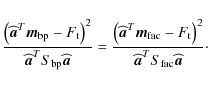
Having the correct parameters in hand, LDA could then be carried out to find their linear combination that best
discriminates the training set classes. Explicitely, we searched for the axis vector
![]() that
maximizes Fischer's separability criterion (as introduced in the original work of Fischer 1936) in the
parameter space
that
maximizes Fischer's separability criterion (as introduced in the original work of Fischer 1936) in the
parameter space
![]() :
:
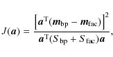
where the superscript T denotes transpose,
The DFs of the discriminant parameters (Fig. 8 right column) and of the variable F (Fig. 9d) also give a good visual estimate of the amount of overlap between the training set classes. An
intuitive measure of the discriminant power of a parameter could then be given by the ratio between the number of
features contained in the overlapping part of the DFs and the total number of training
set features. This ratio already takes a fairly low value of 0.07 for ![]() (
(![]() ), and goes down to 0.042 for F. However, such a measure is statistically poor compared to J, since it mostly relies on the outliers contained in the tails of the DFs (only 28 and 17 features for
), and goes down to 0.042 for F. However, such a measure is statistically poor compared to J, since it mostly relies on the outliers contained in the tails of the DFs (only 28 and 17 features for
![]() )
and F, respectively), whereas Jtakes advantage of the full parameter distributions.
)
and F, respectively), whereas Jtakes advantage of the full parameter distributions.
The overlap of the DF of
![]() )
and the particular skewness of the DF of faculae towards small areas arises from our MLT segmentation. To investigate the influence of the MLT levels on the DFs of the dicriminant parameters and on LDA, we carried out tests with fewer MLT levels over the same training set. We
found that the skewness of the DF of
)
and the particular skewness of the DF of faculae towards small areas arises from our MLT segmentation. To investigate the influence of the MLT levels on the DFs of the dicriminant parameters and on LDA, we carried out tests with fewer MLT levels over the same training set. We
found that the skewness of the DF of ![]() (
(
![]() )
for faculae is in major part due to their segmentation
into fine striations. It should be noticed that the DF of log(
)
for faculae is in major part due to their segmentation
into fine striations. It should be noticed that the DF of log(![]() )
is less skewed, because the characteristic profiles of these striated faculae are mostly retrieved along the long dimension of the striations (owing to their individual orientation, see Sect. 3.2), which makes
)
is less skewed, because the characteristic profiles of these striated faculae are mostly retrieved along the long dimension of the striations (owing to their individual orientation, see Sect. 3.2), which makes ![]() a robust parameter to
distinguish them from BPs. However, the coarser segmentation of the tests has the undesired effect that a part of
the features are undersegmented, which leads to lower values of J for all parameters as well as for the
discriminant variable F. Due to the merging of BPs into chains and ribbons, their DFs are particularly affected
and become skewed towards larger
a robust parameter to
distinguish them from BPs. However, the coarser segmentation of the tests has the undesired effect that a part of
the features are undersegmented, which leads to lower values of J for all parameters as well as for the
discriminant variable F. Due to the merging of BPs into chains and ribbons, their DFs are particularly affected
and become skewed towards larger
![]() and smaller
and smaller ![]() .
For
.
For ![]() and
and ![]() ,
this is
probably a consequence of the misorientation of merged features when retrieving the characteristic profiles. We
believe that those tests confirm our appropriate choice of MLT levels for the purpose of further discriminating
between individual BPs and faculae.
,
this is
probably a consequence of the misorientation of merged features when retrieving the characteristic profiles. We
believe that those tests confirm our appropriate choice of MLT levels for the purpose of further discriminating
between individual BPs and faculae.
We stress that the procedure of orienting the features prior to the retrieval of their contrast profiles, as described in Sect. 3.2, is an essential ingredient to obtain discriminant parameters based on those profiles. In early stages of this work, profiles were only retrieved along the direction perpendicular to the closest limb, and the ensuing overlap of the DFs was significantly larger.
Finally, it should be noted that the values of these photometric discriminant parameters all depend to some extent
on the spatial resolution. ![]() is probably the most sensitive in that respect, but it has the least weight
in the variable F due to its lower value of J (see Table 2). This points to the
requirement of having a dataset of roughly constant resolution, a condition met by our selection of images (Sect. 2.1).
is probably the most sensitive in that respect, but it has the least weight
in the variable F due to its lower value of J (see Table 2). This points to the
requirement of having a dataset of roughly constant resolution, a condition met by our selection of images (Sect. 2.1).
Table 2: J values associated with each discriminant parameter, and for the variable F obtained by linear combination of the three parameters.
4 Classification results and discussion
4.1 Hard threshold vs. reject option
To build an assignment rule, we made the usual choice of a threshold value ![]() at equal ``standardized''
distance from the class means (Mahalanobis 1936; Murtagh & Heck 1987), namely:
at equal ``standardized''
distance from the class means (Mahalanobis 1936; Murtagh & Heck 1987), namely:
This threshold is drawn on the density function histogram of F in Fig. 9d.
In a first step, a single hard threshold equal to ![]() was used to classify all the segmented features as BPs or faculae by measuring their values of F. Because we are not interested in absolute numbers, but rather in the relative distribution of BPs and faculae, we define the classified fractions of BPs and faculae as:
was used to classify all the segmented features as BPs or faculae by measuring their values of F. Because we are not interested in absolute numbers, but rather in the relative distribution of BPs and faculae, we define the classified fractions of BPs and faculae as:
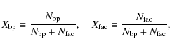
where
![\begin{figure}
\par\includegraphics[width=16cm]{1117fig10.eps}\par
\end{figure}](/articles/aa/full_html/2009/28/aa11117-08/img114.png) |
Figure 10:
a) CLV of relative fractions of BPs (`` |
| Open with DEXTER | |
As already stated at the end of Sect. 3.1, there is a continuous spectrum of intermediate
features between BPs and faculae that cannot be reasonably identified as belonging to one class or the other.
The only way to avoid the erroneous classification of these features is to exclude them from the statistics by
introducing a so-called ``reject option'' (Hand 1981), in the form of a rejection range in F centered about
![]() .
Assuming that all intermediate features fall within the rejection range, the relations between
classified and true numbers
.
Assuming that all intermediate features fall within the rejection range, the relations between
classified and true numbers
![]() ,
,
![]() (such as would be recognized by eye) at
each disk position are:
(such as would be recognized by eye) at
each disk position are:
where
Under the full rejection of intermediate features, the classified fractions then become:
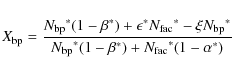
for BPs and similarly for faculae. Note that if the training set is representative and the misclassification rates can be considered negligible, relation 8 further simplifies to
Compared with the CLV of
![]() and
and
![]() obtained with a hard threshold, the difference between
obtained with a hard threshold, the difference between
![]() and
and
![]() at each
at each
![]() is now systematically larger (except for
is now systematically larger (except for
![]() ). This is probably an effect of the contamination by intermediate features in the hard
threshold case, because such features are assigned roughly equally to each class, so that they have the tendency to
equalize
). This is probably an effect of the contamination by intermediate features in the hard
threshold case, because such features are assigned roughly equally to each class, so that they have the tendency to
equalize
![]() and
and
![]() .
The difference between
.
The difference between
![]() and
and
![]() is particularly
large for
is particularly
large for
![]() and for the limbward data points at
and for the limbward data points at
![]() .
This is
likely to be attributed to the larger misclassification errors in the hard threshold method than with the reject
option. Indeed, as can be seen from relation (4), the misclassification errors also tend to
overestimate the number of BPs near the limb where faculae dominate, while underestimating it near disk center,
and vice versa for faculae. To estimate the true misclassification rates, we computed the apparent
misclassification rates
.
This is
likely to be attributed to the larger misclassification errors in the hard threshold method than with the reject
option. Indeed, as can be seen from relation (4), the misclassification errors also tend to
overestimate the number of BPs near the limb where faculae dominate, while underestimating it near disk center,
and vice versa for faculae. To estimate the true misclassification rates, we computed the apparent
misclassification rates
![]() by reclassifying the training set, assuming as before that the latter
adequately represents the true populations. With the chosen rejection range, we obtained
by reclassifying the training set, assuming as before that the latter
adequately represents the true populations. With the chosen rejection range, we obtained
![]() ,
which is an order of magnitude smaller than in the the hard threshold case and should be reflected in the true
rates as well
,
which is an order of magnitude smaller than in the the hard threshold case and should be reflected in the true
rates as well![]() .
.
We shall now elaborate on the validity of the aforementioned assumptions, and further justify the use of
a reject option as opposed to the hard threshold classification. A subtle source of error is the departure of the actual populations from the training set ones, causing
![]() .
To evaluate the importance of this effect, we have varied
.
To evaluate the importance of this effect, we have varied ![]() in the range (0.2, 0.5), which should in that case induce unequal
variation of
in the range (0.2, 0.5), which should in that case induce unequal
variation of
![]() and
and
![]() and consequently different variations of
and consequently different variations of
![]() and
and
![]() (cf. Eq. (8)). By the same token, this allowed us to check if intermediate features were still wrongly classified as BPs or faculae for
(cf. Eq. (8)). By the same token, this allowed us to check if intermediate features were still wrongly classified as BPs or faculae for
![]() ,
as the separation between
,
as the separation between
![]() and
and
![]() should then increase with
should then increase with ![]() .
But instead, we observed both positive and negative fluctuations of
.
But instead, we observed both positive and negative fluctuations of
![]() and
and
![]() ,
indicating that most intermediate features were indeed rejected, and that the true rejection rates were nearly equal for BPs and faculae. As those fluctuations were always less
than 0.05, we chose this value as an upper limit on the error induced by uneven actual rejection rates, and
represented it by the symmetric error bars in Fig. 10b. To compare the effect of rejection at
the various disk positions, we overplotted in Fig. 10b the fraction of rejected
features with respect to the total number of features
,
indicating that most intermediate features were indeed rejected, and that the true rejection rates were nearly equal for BPs and faculae. As those fluctuations were always less
than 0.05, we chose this value as an upper limit on the error induced by uneven actual rejection rates, and
represented it by the symmetric error bars in Fig. 10b. To compare the effect of rejection at
the various disk positions, we overplotted in Fig. 10b the fraction of rejected
features with respect to the total number of features
![]() .
The relative constancy of
.
The relative constancy of
![]() is reassuring, and reflects the self-similarity of the actual BPs and faculae
populations at various
is reassuring, and reflects the self-similarity of the actual BPs and faculae
populations at various
![]() (as far as F is concerned). It also gives an indication about the
number of intermediate features, as in absence of them we would have
(as far as F is concerned). It also gives an indication about the
number of intermediate features, as in absence of them we would have
![]() ,
using as before
,
using as before
![]() together with the relation (6). As
can be seen, the fraction of rejected features fluctuates around 0.4, indicating a significant fraction of
intermediate features
together with the relation (6). As
can be seen, the fraction of rejected features fluctuates around 0.4, indicating a significant fraction of
intermediate features
![]() ,
which further justifies the introduction of the
rejection range.
,
which further justifies the introduction of the
rejection range.
From a methodological point of view, despite the qualitative resemblance of the CLVs obtained with the
hard threshold and with the reject option, the first method is open to criticism due to the large amount of
intermediate features. A hard threshold is in this sense self-contradictory, as it tries to assign these features
to classes whose reference (the training set) does not represent them. By contrast, if these features are
properly rejected, and if the assumptions of negligible misclassification rates and representative training set
(
![]() )
are justified, the reject option method has the elegance that the classified
fractions closely approximate the true ones.
)
are justified, the reject option method has the elegance that the classified
fractions closely approximate the true ones.
Lastly, the results obtained here do not only depend on the choice of the training set, but also on the choice of the classification method. Fischer's LDA implicitely assumes similar covariance matrices for the classes, which is not quite true in our case, as can be seen from the different shapes of the BPs and faculae ``clouds'' in their 2D projections (Fig. 9). We then implemented a ``class-dependent'' LDA, taking into account the difference in covariance matrices and deriving different discriminant axes for the two classes (Balakrishnama et al. 1999). However, the difference in the relative fractions obtained was insignificant, thereby indicating that the covariance matrices of our chosen parameters were suitable for Fischer's LDA.
4.2 Discussion
To assess the validity of the proposed method, the obtained results can be compared with the observations of BPs
and faculae at various ![]() available in the literature. To help the comparison as well as to give a visual
idea of which features were classified as BPs and faculae, Figs. 11-13 show their contours overlaid on the G-band images at
available in the literature. To help the comparison as well as to give a visual
idea of which features were classified as BPs and faculae, Figs. 11-13 show their contours overlaid on the G-band images at
![]() ,
,
![]() (same images as in Figs. 1 and 2), and
(same images as in Figs. 1 and 2), and
![]() respectively. Our results are consistent with recent high-resolution observations from Berger et al. (2007), who noticed the presence of disk-center faculae at
respectively. Our results are consistent with recent high-resolution observations from Berger et al. (2007), who noticed the presence of disk-center faculae at
![]() ,
very few intergranular BPs at
,
very few intergranular BPs at
![]() ,
and a mixture of both features at
,
and a mixture of both features at
![]() .
The presence of some ``intergranular brightenings'' around
.
The presence of some ``intergranular brightenings'' around
![]() also has been reported by Lites et al. (2004), and Hirzberger & Wiehr (2005) have clearly observed the coexistence of BPs
and faculae at
also has been reported by Lites et al. (2004), and Hirzberger & Wiehr (2005) have clearly observed the coexistence of BPs
and faculae at
![]() .
This suggests the validity of our classification method, although this should be
confirmed in the future by using datasets with co-temporal magnetic vector information.
.
This suggests the validity of our classification method, although this should be
confirmed in the future by using datasets with co-temporal magnetic vector information.
Although our CLV cannot be generalized due to the limited statistics of the present dataset and the coarse sampling of the ![]() range, it allows us to constrain the
range, it allows us to constrain the ![]() interval where the transition from BPs to faculae occurs. In this respect, the CLV also exhibits a plateau in the range
interval where the transition from BPs to faculae occurs. In this respect, the CLV also exhibits a plateau in the range
![]() ,
indicating that
BPs may still be found in that range, but progressively disappear closer to the limb, probably affected by the
foreground granular obscuration (Auffret & Muller 1991). This plateau can also be attributed to the slower variation of
the heliocentric angle in that
,
indicating that
BPs may still be found in that range, but progressively disappear closer to the limb, probably affected by the
foreground granular obscuration (Auffret & Muller 1991). This plateau can also be attributed to the slower variation of
the heliocentric angle in that ![]() range (
range (
![]() )
compared to the centerward range
)
compared to the centerward range
![]() (
(
![]() ). Conversely, faculae appear to be present at all disk
positions, except for the inner third of the disk where
). Conversely, faculae appear to be present at all disk
positions, except for the inner third of the disk where ![]() .
Hence, in contrast to full-disk images in
which faculae patches are only prominent closer to the limb, at high resolution faculae are conspicuous features
of active-region plages at all disk positions.
.
Hence, in contrast to full-disk images in
which faculae patches are only prominent closer to the limb, at high resolution faculae are conspicuous features
of active-region plages at all disk positions.
The overall dominance of faculae in our dataset as well as the presence of BPs at relatively small ![]() values (
values (
![]() )
cannot be understood in terms of the conventional ``hot wall'' picture, if we consider only vertical flux tubes and varying viewing angles with disk position. The most straightforward alternative is to
invoke inclined fields (e.g. due to swaying motions), whereby BPs would arise from flux tubes aligned along the line of sight and faculae from flux tubes inclined with respect to it. Again, such an hypothesis should be verified with the help of magnetic vector data.
)
cannot be understood in terms of the conventional ``hot wall'' picture, if we consider only vertical flux tubes and varying viewing angles with disk position. The most straightforward alternative is to
invoke inclined fields (e.g. due to swaying motions), whereby BPs would arise from flux tubes aligned along the line of sight and faculae from flux tubes inclined with respect to it. Again, such an hypothesis should be verified with the help of magnetic vector data.
From here on, we discuss the assets and weaknesses of the proposed method, as well as its applicability. A key point of the method resides in the orientation of individually segmented features so as to
retrieve characteristic profiles (see Sect. 3.2). This procedure makes the method applicable at different
![]() (due to the diverse orientations of BPs and faculae), and thereby offers the possibility of studying the transition from BPs to faculae as
(due to the diverse orientations of BPs and faculae), and thereby offers the possibility of studying the transition from BPs to faculae as ![]() varies. In the considered
varies. In the considered ![]() range at
least, the orientation process makes the discriminant parameters roughly
range at
least, the orientation process makes the discriminant parameters roughly ![]() -invariant, thus allowing LDA to be
applied to the whole dataset at once (cf. Sect. 3.3). LDA itself has the advantage of being fairly simple to implement, and of making few assumptions on the distribution properties of the discriminant parameters (see Sect. 3.4). It nevertheless requires the careful preselection of a training set, a
crucial step that can potentially bias the classification. But the principal weakness of the current method lies
in the use of photometric information only, allowing a limited number of discriminant parameters to be
defined. This induces the following pitfall: faculae ``sitting'' on very small granules (fragments, abnormal
granulation) are basically indistinguishible from BPs as far as our parameters are concerned. Several instances
appear in Figs. 12 and 13, where such small faculae are either rejected or misclassified. The method could be improved by the inclusion of discriminant parameters coming from polarimetric maps, provided that BPs and faculae exhibit sufficiently different magnetic properties.
-invariant, thus allowing LDA to be
applied to the whole dataset at once (cf. Sect. 3.3). LDA itself has the advantage of being fairly simple to implement, and of making few assumptions on the distribution properties of the discriminant parameters (see Sect. 3.4). It nevertheless requires the careful preselection of a training set, a
crucial step that can potentially bias the classification. But the principal weakness of the current method lies
in the use of photometric information only, allowing a limited number of discriminant parameters to be
defined. This induces the following pitfall: faculae ``sitting'' on very small granules (fragments, abnormal
granulation) are basically indistinguishible from BPs as far as our parameters are concerned. Several instances
appear in Figs. 12 and 13, where such small faculae are either rejected or misclassified. The method could be improved by the inclusion of discriminant parameters coming from polarimetric maps, provided that BPs and faculae exhibit sufficiently different magnetic properties.
We conclude by drawing attention to precautions that should be taken in applying our method to other datasets. Having a fairly homogeneous and high spatial resolution is an essential requirement, as the values of all parameters
![]() ,
,
![]() and
and ![]() depend on it. A variable resolution would cause the values of the parameters to vary throughout the dataset (between different images or even accross the field of view), thus preventing a well-defined discriminant variable and a unique BP/faculae threshold from being obtained. For a
dataset with a constant but different resolution, the method would in principle still be valid, but the values of
the parameters and of the class threshold would differ. However, degrading datasets of variable resolution to a
constant lower one would reduce the contrast of features (loss of statistics due to the contrast threshold), and
blur the local contrast depressions, so that it would become difficult to separate adjacent BPs and faculae
striations. The method would also lose in efficiency due to the misorientation of merged features (cf. Sect. 3.2).
Finally, care
should be taken in applying unchanged the herein-derived discriminant F and its threshold value to other
datasets. If the current method is applied to a dataset of slightly different resolution (or with a different
amount of straylight), wavelengths (e.g. CN-band, Zakharov et al. 2007) or
depend on it. A variable resolution would cause the values of the parameters to vary throughout the dataset (between different images or even accross the field of view), thus preventing a well-defined discriminant variable and a unique BP/faculae threshold from being obtained. For a
dataset with a constant but different resolution, the method would in principle still be valid, but the values of
the parameters and of the class threshold would differ. However, degrading datasets of variable resolution to a
constant lower one would reduce the contrast of features (loss of statistics due to the contrast threshold), and
blur the local contrast depressions, so that it would become difficult to separate adjacent BPs and faculae
striations. The method would also lose in efficiency due to the misorientation of merged features (cf. Sect. 3.2).
Finally, care
should be taken in applying unchanged the herein-derived discriminant F and its threshold value to other
datasets. If the current method is applied to a dataset of slightly different resolution (or with a different
amount of straylight), wavelengths (e.g. CN-band, Zakharov et al. 2007) or ![]() range, the values of the
segmentation thresholds should first be adapted (the same holds for the identification criteria of the
``grey-lane'' BPs), and the training set selection must then be repeated (as well as the subsequent steps of the
method thereof). Under different conditions, the ensuing values of the discriminant parameters will be different,
and consequently LDA will yield a different linear combination for the discriminant variable and a different
threshold.
range, the values of the
segmentation thresholds should first be adapted (the same holds for the identification criteria of the
``grey-lane'' BPs), and the training set selection must then be repeated (as well as the subsequent steps of the
method thereof). Under different conditions, the ensuing values of the discriminant parameters will be different,
and consequently LDA will yield a different linear combination for the discriminant variable and a different
threshold.
5 Summary and outlook
We have developed a photometric method based on Linear Discriminant Analysis (LDA) to discriminate
between individual Bright Points (BPs) and faculae, observed at high resolution over a range of heliocentric
angles. We first demonstrated the feasibility of an automated segmentation for both individual BPs and faculae
at various disk positions, based on joint G-band and continuum photometric information only. For each segmented
feature, a ``characteristic G-band contrast profile'' was retrieved along a specific direction, by properly
orienting the feature using its ``contrast moment of inertia''. Three physical parameters were then identified to
be good discriminants between BPs and faculae at all disk positions of our dataset: the width and slope of the
contrast profiles, as well as the apparent area defined by the segmentation map. Linear discriminant
analysis was then performed on a visually-selected reference set of BPs and faculae, yielding a single linear
combination of the parameters as the discriminant variable for all disk positions. Using an appropriate threshold and
rejection range on this variable, all the segmented features were ultimately classified and the relative
fractions of BPs and faculae at each disk position of our dataset were computed. The resulting CLV of these
fractions is mostly faculae-dominated except for ![]() ,
i.e. close to disk center. This is in agreement
with previous observations, thus suggesting the validity of the presented method. We propose that these
ubiquitous faculae are produced by a hot-wall effect through inclined fields.
,
i.e. close to disk center. This is in agreement
with previous observations, thus suggesting the validity of the presented method. We propose that these
ubiquitous faculae are produced by a hot-wall effect through inclined fields.
Using our classification method, we plan to present more statistical results concerning photometric properties of BPs and faculae (such as contrast and morphology) in a forthcoming paper. A similar classification study should in future also be performed on a high-resolution dataset with magnetic field vector information, in order to determine the magnetic properties of BPs and faculae separately and further validate the method. Such datasets can now be obtained from ground-based imaging polarimeters such as the GFPI (Puschmann et al. 2006), CRISP (Scharmer et al. 2008), or IBIS (Cavallini 2006), and in the near future from the SUNRISE (Gandorfer et al. 2007) stratospheric balloon-borne observatory. Through their seeing-free quality, the images of SUNRISE will be very promising for the application of our method, as they will naturally satisfy its requirement of homogeneous spatial resolution. In particular, a comparison of the classification results with the field inclinations retrieved by Stokes profile inversions could be particularly interesting to verify the hypothetical association of faculae with inclined fields. Ultimately, a similar classification should be performed on synthetic images computed from 3D MHD simulation boxes at various angles. A comparison with the classification obtained from observational data would then give more physical insight into the relationship between BPs and faculae on one hand, and provide novel constraints for the models on the other hand.
Acknowledgements
We are grateful to F. Kneer, E. Wiehr, O. Steiner, F. Murtagh, M. Schüssler and W. Stahel for their interest in the present work and their fruitful comments. We thank as well P. Sütterlin for having provided the basis of our image warping code. This work was partly supported by the WCU grant No. R31-10016 from the Korean Ministry of Education, Science and Technology. Finally, our gratitude is directed towards D. Schmitt and the ``Solar System School'', in which frame this research could be carried out.
References
- Antoine, J.-P., Demanet, L., Hochedez, J.-F., et al. 2002, Physicalia, 24, 93 (In the text)
- Auffret, H., & Muller, R. 1991, A&A, 246, 264 [NASA ADS] (In the text)
- Balakrishnama, S., Ganapathiraju, A., & Picone, J. 1999, in Proceedings IEEE Southeastcon'99. Technology on the Brink of 2000., 78 (In the text)
- Barnes, G., Leka, K. D., Schumer, E. A., & Della-Rose, D. J. 2007, Space Weather, 5
- Berger, T. E., Schrijver, C. J., Shine, R. A., et al. 1995, ApJ, 454, 531 [NASA ADS] [CrossRef]
- Berger, T. E., Löfdahl, M. G., Shine, R. S., & Title, A. M. 1998, ApJ, 495, 973 [NASA ADS] [CrossRef] (In the text)
- Berger, T. E., Rouppe van der Voort, L., & Löfdahl, M. 2007, ApJ, 661, 1272 [NASA ADS] [CrossRef]
- Berger, T. E., & Title, A. M. 2001, ApJ, 553, 449 [NASA ADS] [CrossRef] (In the text)
- Bovelet, B., & Wiehr, E. 2001, Sol. Phys., 201, 13 [NASA ADS] [CrossRef]
- Bovelet, B., & Wiehr, E. 2003, A&A, 412, 249 [NASA ADS] [CrossRef] [EDP Sciences]
- Bovelet, B., & Wiehr, E. 2007, Sol. Phys., 243, 121 [NASA ADS] [CrossRef]
- Carlsson, M., Stein, R. F., Nordlund, Å., & Scharmer, G. B. 2004, ApJ, 610, L137 [NASA ADS] [CrossRef]
- Cavallini, F. 2006, Sol. Phys., 236, 415 [NASA ADS] [CrossRef] (In the text)
- De Pontieu, B., Carlsson, M., Stein, R., et al. 2006, ApJ, 646, 1405 [NASA ADS] [CrossRef] (In the text)
- Dunn, R. B., & Zirker, J. B. 1973, Sol. Phys., 33, 281 [NASA ADS]
- Fischer, R. A. 1936, Annals of Eugenics, 7, 179 (In the text)
- Fligge, M., Solanki, S. K., Unruh, Y. C., Fröhlich, C., & Wehrli, C. 1998, A&A, 335, 709 [NASA ADS]
- Gandorfer, A. M., Solanki, S. K., Barthol, P., et al. & the SUNRISE team 2007, in Modern Solar Facilities - Advanced Solar Science, ed. F. Kneer, K. G. Puschmann, & A. D. Wittmann (Universitätsverlag Göttingen), 69 (In the text)
- Hand, D. 1981, Discrimination and Classification (New York: Wiley) (In the text)
- Heck, A., & Murtagh, F., ed. 1989, Knowledge-Based Systems in Astronomy, Lect. Notes Phys. (Berlin: Springer Verlag), 329, (In the text)
- Hirzberger, J., & Wiehr, E. 2005, A&A, 438, 1059 [NASA ADS] [CrossRef] [EDP Sciences] (In the text)
- Keller, C. U., Schüssler, M., Vögler, A., & Zakharov, V. 2004, ApJ, 607, L59 [NASA ADS] [CrossRef]
- Kenney, J. F., & Keeping, E. S. 1962, Mathematics of Statistics, Pt. 1, 3rd edn (Princeton, NJ: Van Nostrand) (In the text)
- Knölker, M., Schüssler, M., & Weisshaar, E. 1988, A&A, 194, 257 [NASA ADS]
- Knölker, M., Grossmann-Doerth, U., Schüssler, M., & Weisshaar, E. 1991, Adv. Space Res., 11, 285 [NASA ADS] [CrossRef]
- Krivova, N. A., Solanki, S. K., Fligge, M., & Unruh, Y. C. 2003, A&A, 399, L1 [NASA ADS] [CrossRef] [EDP Sciences]
- Langhans, K., Schmidt, W., & Tritschler, A. 2002, A&A, 394, 1069 [NASA ADS] [CrossRef] [EDP Sciences]
- Lean, J., & Foukal, P. 1988, Science, 240, 906 [NASA ADS] [CrossRef]
- Leka, K. D., & Barnes, G. 2003, ApJ, 595, 1296 [NASA ADS] [CrossRef]
- Limpert, E., Stahel, W., & Abbt, M. 2001, BioSc., 427, 341 [CrossRef] (In the text)
- Lites, B. W., Scharmer, G. B., Berger, T. E., & Title, A. M. 2004, Sol. Phys., 221, 65 [NASA ADS] [CrossRef]
- Mahalanobis, P. C. 1936, Proc. National Inst. Sci. India, 12
- Mehltretter, J. P. 1974, Sol. Phys., 38, 43 [NASA ADS] [CrossRef]
- Muller, R. 1975, Sol. Phys., 45, 105 [NASA ADS] [CrossRef] (In the text)
- Muller, R., & Roudier, T. 1984, Sol. Phys., 94, 33 [NASA ADS] [CrossRef]
- Murtagh, F., & Heck, A. 1987, Multivariate Data Analysis (Kluwer Academic Publishers, Dordrecht) (In the text)
- Neckel, H., & Labs, D. 1994, Sol. Phys., 153, 91 [NASA ADS] [CrossRef] (In the text)
- Puschmann, K. G., Kneer, F., Seelemann, T., & Wittmann, A. D. 2006, A&A, 451, 1151 [NASA ADS] [CrossRef] [EDP Sciences] (In the text)
- Sánchez Almeida, J., Asensio Ramos, A., Trujillo Bueno, J., & Cernicharo, J. 2001, ApJ, 555, 978 [NASA ADS] [CrossRef] (In the text)
- Scharmer, G. B., Narayan, G., Hillberg, T., et al. 2008, ApJ, 689, L69 [NASA ADS] [CrossRef] (In the text)
- Schüssler, M. 1992, in NATO Advanced Study Institute Series C Proc. 373: The Sun: A Laboratory for Astrophysics, ed. J. T. Schmelz, & J. C. Brown, 191
- Schüssler, M., Shelyag, S., Berdyugina, S., Vögler, A., & Solanki, S. K. 2003, ApJ, 597, L173 [NASA ADS] [CrossRef]
- Shelyag, S., Schüssler, M., Solanki, S. K., Berdyugina, S. V., & Vögler, A. 2004, A&A, 427, 335 [NASA ADS] [CrossRef] [EDP Sciences]
- Smith, Jr., J. B., Neidig, D. F., Wiborg, P. H., et al. 1996, in Solar Drivers of the Interplanetary and Terrestrial Disturbances, ed. K. S. Balasubramaniam, S. L. Keil, & R. N. Smartt, ASP Conf. Ser., 95, 55
- Solanki, S. K. 1993, Space Sci. Rev., 63, 1 [NASA ADS] [CrossRef]
- Solanki, S. K., Inhester, B., & Schüssler, M. 2006, Rep. Prog. Phys., 69, 563 [NASA ADS] [CrossRef]
- Spruit, H. C. 1976, Sol. Phys., 50, 269 [NASA ADS] [CrossRef]
- Steiner, O. 2005, A&A, 430, 691 [NASA ADS] [CrossRef] [EDP Sciences]
- Stenflo, J. O. 1973, Sol. Phys., 32, 41 [NASA ADS] [CrossRef] (In the text)
- Title, A. M., & Berger, T. E. 1996, ApJ, 463, 797 [NASA ADS] [CrossRef]
- Title, A. M., Tarbell, T. D., & Topka, K. P. 1987, ApJ, 317, 892 [NASA ADS] [CrossRef] (In the text)
- Tung, K., & Camp, D. 2008, J. Geophys. Res., 113 (In the text)
- Vögler, A., Shelyag, S., Schüssler, M., Cattaneo, F., Emonet, T., & Linde, T. 2005, A&A, 429, 335 [NASA ADS] [CrossRef] [EDP Sciences] (In the text)
- Walton, S. R., Preminger, D. G., & Chapman, G. A. 2003, ApJ, 590, 1088 [NASA ADS] [CrossRef]
- Wilson, P. R. 1981, Sol. Phys., 69, 9 [NASA ADS] [CrossRef]
- Zakharov, V., Gandorfer, A., Solanki, S. K., & Löfdahl, M. 2007, A&A, 461, 695 [NASA ADS] [CrossRef] [EDP Sciences] (In the text)
Online Material
![\begin{figure}
\par\includegraphics[width=17cm]{1117fig11.eps}
\end{figure}](/articles/aa/full_html/2009/28/aa11117-08/img152.png) |
Figure 11:
G-band image at
|
| Open with DEXTER | |
![\begin{figure}
\par\includegraphics[width=17cm]{1117fig12.eps}
\end{figure}](/articles/aa/full_html/2009/28/aa11117-08/img153.png) |
Figure 12:
G-band image at
|
| Open with DEXTER | |
![\begin{figure}
\par\includegraphics[width=16cm,clip]{1117fig13.eps}
\end{figure}](/articles/aa/full_html/2009/28/aa11117-08/img154.png) |
Figure 13:
G-band image at
|
| Open with DEXTER | |
![\begin{figure}
\par\includegraphics[width=16cm,clip]{1117fig14.eps}
\end{figure}](/articles/aa/full_html/2009/28/aa11117-08/img155.png) |
Figure 14:
Original G-band image at
|
| Open with DEXTER | |
Footnotes
- ... faculae
- Figures 11-14 are only available in electronic form at http://www.aanda.org
- ... features
- Involving pixels with lower contrast yields poorer results, as these are often associated with granulation in the case of faculae, and thus do not carry information about the orientation of the facular brightening itself.
- ... log-transforms
- This was partly expected, as the width of magnetic bright points has been observed to be log-normally distributed (Berger et al. 1995).
- ... well
- As these are only optimistic estimates fo the true misclassification rates, we implemented a ``leave-one-out'' method on the training set (Murtagh & Heck 1987; Hand 1981), which nevertheless gave the same results as the simple reclassification (probably due to the fairly large size of the training set).
All Tables
Table 1: Dataset specifications.
Table 2: J values associated with each discriminant parameter, and for the variable F obtained by linear combination of the three parameters.
All Figures
| |
Figure 1:
G-band image of NOAA 0669 at
|
| Open with DEXTER | |
| In the text | |
| |
Figure 2:
G-band image of NOAA 0671
|
| Open with DEXTER | |
| In the text | |
| |
Figure 3:
|
| Open with DEXTER | |
| In the text | |
| |
Figure 4:
Maximum G-band contrast values (small crosses) of all features segmented only with a difference threshold
|
| Open with DEXTER | |
| In the text | |
| |
Figure 5:
Orientation of an individual feature in its local x/y coordinate frame. a) Zoom window surrounding
the feature in the original G-band image. The cross indicates the location of the contrast maximum; b) isolated
feature as delimited by the segmentation map. The pixels having
|
| Open with DEXTER | |
| In the text | |
| |
Figure 6:
Local frame orientation and G-band contrast profiles and of a typical facula (left) and a typical BP (right). Top windows: orientation of the features in their local x/y coordinate frames, where the black lines delimit the pixels having
|
| Open with DEXTER | |
| In the text | |
| |
Figure 7:
Characteristic profiles (thick lines) of BPs a, b) and intermediate features c, d) surrounded by one or two ``grey'' lanes. On the grey lane sides, the characteristic profiles have been linearly extrapolated from the half-max level (``+'') to
|
| Open with DEXTER | |
| In the text | |
| |
Figure 8:
Left column: mean values and standard deviations of the three parameters for the BPs (`` |
| Open with DEXTER | |
| In the text | |
| |
Figure 9:
a-c) 2D projections of the 3D training set vectors
|
| Open with DEXTER | |
| In the text | |
| |
Figure 10:
a) CLV of relative fractions of BPs (`` |
| Open with DEXTER | |
| In the text | |
| |
Figure 11:
G-band image at
|
| Open with DEXTER | |
| In the text | |
| |
Figure 12:
G-band image at
|
| Open with DEXTER | |
| In the text | |
| |
Figure 13:
G-band image at
|
| Open with DEXTER | |
| In the text | |
| |
Figure 14:
Original G-band image at
|
| Open with DEXTER | |
| In the text | |
Copyright ESO 2009
Current usage metrics show cumulative count of Article Views (full-text article views including HTML views, PDF and ePub downloads, according to the available data) and Abstracts Views on Vision4Press platform.
Data correspond to usage on the plateform after 2015. The current usage metrics is available 48-96 hours after online publication and is updated daily on week days.
Initial download of the metrics may take a while.