| Issue |
A&A
Volume 501, Number 3, July III 2009
|
|
|---|---|---|
| Page(s) | 865 - 877 | |
| Section | Cosmology (including clusters of galaxies) | |
| DOI | https://doi.org/10.1051/0004-6361/200811570 | |
| Published online | 13 May 2009 | |
A comprehensive study of large-scale structures in the GOODS-SOUTH field up to
 2.5
2.5
S. Salimbeni1,2 - M. Castellano3,2 - L. Pentericci2 - D. Trevese3 - F. Fiore2 - A. Grazian2 - A. Fontana2 - E. Giallongo2 - K. Boutsia2 - S. Cristiani4 - C. De Santis5,6 - S. Gallozzi2 - N. Menci2 - M. Nonino4 - D. Paris2 - P. Santini2 - E. Vanzella4
1 - Department of Astronomy, University of Massachusetts, 710 North Pleasant Street, Amherst, MA 01003, USA
2 - INAF - Osservatorio Astronomico di Roma, via Frascati 33,
00040 Monteporzio (RM), Italy
3 - Dipartimento di Fisica,
Universitá di Roma ``La Sapienza'', P.le A. Moro 2, 00185 Roma,
Italy
4 - INAF - Osservatorio Astronomico di Trieste, via G.B. Tiepolo 11, 34131 Trieste, Italy
5 - Dip. di Fisica, Universitá Tor Vergata,
via della Ricerca Scientifica 1,
00133 Roma, Italy
6 - INFN-Roma Tor Vergata,
via della Ricerca Scientifica 1,
00133 Roma, Italy
Received 22 December 2008 / Accepted 21 March 2009
Abstract
Aims. The aim of the present paper is to identify and study the properties and galactic content of groups and clusters in the GOODS-South field up to
![]() ,
and to analyse the physical properties of galaxies as a continuous function of environmental density up to high redshift.
,
and to analyse the physical properties of galaxies as a continuous function of environmental density up to high redshift.
Methods. We used the deep (
![]() ), multi-wavelength GOODS-MUSIC catalogue, which has a 15% of spectroscopic redshifts and accurate photometric redshifts for the remaining fraction. On these data, we applied a (2+1)D algorithm, previously developed by our group, that provides an adaptive estimate of the 3D density field. We supported our analysis with simulations to evaluate the purity and the completeness of the cluster catalogue produced by our algorithm.
), multi-wavelength GOODS-MUSIC catalogue, which has a 15% of spectroscopic redshifts and accurate photometric redshifts for the remaining fraction. On these data, we applied a (2+1)D algorithm, previously developed by our group, that provides an adaptive estimate of the 3D density field. We supported our analysis with simulations to evaluate the purity and the completeness of the cluster catalogue produced by our algorithm.
Results. We find several high-density peaks embedded in larger structures in the redshift range 0.4-2.5. From the analysis of their physical properties (mass profile, M200, ![]() ,
,
![]() ,
U-B vs. B diagram), we find that most of them are groups of galaxies, while two are poor clusters with masses a few times
,
U-B vs. B diagram), we find that most of them are groups of galaxies, while two are poor clusters with masses a few times
![]() .
For these two clusters we find from the Chandra 2Ms data an X-ray emission significantly lower than expected from their optical properties, suggesting that the two clusters are either not virialised or are gas poor. We find that the slope of the colour magnitude relation, for these groups and clusters, is constant at least up to
.
For these two clusters we find from the Chandra 2Ms data an X-ray emission significantly lower than expected from their optical properties, suggesting that the two clusters are either not virialised or are gas poor. We find that the slope of the colour magnitude relation, for these groups and clusters, is constant at least up to ![]() .
We also analyse the dependence on environment of galaxy colours, luminosities, stellar masses, ages, and star formations. We find that galaxies in high-density regions are, on average, more luminous and massive than field galaxies up to
.
We also analyse the dependence on environment of galaxy colours, luminosities, stellar masses, ages, and star formations. We find that galaxies in high-density regions are, on average, more luminous and massive than field galaxies up to ![]() .
The fraction of red galaxies increases with luminosity and with density up to
.
The fraction of red galaxies increases with luminosity and with density up to ![]() .
At higher z this dependence on density disappears. The variation of galaxy properties as a function of redshift and density suggests that a significant change occurs at
.
At higher z this dependence on density disappears. The variation of galaxy properties as a function of redshift and density suggests that a significant change occurs at
![]() -2.
-2.
Key words: galaxies: distances and redshifts - galaxies: evolution - galaxies: high-redshift - galaxies: clusters: general - galaxies: fundamental parameters - cosmology: large-scale structure of Universe
1 Introduction
The study of galaxy clusters and of the variation of galaxy properties as a function of the environment are fundamental tools for understanding the formation and evolution of the large-scale structures and of the different galaxy populations, observed both in the local and in the high-redshift Universe. The effects of the environment on galaxy evolution have been studied at progressively higher redshifts through analysis of single clusters (e.g. Rettura et al. 2008; Tran et al. 2005; Mei et al. 2006; Nakata et al. 2005; Menci et al. 2008; Treu et al. 2003), as well as studying the variation of galaxy colours, morphologies, and other physical parameters as a function of projected or 3-dimensional density (e.g. Cooper et al. 2007; Cucciati et al. 2006; Dressler et al. 1997; Blanton et al. 2005; Elbaz et al. 2007). Moreover, the analysis of cluster properties at different wavelengths provides interesting insights into the matter content and evolutionary histories of these structures (Popesso et al. 2007; Lubin et al. 2004; Rasmussen et al. 2006).
A variety of survey techniques have proved effective at finding
galaxy clusters up to ![]() and beyond. The X-ray selected samples
at
and beyond. The X-ray selected samples
at ![]() probe the most massive and dynamically relaxed systems
(e.g., Maughan et al. 2004; Bremer et al. 2006; Lidman et al. 2008; Stanford et al. 2006). Large-area
multicolour surveys, such as the red-sequence survey
(e.g. Gladders & Yee 2005), have collected samples of systems in a
range of evolutionary stages. The mid-IR cameras on board the Spitzer and Akari
satellites has extended the range and power of multicolour surveys,
producing confirmed and candidate clusters up to
probe the most massive and dynamically relaxed systems
(e.g., Maughan et al. 2004; Bremer et al. 2006; Lidman et al. 2008; Stanford et al. 2006). Large-area
multicolour surveys, such as the red-sequence survey
(e.g. Gladders & Yee 2005), have collected samples of systems in a
range of evolutionary stages. The mid-IR cameras on board the Spitzer and Akari
satellites has extended the range and power of multicolour surveys,
producing confirmed and candidate clusters up to
![]() (Goto et al. 2008; Stanford et al. 2005; Eisenhardt et al. 2008). However, most of the previous techniques
present some difficulties in the range
1.5< z <2.5, where we expect
to observe the formation of the red sequence and the first hints of
colour segregation (Cucciati et al. 2006; Kodama et al. 2007). Searching for extended X-ray
sources becomes progressively more difficult at great distances,
because the surface brightness of the X-ray emission fades as
(1+z)4. The sensitivity of surveys exploiting the Sunyaev-Zeldovich (SZ) effect is, at present, insufficient at detecting any known clusters at z > 1
(Carlstrom et al. 2002; Staniszewski et al. 2008). Finally, detecting of galaxy overdensities in surveys using two-dimensional algorithms either requires additional a priori assumptions on galaxy luminosity function (LF), as in the Matched Filter algorithm (Postman et al. 1996), or relies on the presence of a red sequence (Gladders & Yee 2000). Biases produced by these assumptions can
hardly be evaluated at high redshift.
(Goto et al. 2008; Stanford et al. 2005; Eisenhardt et al. 2008). However, most of the previous techniques
present some difficulties in the range
1.5< z <2.5, where we expect
to observe the formation of the red sequence and the first hints of
colour segregation (Cucciati et al. 2006; Kodama et al. 2007). Searching for extended X-ray
sources becomes progressively more difficult at great distances,
because the surface brightness of the X-ray emission fades as
(1+z)4. The sensitivity of surveys exploiting the Sunyaev-Zeldovich (SZ) effect is, at present, insufficient at detecting any known clusters at z > 1
(Carlstrom et al. 2002; Staniszewski et al. 2008). Finally, detecting of galaxy overdensities in surveys using two-dimensional algorithms either requires additional a priori assumptions on galaxy luminosity function (LF), as in the Matched Filter algorithm (Postman et al. 1996), or relies on the presence of a red sequence (Gladders & Yee 2000). Biases produced by these assumptions can
hardly be evaluated at high redshift.
In this context, photometric redshifts obtained from deep multi-band surveys for large samples of galaxies, though with relatively low accuracy if compared to spectroscopic redshifts, can be exploited to detect and study distant structures. In the past few years, several authors (e.g. Mazure et al. 2007; Zatloukal et al. 2007; Eisenhardt et al. 2008; Botzler et al. 2004; van Breukelen et al. 2006; Scoville et al. 2007) have developed or extended known algorithms to take the greater redshift uncertainties into account. We have developed a new algorithm that uses an adaptive estimate of the 3D density field, as described in detail in Trevese et al. (2007). This method combines galaxy angular positions and precise photometric redshifts to estimate the galaxy number density and to detect galaxy over-densities in three dimensions also at z>1, as described in Sect. 3.
Our first application to the K20 survey (Cimatti et al. 2002) detected
two clusters at
![]() and
and ![]() (Trevese et al. 2007),
previously identified through spectroscopy (Gilli et al. 2003; Adami et al. 2005).
We then applied the algorithm to the much larger GOODS-South field,
and in Castellano et al. (2007), elsewhere C07, we reported our
initial results, i.e. the discovery of a forming cluster of galaxies
at
(Trevese et al. 2007),
previously identified through spectroscopy (Gilli et al. 2003; Adami et al. 2005).
We then applied the algorithm to the much larger GOODS-South field,
and in Castellano et al. (2007), elsewhere C07, we reported our
initial results, i.e. the discovery of a forming cluster of galaxies
at
![]() .
.
In this paper we present the application of the algorithm to the
entire GOODS-South area (![]()
![]() ), using the
GOODS-MUSIC catalogue (Grazian et al. 2006a) up to
), using the
GOODS-MUSIC catalogue (Grazian et al. 2006a) up to
![]() ,
to give a
comprehensive description of the large-scale structures in this
field, with a detailed analysis of the physical properties of each
high-density peak. We also study the physical properties of galaxies
as a function of environmental density up to redshift 2.5,
higher than previous similar studies (e.g., Cooper et al. 2007; Cucciati et al. 2006).
,
to give a
comprehensive description of the large-scale structures in this
field, with a detailed analysis of the physical properties of each
high-density peak. We also study the physical properties of galaxies
as a function of environmental density up to redshift 2.5,
higher than previous similar studies (e.g., Cooper et al. 2007; Cucciati et al. 2006).
To validate our technique, we analysed the completeness and
purity of our cluster detection algorithm, up to
![]() ,
through its application to a set of numerically simulated galaxy
catalogues. Besides allowing an assessment of the physical reality
of the structures found in the GOODS field, this analysis provides
the starting point to test the reliability of the algorithm in view
of our plan to apply it to photometric surveys of similar depth but
covering much larger areas.
,
through its application to a set of numerically simulated galaxy
catalogues. Besides allowing an assessment of the physical reality
of the structures found in the GOODS field, this analysis provides
the starting point to test the reliability of the algorithm in view
of our plan to apply it to photometric surveys of similar depth but
covering much larger areas.
The paper is organised as follows. In Sect. 2, we describe the basic features of our dataset. In Sect. 3, we summarise the basic features of the (2+1)D algorithm used in our analysis, and compare it with other methods based on photometric redshifts. In Sect. 4, we show the results of the application of our method to simulated data. In Sect. 5, we present the catalogue of the structures detected and the derived physical properties. In Sect. 6, we study the colour-magnitude diagrams of the detected structures. In Sect. 7, we analyse the physical properties of galaxies as a continuous function of environmental density.
All the magnitudes used in the present paper are in the AB system,
if not otherwise declared. We adopt a cosmology with
![]() ,
,
![]() ,
and
,
and
![]() .
.
2 The GOODS-MUSIC catalogue
We used the multicolour GOODS-MUSIC catalogue (GOODS MUlticolour Southern Infrared Catalogue; Grazian et al. 2006a). This catalogue comprises information in 14 bands (from U band to
![]() )
over an area of about 143.2
)
over an area of about 143.2
![]() .
We used the z850-selected sample (
.
We used the z850-selected sample (
![]() ), which contains
9862 galaxies (after excluding AGNs and galactic stars). About 15% of the galaxies
in the sample have spectroscopic redshift, and for the other galaxies we
used photometric redshifts obtained from a standard
), which contains
9862 galaxies (after excluding AGNs and galactic stars). About 15% of the galaxies
in the sample have spectroscopic redshift, and for the other galaxies we
used photometric redshifts obtained from a standard ![]() minimisation over a large set
of spectral models (see e.g., Fontana et al. 2000). The accuracy of the
photometric redshift is very good, with an rms of 0.03 for the
minimisation over a large set
of spectral models (see e.g., Fontana et al. 2000). The accuracy of the
photometric redshift is very good, with an rms of 0.03 for the
![]() distribution up to redshift z=2. For a detailed description of the catalogue, we refer to Grazian et al. (2006a).
distribution up to redshift z=2. For a detailed description of the catalogue, we refer to Grazian et al. (2006a).
The method we applied to estimate the rest-frame magnitudes and the
other physical parameters (M, SFR, age) is described in previous papers
(e.g., Fontana et al. 2006). Briefly, we used a ![]() minimisation
analysis, comparing the observed SED of each galaxy to synthetic
templates, and the redshift is fixed during the fitting process to
the spectroscopic or photometric redshift derived in
Grazian et al. (2006a). The set of templates is computed with standard
spectral synthesis models (Bruzual & Charlot 2003), chosen to broadly
encompass the variety of star formation histories, metallicities,
and extinctions of real galaxies. For each model of this grid, we
computed the expected magnitudes in our filter set and found
the best-fitting template. From the best-fitting template, we
obtained, for each galaxy, the physical parameters that we used
in the analysis. Clearly, the physical properties are subject
to uncertainties and biases related to the synthetic libraries used
to fit the galaxy SEDs; however, as shown in Fontana et al. (2006), the
extension of the SEDs to mid-IR wavelengths with IRAC tends to
reduce the uncertainties on the derived stellar masses.
For a detailed analysis of the uncertainties on the physical properties we
refer to our previous papers (Fontana et al. 2006; Grazian et al. 2007).
In the present work we also used of the 2Ms X-ray observation of the Chandra Deep Field South
presented by Luo et al. (2008) and of the catalogue of VLA radio sources (1.4 GHz) on the CDFS compiled by Miller et al. (2008).
minimisation
analysis, comparing the observed SED of each galaxy to synthetic
templates, and the redshift is fixed during the fitting process to
the spectroscopic or photometric redshift derived in
Grazian et al. (2006a). The set of templates is computed with standard
spectral synthesis models (Bruzual & Charlot 2003), chosen to broadly
encompass the variety of star formation histories, metallicities,
and extinctions of real galaxies. For each model of this grid, we
computed the expected magnitudes in our filter set and found
the best-fitting template. From the best-fitting template, we
obtained, for each galaxy, the physical parameters that we used
in the analysis. Clearly, the physical properties are subject
to uncertainties and biases related to the synthetic libraries used
to fit the galaxy SEDs; however, as shown in Fontana et al. (2006), the
extension of the SEDs to mid-IR wavelengths with IRAC tends to
reduce the uncertainties on the derived stellar masses.
For a detailed analysis of the uncertainties on the physical properties we
refer to our previous papers (Fontana et al. 2006; Grazian et al. 2007).
In the present work we also used of the 2Ms X-ray observation of the Chandra Deep Field South
presented by Luo et al. (2008) and of the catalogue of VLA radio sources (1.4 GHz) on the CDFS compiled by Miller et al. (2008).
3 The (2+1)D algorithm for the density estimation
To estimate a three-dimensional density, we developed a method that combines the angular position with the photometric redshift of each object. The algorithm is described in detail in Trevese et al. (2007). Here we outline its main features and, in the next section, we present the simulations used to estimate its reliability.
The procedure is designed to automatically take the
probability into account that a galaxy in our survey is physically associated to a given overdensity. This
is obtained by computing the galaxy densities in volumes whose shape is
proportional to positional uncertainties in each dimension (![]() ,
,
![]() ,
and z).
,
and z).
First, we divided the volume of the survey in cells whose extension in
different directions (
![]() )
depends on the relevant positional accuracy and thus are elongated
in the radial direction. We chose the cell sizes small enough to
keep an acceptable spatial resolution, while avoiding a useless
increase in the computing time. We adopted
)
depends on the relevant positional accuracy and thus are elongated
in the radial direction. We chose the cell sizes small enough to
keep an acceptable spatial resolution, while avoiding a useless
increase in the computing time. We adopted
![]() (radial direction) and
(radial direction) and
![]() arcsec in transverse direction, the latter value corresponds to
arcsec in transverse direction, the latter value corresponds to ![]() 30, 40 and 60 kpc (comoving), respectively at
30, 40 and 60 kpc (comoving), respectively at
![]() ,
,
![]() 1.0 and
1.0 and
![]() 2.0.
2.0.
Table 1: Completeness and purity.
For each cell in space we then counted neighbouring
objects in volumes that are progressively increased in each direction by steps of one
cell, thus keeping the symmetry imposed by the different intrinsic
resolution. When a number n of objects is
reached, we assigned a comoving density
![]() to the cell, where Vn is the comoving volume that includes the
n-nearest neighbours.
Clusters would be better characterised by their proper density since they have
already decoupled from the Hubble flow; however, we notice that the average uncertainty on photometric redshifts, which grows with redshift as (1+z), forces us to measure densities in volumes that are orders of magnitude larger than the real volume of a cluster, even at low-z. Thus we decided to measure comoving densities, which have the further advantage of giving a redshift-independent density scale for the background.
We fixed n = 15 as a trade off between
spatial resolution and signal-to-noise ratio.
Indeed, through the simulation described in Sect. 4, we verified that a lower n would greatly raise the high-frequency
noise in the density maps, thus increasing the contamination from false detections
in the cluster sample, even at low redshift (``purity'' parameter in Table 1).
In the density estimation, we assigned a weight w(z) to each
detected galaxy at redshift z, to take into account the increase
in limiting absolute magnitude with increasing redshift for a given
apparent magnitude limit. We chose
w(z)=1/s(z), where s(z) is
the fraction of objects detected with respect to a reference
redshift
to the cell, where Vn is the comoving volume that includes the
n-nearest neighbours.
Clusters would be better characterised by their proper density since they have
already decoupled from the Hubble flow; however, we notice that the average uncertainty on photometric redshifts, which grows with redshift as (1+z), forces us to measure densities in volumes that are orders of magnitude larger than the real volume of a cluster, even at low-z. Thus we decided to measure comoving densities, which have the further advantage of giving a redshift-independent density scale for the background.
We fixed n = 15 as a trade off between
spatial resolution and signal-to-noise ratio.
Indeed, through the simulation described in Sect. 4, we verified that a lower n would greatly raise the high-frequency
noise in the density maps, thus increasing the contamination from false detections
in the cluster sample, even at low redshift (``purity'' parameter in Table 1).
In the density estimation, we assigned a weight w(z) to each
detected galaxy at redshift z, to take into account the increase
in limiting absolute magnitude with increasing redshift for a given
apparent magnitude limit. We chose
w(z)=1/s(z), where s(z) is
the fraction of objects detected with respect to a reference
redshift ![]() below which we detected all objects brighter than the
relevant
below which we detected all objects brighter than the
relevant
![]() :
:
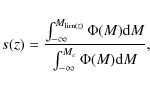 |
(1) |
where
We applied this algorithm to data from the GOODS-MUSIC catalogue, in
a redshift range from ![]() to
to ![]() ,
where we have
sufficient statistics. We performed this analysis by
selecting galaxies brighter than MB=-18 up to redshift 1.8 and
brighter than MB=-19 at higher redshift, to minimise the
completeness correction described above, keeping the average
weight w(z) below 1.6 in all cases.
,
where we have
sufficient statistics. We performed this analysis by
selecting galaxies brighter than MB=-18 up to redshift 1.8 and
brighter than MB=-19 at higher redshift, to minimise the
completeness correction described above, keeping the average
weight w(z) below 1.6 in all cases.
Using this comoving density estimate we analysed the field in two
complementary ways. First, we detected and studied galaxy
overdensities, i.e. clusters or groups (see Sect. 5), defined as
connected 3-dimensional regions with density exceeding a fixed
threshold and a minimum number of members chosen according to the results of the simulations (Sect.
4). In particular, we isolated the structures as the regions having
![]() on our density maps and at least 5 members. We then considered as
part of each structure the spatially connected region (in RA,
Dec, and redshift) around each peak, with an environmental density
of >
on our density maps and at least 5 members. We then considered as
part of each structure the spatially connected region (in RA,
Dec, and redshift) around each peak, with an environmental density
of >![]() above the average and at least 15 member galaxies. To avoid spurious connections
between different structures at the same redshift, we considered
regions within an Abell radius from the peak. The galaxies located
in this region are associated with each structure. We then studied the variation of galaxy
properties as a function of environmental density (Sect.
7), associating the comoving density at its position to each galaxy in the sample.
above the average and at least 15 member galaxies. To avoid spurious connections
between different structures at the same redshift, we considered
regions within an Abell radius from the peak. The galaxies located
in this region are associated with each structure. We then studied the variation of galaxy
properties as a function of environmental density (Sect.
7), associating the comoving density at its position to each galaxy in the sample.
3.1 Comparison with other methods based on photometric redshifts
As mentioned in the introduction, other methods based on photometric redshifts have been developed for the detection of cosmic structures. Here we present the main differences between our algorithm and those that appeared most recently in the literature. However, a more detailed comparison is beyond the scope of the present work, since it would require extensive simulations and/or the application of the different methods to the same datasets.
A similar three-dimensional approach has been proposed by Zatloukal et al. (2007). They select cluster candidates detecting excess density in the 3D galaxy distribution reconstructed from the photometric redshift probability distributions p(z) of each object. However, at variance with our method, they do not adopt any redshift-dependent correction for their estimated density, since they analyse only a narrow redshift range. As we outlined in the previous section, such correction is needed to provide a redshift independent density scale in a deep sample such as the GOODS-MUSIC.
Botzler et al. (2004) expanded the well-known friends-of-friends (FoF)
algorithm (Huchra & Geller 1982), to take photometric redshift uncertainties into account.
This method links groups of individual galaxies if their
redshift difference and angular distances are below fixed
thresholds. These thresholds depend on the photometric redshift
uncertainties, which are greater than the average physical distance
between galaxies and also greater than the velocity dispersion of
rich clusters. This could induce the problem of structures
percolating through excessively large volumes. They dealt with this
issue dividing the catalogue in redshift slices. Instead of
comparing the distance between galaxy pairs, as done in an FoF
approach, we used the statistical information of how many galaxies
are in the neighbourhood of a given point to estimate a physical
density. This approach can avoid the percolation
problem more effectively, since it identifies structures from the 4![]() density peaks
whose extension is limited by the fixed threshold in density.
density peaks
whose extension is limited by the fixed threshold in density.
Several authors, e.g. Scoville et al. (2007), Mazure et al. (2007), Eisenhardt et al. (2008), and van Breukelen et al. (2006) have estimated the surface density in redshift slices, each with different methods: the first two use adaptive smoothing of galaxy counts, Eisenhardt et al. (2008) analyse a density map convolved with a wavelet kernel, while the last author adopts FoF and Voronoi tessellation (Marinoni et al. 2002). At variance with these, we preferred to adopt an adaptive 3D density estimate to consider, automatically, distances in all directions and the relevant positional accuracies at the same time. This approach requires longer computational times, but allows for an increased resolution in high-density regions where the chosen number of objects is found in a smaller volume with respect to field and void regions. As a consequence it also avoids all peculiar ``border'' effects given by the limits of the redshift slices, and there is also no need to adopt additional criteria to decide whether an overdensity, present in two contiguous 2D density maps in similar angular positions, represents the same group or not (as done for example by Mazure et al. 2007). This clearly also depends on the ability of the algorithm to separate aligned structures (for a more detailed discussion of this see Sect. 4).
Finally, another important difference with respect to previous
methods is in the way we use the photometric redshift: some authors
use best-fit values of photometric redshift, e.g. Mazure et al. (2007),
while Scoville et al. (2007), van Breukelen et al. (2006), Zatloukal et al. (2007), and
Eisenhardt et al. (2008) consider the full probability
distribution function (PDF) to take redshift
uncertainties into account. As discussed by Scoville et al. (2007), this last method
could tend to detect structures formed by early type
galaxies, since they have smaller photometric redshift uncertainty, thanks
to their stronger Balmer break, when this feature is well-sampled in
the observed bands. We are less biased in this respect, since we considered the photometric
redshift uncertainty in a conservative way, choosing only the
maximum redshift range where we count neighbour galaxies to associate
with each cell. We took this range as
![]() around
the redshift of each cell, where
around
the redshift of each cell, where
![]() (Grazian et al. 2006a) is the average accuracy of the photometric
redshift in the range we analyse.
(Grazian et al. 2006a) is the average accuracy of the photometric
redshift in the range we analyse.
4 Simulations
We estimated the reliability of our cluster detection algorithm by
testing it on a series of mock catalogues designed to reproduce the
characteristics of the GOODS survey. These mock catalogues are
composed by a given number of groups and clusters superimposed on a
random (Poissonian) field. While this is a rather simplistic
representation of a survey, it allows us to evaluate some basic
features of our algorithm, without the use of N-body simulations. We
expanded the previous simulations presented in Trevese et al. (2007),
using a larger number of mock catalogues and adopting a more
consistent treatment of the survey completeness.
For each redshift, we calculated the limiting absolute B magnitude for the two populations of
``red'' and ``blue'' galaxies, defined from the minima in the U-V vs. B distribution in Salimbeni et al. (2008), using the average type-dependent K- and
evolutionary corrections calculated from the best-fit SED of the
objects in the real catalogue. We then generated an ``observed''
mock catalogue of field galaxies randomly distributed over an area equal to that of the GOODS-South survey. At each redshift, the number of objects in the catalogue is obtained from the
integral of the rest frame B band luminosity function
![]() derived in Salimbeni et al. (2008), up to the limiting absolute MB(z) magnitude computed as described above.
derived in Salimbeni et al. (2008), up to the limiting absolute MB(z) magnitude computed as described above.
Finally, we created different mock catalogues superimposing a number
of structures on the random fields. Given the relatively small
comoving volume sampled by the survey, we expect to find only
groups and small clusters with a total mass
![]() -
-
![]() and a number of members corresponding
to the lowest Abell richness classes (Girardi et al. 1998a). To check that
the performance of the algorithm does not change appreciably with a
varying number of real overdensities of this kind, we performed three different
subset of simulations. Each subset is based on the analysis of 10 mock catalogues, with a number of
groups equal to the number of
and a number of members corresponding
to the lowest Abell richness classes (Girardi et al. 1998a). To check that
the performance of the algorithm does not change appreciably with a
varying number of real overdensities of this kind, we performed three different
subset of simulations. Each subset is based on the analysis of 10 mock catalogues, with a number of
groups equal to the number of
![]() ,
,
![]() ,
and
,
and
![]() DM haloes,
obtained by integrating the Press
DM haloes,
obtained by integrating the Press ![]() Schechter function
(Press & Schechter 1974) over the comoving volume sampled by the survey.
Their positions in real space are chosen randomly. Cluster galaxies
follow a King-like spatial distribution
Schechter function
(Press & Schechter 1974) over the comoving volume sampled by the survey.
Their positions in real space are chosen randomly. Cluster galaxies
follow a King-like spatial distribution
![]() (see Sarazin 1988) with a typical core
radius
(see Sarazin 1988) with a typical core
radius
![]() Mpc.
Mpc.
To consider the uncertainty on photometric redshifts, to each cluster we
assigned galaxy a random redshift extracted from a
Gaussian distribution centred on the cluster redshift
![]() and
having a dispersion
and
having a dispersion
![]() .
We neglected the
cluster real velocity dispersion, which is much smaller than the
.
We neglected the
cluster real velocity dispersion, which is much smaller than the
![]() uncertainty. We analysed the simulations in the same way
as the real catalogue, i.e. calculating galaxy volume density
considering objects with
uncertainty. We analysed the simulations in the same way
as the real catalogue, i.e. calculating galaxy volume density
considering objects with
![]() at z< 1.8 and objects with
at z< 1.8 and objects with
![]() at
at
![]() .
.
We have evaluated the completeness of the sample of detected clusters (fraction of real clusters detected) and its purity (fraction of detected structures corresponding to real ones) at different redshifts (see Table 1). We also present the number of unresolved pairs (a detected structure corresponding to two real ones) and the number of double identifications (a unique real structure separated into two detected ones).
Table 2: Average distances of detected peaks from real centres.
Our aim is to study the properties of individual structures and not, for example, to perform group number counts for
cosmological purposes. For this reason, we prefered to choose conservative selection
criteria in order to maximise the purity of our sample, while still
keeping the completeness high. We isolated the structures as described in Sect. 3, and we considered as significant only those overdensities with at least 5 members in the ![]() region and 15 members in the
region and 15 members in the ![]() region.
region.
A structure in the input catalogue is identified if its centre is within
![]() Mpc projected
distance, and within
Mpc projected
distance, and within
![]() ,
from the centre of a detected
structure, for the low-redshift sample and
,
from the centre of a detected
structure, for the low-redshift sample and
![]() Mpc,
Mpc,
![]() at high z (to account for the increased uncertainties in
redshift and position). The results are reported in Table 1. We can see that the chosen thresholds and
selection criteria allow for a high purity (
at high z (to account for the increased uncertainties in
redshift and position). The results are reported in Table 1. We can see that the chosen thresholds and
selection criteria allow for a high purity (![]()
![]() )
at z <1.8, still detecting about the 80% of the
real structures. At z >1.8, given the greatly
reduced fraction of observed galaxies, the noise is higher, and these
criteria turn out to be very conservative (therefore the
completeness is low) but are necessary to keep a low number
of false detections (purity
)
at z <1.8, still detecting about the 80% of the
real structures. At z >1.8, given the greatly
reduced fraction of observed galaxies, the noise is higher, and these
criteria turn out to be very conservative (therefore the
completeness is low) but are necessary to keep a low number
of false detections (purity ![]() -
-![]() ). Table 2 shows the average distance between the
centres of the real structures and the centres of their detected
counterparts. The density peaks allow the positions of real groups to be identified with
good accuracy.
). Table 2 shows the average distance between the
centres of the real structures and the centres of their detected
counterparts. The density peaks allow the positions of real groups to be identified with
good accuracy.
We also evaluated the ability of the algorithm to separate real
structures that are very close both in redshift and angular
position. In Table 3 we present, for different
intracluster distances, the density level at which couples of real
groups appear as separated peaks. Both at low and high redshift it
is not possible to separate structures whose centres are closer than
1.0 Mpc on the plane of the sky and 2![]() in redshift. For
larger separations, it is possible to separate the groups using higher thresholds (5 or 6
in redshift. For
larger separations, it is possible to separate the groups using higher thresholds (5 or 6 ![]() above
the average
above
the average ![]() ).
).
5 A catalogue of the detected overdensities in the GOODS-South field
Table 3: Separation threshold for aligned groups.
![\begin{figure}
\par\includegraphics[width=8.8cm,clip]{1570fig1.ps}
\end{figure}](/articles/aa/full_html/2009/27/aa11570-08/img94.png) |
Figure 1: Upper panel: photometric redshift distribution of our sample (continuous line). Vertical lines mark the redshifts of the detected structures. Lower panel: redshift distribution of spectroscopically selected AGNs in the GOODS-South field (continuous line); the dashed-line histogram is the distribution of the AGNs associated with the overdensity peaks in Table 4. |
| Open with DEXTER | |
An inspection of the 3-D density map shows some complex high-density structures distributed over the entire GOODS field. In
particular, we found diffuse overdensities at ![]() ,
at
,
at
![]() ,
at
,
at ![]() ,
and at
,
and at ![]() .
Some of these have
already been partially described
(Gilli et al. 2003; Adami et al. 2005; Vanzella et al. 2005; Castellano et al. 2007; Trevese et al. 2007; Díaz-Sánchez et al. 2007). Figure 1 shows the position of these overdensities over the photometric redshift distributions of our sample.These overdensities are also traced by the distribution of the spectroscopically confirmed AGNs in our catalogue, as shown in the lower panel of Fig. 1. (These objects are not included in the sample used for the density estimation.) This link between large-scale structures and AGN distribution was already noted, at lower redshift, in the CDFS
(Gilli et al. 2003), in the E-CDFS (Silverman et al. 2008) and in the CDFN (Barger et al. 2003).
.
Some of these have
already been partially described
(Gilli et al. 2003; Adami et al. 2005; Vanzella et al. 2005; Castellano et al. 2007; Trevese et al. 2007; Díaz-Sánchez et al. 2007). Figure 1 shows the position of these overdensities over the photometric redshift distributions of our sample.These overdensities are also traced by the distribution of the spectroscopically confirmed AGNs in our catalogue, as shown in the lower panel of Fig. 1. (These objects are not included in the sample used for the density estimation.) This link between large-scale structures and AGN distribution was already noted, at lower redshift, in the CDFS
(Gilli et al. 2003), in the E-CDFS (Silverman et al. 2008) and in the CDFN (Barger et al. 2003).
![\begin{figure}
\par\includegraphics[width=17cm,clip]{1570fig2.ps}
\end{figure}](/articles/aa/full_html/2009/27/aa11570-08/img95.png) |
Figure 2:
Density isosurfaces for structures at |
| Open with DEXTER | |
Within these large-scale overdensities, we identified the
structures with the procedure described in Sect. 4.
Using an analysis with a ![]() threshold, we found that two structures identified with
threshold, we found that two structures identified with
![]() ,
at
,
at
![]() ,
and
,
and ![]() ,
are the sum of two different structures, so
we used a
,
are the sum of two different structures, so
we used a ![]() threshold to separate these peaks. We then
associated the galaxies belonging to the region of overlap between the two structures to the
less distant peak.
threshold to separate these peaks. We then
associated the galaxies belonging to the region of overlap between the two structures to the
less distant peak.
Overall, we found four structures at ![]() ,
four structures at
,
four structures at ![]() ,
one at
,
one at
![]() (see also
C07) and three structures at
(see also
C07) and three structures at ![]() .
The density isosurfaces of the structures at
.
The density isosurfaces of the structures at ![]() ,
at
,
at
![]() ,
,
![]() ,
and at
,
and at ![]() are shown in Fig. 2,
superimposed on the ACS z850 band image of the GOODS-South. The analogous image for the overdensity at
are shown in Fig. 2,
superimposed on the ACS z850 band image of the GOODS-South. The analogous image for the overdensity at ![]() is showen in Castellano et al. (2007). In the figure, we indicate the peak position of the identified structures. Other overdensities present did not pass our selection criteria described in Sect. 4.
is showen in Castellano et al. (2007). In the figure, we indicate the peak position of the identified structures. Other overdensities present did not pass our selection criteria described in Sect. 4.
All the structures are presented in Table 4, where we list the following properties:
- Column 1: ID number.
- Columns 2-4: the position of the density peak (redshift, RA, and Dec)
obtained with our 3-D photometric analysis.
- Column 5: the number of the objects associated with each structure
as defined above. This number gives a hint on the richness of the
structure; however, it should not be used to compare structures
at different
redshifts because of the different magnitude intervals sampled.
- Column 6: the average number of field objects present in a volume
equal to that associated to the structure, at the relevant redshift. We
calculated this number by integrating the evolutive LFs obtained by
Salimbeni et al. (2008). In particular, we integrated the LF up to an
absolute limiting magnitude calculated using the average K - and
evolutionary corrections - and z850 limiting observed magnitude
as done in Sect. 4. In this way we take
the selection effects into account given by the magnitude cut in our catalogue,
as a function of redshift.
- Columns 7, 8: the M200 and r200 (assuming bias factors 1
and 2). The mass M200 is defined as the mass inside the radius
corresponding to a density contrast

 200 (Carlberg et al. 1997), where b is the bias factor. To estimate the 3D galaxy density
contrast
200 (Carlberg et al. 1997), where b is the bias factor. To estimate the 3D galaxy density
contrast
 ,
we count the objects in the photometric
redshift range occupied by the structure as a function of the
cluster-centric radius. We then perform a statistical subtraction
of the background/foreground field galaxies, using an area at least
2.5 Mpc (comoving) away from the centre of every cluster in the
relevant redshift interval. Finally, the density contrast is
computed assuming spherical symmetry of the structure.
The mass inside a volume V of density contrast
is
determined by adapting to our case the method used for spectroscopic
data at higher z by Steidel et al. (1998):
,
we count the objects in the photometric
redshift range occupied by the structure as a function of the
cluster-centric radius. We then perform a statistical subtraction
of the background/foreground field galaxies, using an area at least
2.5 Mpc (comoving) away from the centre of every cluster in the
relevant redshift interval. Finally, the density contrast is
computed assuming spherical symmetry of the structure.
The mass inside a volume V of density contrast
is
determined by adapting to our case the method used for spectroscopic
data at higher z by Steidel et al. (1998):
in which is the average density of the Universe and
 is the total mass density contrast related to the galaxy number density contrast through a bias factor:
 .
We assume a
bias factor b in the range
.
We assume a
bias factor b in the range
 (see Arnouts et al. 1999).
- Column 9: the level of the density peak, measured in
number of
 above the average volume density.
In Table 5 we present a value for the X-ray count rate in the band 0.3-4 kev,
the corresponding flux (in the interval 0.5-2 keV) and the
rest-frame luminosity (0.1-2.4 keV), from the Chandra 2Ms exposure
(Luo et al. 2008). We measured the count rates in a square of
side of ![]()
![]() ,
centred on the position of the peak of
each structure. For the count-rate to flux conversion we assumed as spectrum a Raymond-Smith model (Raymond & Smith 1977) with T = 1 keV and 3 keV and metallicity of 0.2
,
centred on the position of the peak of
each structure. For the count-rate to flux conversion we assumed as spectrum a Raymond-Smith model (Raymond & Smith 1977) with T = 1 keV and 3 keV and metallicity of 0.2 ![]() .
.
Table 4: Overdensities in the GOODS-South field.
Table 5: X-ray observations.
5.1 Structures at z
0.7
At redshift
![]() we isolated three high density
peaks (ID = 1, 2 and 3) that are part of a large scale structure
already noted, as a whole, by Gilli et al. (2003).
we isolated three high density
peaks (ID = 1, 2 and 3) that are part of a large scale structure
already noted, as a whole, by Gilli et al. (2003).
For the structure with ID = 1, we estimated the redshift from the
available 6 spectroscopic data. We found an average redshift of
![]() and a velocity dispersion of
and a velocity dispersion of
![]() .
Assuming that the cluster is virialised, we estimated
.
Assuming that the cluster is virialised, we estimated
![]() Mpc and
Mpc and
![]() ,
using
the relations in Girardi et al. (1998b). This estimate is also based
on the assumption that there
are no infalling galaxies and that the surface term (e.g.
Carlberg et al. 1996) is negligible. Considering the uncertainties, also
due to the small number of spectroscopic galaxies,
,
using
the relations in Girardi et al. (1998b). This estimate is also based
on the assumption that there
are no infalling galaxies and that the surface term (e.g.
Carlberg et al. 1996) is negligible. Considering the uncertainties, also
due to the small number of spectroscopic galaxies,
![]() is
fairly consistent with the M200 estimated from the galaxy
density contrast (0.9-
is
fairly consistent with the M200 estimated from the galaxy
density contrast (0.9-
![]() ).
).
We also derived the upper limits on the X-ray luminosities for this
structure, which is close to 0.2-
![]() .
All the properties presented are
consistent with the structure being a galaxy group/small cluster
(Bahcall 1999).
.
All the properties presented are
consistent with the structure being a galaxy group/small cluster
(Bahcall 1999).
The structures with ID = 2, 3 have upper limits on their X-ray
luminosities of the order of 0.2-
![]() ,
and their masses
,
and their masses
![]() -
-
![]() .
These X-ray luminosities and masses are all
typical of galaxy groups/small clusters (Bahcall 1999). Each of these structures contains a spectroscopically confirmed galaxy detected in the VLA 1.4 GHz survey (Miller et al. 2008).
.
These X-ray luminosities and masses are all
typical of galaxy groups/small clusters (Bahcall 1999). Each of these structures contains a spectroscopically confirmed galaxy detected in the VLA 1.4 GHz survey (Miller et al. 2008).
At a slightly higher redshift (![]() ), we identified a
high density peak (ID = 4) embedded in another large-scale
structure that was already known in the literature
(Gilli et al. 2003; Adami et al. 2005; Trevese et al. 2007). In our previous paper
(Trevese et al. 2007), we identified this structure applying our
algorithm to the data from the K20 catalogue, and classified it as
an Abell 0 cluster.
), we identified a
high density peak (ID = 4) embedded in another large-scale
structure that was already known in the literature
(Gilli et al. 2003; Adami et al. 2005; Trevese et al. 2007). In our previous paper
(Trevese et al. 2007), we identified this structure applying our
algorithm to the data from the K20 catalogue, and classified it as
an Abell 0 cluster.
In this new analysis we found that this
structure is symmetric and has a regular mass profile. It has 92 associated objects (
MB(AB)<-18)
and two AGNs. From the density contrast we obtained an
r200=1.7-2.4 Mpc and a total mass of
M200=0.9-
![]() for bias factor b=2-1. From the 36 galaxies with spectroscopic redshifts, we estimated a redshift location of
for bias factor b=2-1. From the 36 galaxies with spectroscopic redshifts, we estimated a redshift location of
![]() and a velocity dispersion of
and a velocity dispersion of
![]() .
We derived a virial radius
.
We derived a virial radius
![]() Mpc, and a virial
mass
Mpc, and a virial
mass
![]() ,
in good agreement
with M200. The 3 sigma upper limit for the X-ray luminosity in
the interval 0.1-2.4 keV is very low (
,
in good agreement
with M200. The 3 sigma upper limit for the X-ray luminosity in
the interval 0.1-2.4 keV is very low (
![]() -
-
![]() ). The area we considered does not include
the X-ray source 173 of Luo et al. (2008), which like
Gilli et al. (2003), we associated to the halo of the brightest cluster
galaxy (ID
). The area we considered does not include
the X-ray source 173 of Luo et al. (2008), which like
Gilli et al. (2003), we associated to the halo of the brightest cluster
galaxy (ID
![]() ). Alternatively, Adami et al. (2005)
associate the bolometric luminosity (
). Alternatively, Adami et al. (2005)
associate the bolometric luminosity (
![]() )
of the X-ray source 173 to the thermal emission of the
intra-cluster medium (ICM). From this value they deduce a galaxy
velocity dispersion around 200-
)
of the X-ray source 173 to the thermal emission of the
intra-cluster medium (ICM). From this value they deduce a galaxy
velocity dispersion around 200-
![]() .
This value
apparently contrasts with the
.
This value
apparently contrasts with the ![]() estimated from the
spectroscopic redshifts. We also associated the object 236 detected in the VLA 1.4 GHz survey to the galaxy ID
estimated from the
spectroscopic redshifts. We also associated the object 236 detected in the VLA 1.4 GHz survey to the galaxy ID
![]() .
It has an integrated emission of
.
It has an integrated emission of
![]() Jy (Miller et al. 2008).
Jy (Miller et al. 2008).
From this analysis we can conclude that our two independent mass
estimates (M200 and
![]() )
are consistent with this
structure being a virialised poor cluster. However, the X-ray
emission is significantly lower than what is expected from its
optical properties, as is shown from the comparison in Fig. 3 with the
)
are consistent with this
structure being a virialised poor cluster. However, the X-ray
emission is significantly lower than what is expected from its
optical properties, as is shown from the comparison in Fig. 3 with the
![]() relations found by Reiprich & Böhringer (2002) and by Rykoff et al. (2008).
relations found by Reiprich & Böhringer (2002) and by Rykoff et al. (2008).
![\begin{figure}
\par\includegraphics[width=8.8cm,clip]{1570fig3.ps}
\end{figure}](/articles/aa/full_html/2009/27/aa11570-08/img148.png) |
Figure 3:
|
| Open with DEXTER | |
5.2 Structures at z
1
At redshift ![]() 1 we found four structures (ID = 5, 6, 7, and 8).
1 we found four structures (ID = 5, 6, 7, and 8).
The structure with ID = 5 at
![]() has 32 member
galaxies. This structure can be associated to the
extended X-ray source number 183 in the catalogue by
Luo et al. (2008) derived from the 2MS Chandra observation. This extended
X-ray source had not been associated to any structure so far. From the count rate
in the interval 0.3-4 keV (
S/N = 11.3) we estimated a luminosity
has 32 member
galaxies. This structure can be associated to the
extended X-ray source number 183 in the catalogue by
Luo et al. (2008) derived from the 2MS Chandra observation. This extended
X-ray source had not been associated to any structure so far. From the count rate
in the interval 0.3-4 keV (
S/N = 11.3) we estimated a luminosity
![]() -
-
![]() (in the interval 0.1-2.4 keV).
For the structures with ID = 6, 7 we estimated
(in the interval 0.1-2.4 keV).
For the structures with ID = 6, 7 we estimated
![]() -1.8 Mpc and a total mass of
M200=0.4-
-1.8 Mpc and a total mass of
M200=0.4-
![]() .
The 3 sigma upper limits for their X-ray luminosity are
all slightly below
.
The 3 sigma upper limits for their X-ray luminosity are
all slightly below
![]() ,
consistent with their M200 masses.
,
consistent with their M200 masses.
The structure with ID = 8 at
![]() has 38 associated galaxies
and an AGN spectroscopically confirmed. We derived a precise
redshift location of
has 38 associated galaxies
and an AGN spectroscopically confirmed. We derived a precise
redshift location of
![]() and a velocity dispersion of
and a velocity dispersion of
![]() ,
from 6 galaxies with spectroscopic
redshift. From these galaxies we also obtained
,
from 6 galaxies with spectroscopic
redshift. From these galaxies we also obtained
![]() and
and
![]() Mpc. We estimated
r200=1.1-1.3 Mpc, and
M200=0.2-
Mpc. We estimated
r200=1.1-1.3 Mpc, and
M200=0.2-
![]() ,
which are compatible values with a group of such
,
which are compatible values with a group of such
![]() and
and
![]() .
This structure was already found with different
methods by Adami et al. (2005), using a FoF algorithm on
spectroscopic data from the VIMOS VLT survey (structure 15 in their
Table 4), and by Díaz-Sánchez et al. (2007) studying the extremely red objects
on GOODS-South. (They call this structure GCL J0332.2-2752.) Their
redshift positions and the velocity dispersions are consistent with
those obtained in the present analysis. The 3 sigma upper limit for
the X-ray luminosity is around
.
This structure was already found with different
methods by Adami et al. (2005), using a FoF algorithm on
spectroscopic data from the VIMOS VLT survey (structure 15 in their
Table 4), and by Díaz-Sánchez et al. (2007) studying the extremely red objects
on GOODS-South. (They call this structure GCL J0332.2-2752.) Their
redshift positions and the velocity dispersions are consistent with
those obtained in the present analysis. The 3 sigma upper limit for
the X-ray luminosity is around
![]() ,
consistent with the estimated M200 mass.
,
consistent with the estimated M200 mass.
Considering their properties, these four structures can be classified as groups of galaxies. Consistent results for the structure with ID = 6 were obtained in Trevese et al. (2007).
5.3 Structures at high z
At redshift
![]() ,
we found a compact structure that corresponds to a forming cluster, as
already discussed in detail by C07 (see also Kurk et al. 2008). We found a
regular mass profile for this structure, and we estimated an
r200=2.1-2.9 Mpc, and a
M200=2.0-
,
we found a compact structure that corresponds to a forming cluster, as
already discussed in detail by C07 (see also Kurk et al. 2008). We found a
regular mass profile for this structure, and we estimated an
r200=2.1-2.9 Mpc, and a
M200=2.0-
![]() .
This structure has 50 members,
including 3 spectroscopic redshifts, and a confirmed AGN from
the GOODS-MUSIC catalogue. We added three other spectroscopic
redshifts from the GMASS sample (Cimatti et al. 2008). From these 6
redshifts we estimated a velocity dispersion of
.
This structure has 50 members,
including 3 spectroscopic redshifts, and a confirmed AGN from
the GOODS-MUSIC catalogue. We added three other spectroscopic
redshifts from the GMASS sample (Cimatti et al. 2008). From these 6
redshifts we estimated a velocity dispersion of
![]() ,
and derived an
,
and derived an
![]() and
and
![]() Mpc. This estimate is consistent with the value in Table 4. We derived an upper limit to the X-ray luminosity of
0.83-
Mpc. This estimate is consistent with the value in Table 4. We derived an upper limit to the X-ray luminosity of
0.83-
![]() (0.1-2.4 KeV), lower than expected from the
velocity dispersion and the estimated M200 (see Fig. 3).
(0.1-2.4 KeV), lower than expected from the
velocity dispersion and the estimated M200 (see Fig. 3).
At ![]() we found a diffuse overdensity, similar to those at
lower redshift, embedding three structures. We associate 20, 23, and 19 galaxies to these
structures.
We estimated an
we found a diffuse overdensity, similar to those at
lower redshift, embedding three structures. We associate 20, 23, and 19 galaxies to these
structures.
We estimated an
![]() -2 Mpc and a mass of
-2 Mpc and a mass of
![]() -
-
![]() for all these structures. These structures appear to be
comparable to those at
for all these structures. These structures appear to be
comparable to those at ![]() 0.7 and
0.7 and ![]() 1.6, and they could be
forming clusters.
1.6, and they could be
forming clusters.
6 Colour-magnitude diagrams
![\begin{figure}
\par\includegraphics[width=8.8cm,clip]{1570fig4.ps}
\end{figure}](/articles/aa/full_html/2009/27/aa11570-08/img165.png) |
Figure 4:
Rest-frame
colour-magnitude relations (U-B vs. MB) for each structure at
|
| Open with DEXTER | |
![\begin{figure}
\par\includegraphics[width=8.8cm,clip]{1570fig5.ps}
\end{figure}](/articles/aa/full_html/2009/27/aa11570-08/img166.png) |
Figure 5:
Same as
Fig. 4. Panel a) structures at |
| Open with DEXTER | |
We studied the colour-magnitude diagrams (U-B vs. MB) for all
the structures, as shown in Figs. 4 and 5. To estimate the slope of the red-sequence, we
defined its members as passively evolving galaxies according to the
physical criterion
![]() ,
where the age and
,
where the age and ![]() (the
star formation e-folding time) we are inferred for each galaxy from the SED fitting (Sect. 2). This quantity is, in practice, the
inverse of the Scalo parameter (Scalo 1986), and a ratio of 4 was chosen to
distinguish galaxies having prevalently evolved stellar populations
from galaxies with recent episodes of star formation. Indeed, an
(the
star formation e-folding time) we are inferred for each galaxy from the SED fitting (Sect. 2). This quantity is, in practice, the
inverse of the Scalo parameter (Scalo 1986), and a ratio of 4 was chosen to
distinguish galaxies having prevalently evolved stellar populations
from galaxies with recent episodes of star formation. Indeed, an
![]() corresponds to a residual 2% of the initial SFR
for an exponential star formation history, as adopted in this paper.
Grazian et al. (2006b) shows that this value can be used to effectively
separate star-forming galaxies from the passively evolving population
(see Grazian et al. 2006b, also for the discussion on the uncertainty associated to this
parameter). Passively evolving galaxies are
indicated in figures as filled squares.
corresponds to a residual 2% of the initial SFR
for an exponential star formation history, as adopted in this paper.
Grazian et al. (2006b) shows that this value can be used to effectively
separate star-forming galaxies from the passively evolving population
(see Grazian et al. 2006b, also for the discussion on the uncertainty associated to this
parameter). Passively evolving galaxies are
indicated in figures as filled squares.
![\begin{figure}
\par\includegraphics[angle=-90,width=16cm,clip]{1570fig6.ps}
\end{figure}](/articles/aa/full_html/2009/27/aa11570-08/img169.png) |
Figure 6: Fraction of red (filled circles) and blue galaxies (filled triangles) at decreasing rest frame B magnitudes ( from top to bottom) in four contiguous intervals of increasing redshift ( from left to right). Vertical error bars indicate the Poissonian uncertainty in each bin. The shaded areas are obtained by smoothing the red (blue) fraction with an adaptive sliding box. The horizontal errorbars indicate the range of density covered by the 5-95% of the total sample. |
| Open with DEXTER | |
Figure 4 shows the colour-magnitude diagrams for
the four structures between z=0.66 and z=0.71. The cluster at
![]() (Panel d) shows a well-defined red sequence, while the
three structures at
(Panel d) shows a well-defined red sequence, while the
three structures at
![]() have fewer passively evolving
galaxies. Therefore, to increase our statistics, we estimated the colour-magnitude slope combining all the four
structures in the interval
0.66<z<0.71 (see Panel a in Fig. 5). We obtained a value
have fewer passively evolving
galaxies. Therefore, to increase our statistics, we estimated the colour-magnitude slope combining all the four
structures in the interval
0.66<z<0.71 (see Panel a in Fig. 5). We obtained a value
![]() for the slope. The resulting colour-magnitude relation is plotted in all
panels in Fig. 4 and in panel a in Fig. 5 as a continuous line. The dotted lines constrain
the error at 1-sigma obtained with a Jackknife analysis. It is possible to see
in Fig. 4 that this average colour-magnitude relation is roughly consistent with the position in the (U-B) vs. B diagram of the galaxies belonging to each single structure. We therefore applied the same method at higher redshift, i.e. we
estimated the slope of the red sequence by combining the different
structures at the same redshift.
for the slope. The resulting colour-magnitude relation is plotted in all
panels in Fig. 4 and in panel a in Fig. 5 as a continuous line. The dotted lines constrain
the error at 1-sigma obtained with a Jackknife analysis. It is possible to see
in Fig. 4 that this average colour-magnitude relation is roughly consistent with the position in the (U-B) vs. B diagram of the galaxies belonging to each single structure. We therefore applied the same method at higher redshift, i.e. we
estimated the slope of the red sequence by combining the different
structures at the same redshift.
Panel b of Fig. 5 shows the colour-magnitude diagram
for the structures at ![]() .
We found a slope of
.
We found a slope of
![]() .
.
Panel c in Fig. 5 shows the colour-magnitude diagram
for the structure at
![]() .
In this case we have galaxies
distributed on less than a magnitude range, which is insufficient to
estimate the slope of the ``red sequence''. However, if we plot the
two sequences obtained at lower redshift, we can see that the few
passively evolving galaxies are consistent with them.
.
In this case we have galaxies
distributed on less than a magnitude range, which is insufficient to
estimate the slope of the ``red sequence''. However, if we plot the
two sequences obtained at lower redshift, we can see that the few
passively evolving galaxies are consistent with them.
Finally, at redshift ![]() 2, we only have 4 passive objects from the combination of 3 structures and there is no evidence of a well-defined red sequence. We note that the colours of these objects are generally bluer than the colour of the relations found at lower redshifts.
2, we only have 4 passive objects from the combination of 3 structures and there is no evidence of a well-defined red sequence. We note that the colours of these objects are generally bluer than the colour of the relations found at lower redshifts.
The values of the slopes of the structures at redshift ![]() 0.7
and
0.7
and ![]() 1 are consistent with those of previous determinations
(e.g. Blakeslee et al. 2003; Trevese et al. 2007; Homeier et al. 2006). We confirm that the observations indicate
no evolution up to redshift
1 are consistent with those of previous determinations
(e.g. Blakeslee et al. 2003; Trevese et al. 2007; Homeier et al. 2006). We confirm that the observations indicate
no evolution up to redshift ![]() 1.
This would imply that the
mass-metallicity relation that produces the red sequence
(Kodama et al. 1998) remains practically constant up to, at least,
1.
This would imply that the
mass-metallicity relation that produces the red sequence
(Kodama et al. 1998) remains practically constant up to, at least, ![]() .
.
7 Galaxy properties as a function of the environment
To each object in the sample we associated the comoving density at its position, and we studied galaxy properties as a continuous function of the environmental density.
7.1 Galaxy populations: bimodality
We studied the variation in the fraction of red and blue galaxies as a function of the environmental density. To separate red and blue galaxies we used the minimum in the bimodal galaxy distribution in the (U-V) vs. B colour-magnitude diagram, derived by Salimbeni et al. (2008). Figure 6 shows the fraction of red and blue galaxies for different rest frame Bmagnitudes in four redshift intervals. In general, for every environment, we found that, at fixed luminosity, the red fraction increases with decreasing redshift, and, at fixed redshift, it increases at increasing B luminosity. We also found that for z<1.2the red fraction increases with density for every luminosity, while this effect is absent at higher redshift.
Our results extend to higher redshift those obtained by
Cucciati et al. (2006) on the VVDS survey, with a shallower spectroscopic
sample that reaches ![]() .
We found that at z>1.2 even
the highest luminosity galaxies are blue, star-forming objects, similar to the results in Cucciati et al. (2006),
although our colour selection is slightly different, since we select two complementary samples in colour, while they select two extreme red and blue populations (
.
We found that at z>1.2 even
the highest luminosity galaxies are blue, star-forming objects, similar to the results in Cucciati et al. (2006),
although our colour selection is slightly different, since we select two complementary samples in colour, while they select two extreme red and blue populations (
![]() and
and
![]() ).
Our results also agree with the analysis of the DEEP2 survey
by Cooper et al. (2007) in the redshift range
0.4<z<1.35. They find
a weak correlation between red fraction and density at
).
Our results also agree with the analysis of the DEEP2 survey
by Cooper et al. (2007) in the redshift range
0.4<z<1.35. They find
a weak correlation between red fraction and density at ![]() .
We see that at z>1.2 this correlation disappears, indicating that
the change probably occurs in the critical range 1.5<z<2.0, at
least in the environments probed by our sample. However, we note
that, given the relatively small area covered, we do not probe very
high-density regions (i.e. rich clusters), at variance with wide,
low-redshift surveys. When rich clusters are considered
(e.g. Balogh et al. 2004), a stronger variation with environment in the
colours of faint galaxies is seen. In any case, the disappearance at z>1.2 of the variation in the red fraction in the density range probed by our sample
indicates that a relevant change in
galaxy properties takes place at
.
We see that at z>1.2 this correlation disappears, indicating that
the change probably occurs in the critical range 1.5<z<2.0, at
least in the environments probed by our sample. However, we note
that, given the relatively small area covered, we do not probe very
high-density regions (i.e. rich clusters), at variance with wide,
low-redshift surveys. When rich clusters are considered
(e.g. Balogh et al. 2004), a stronger variation with environment in the
colours of faint galaxies is seen. In any case, the disappearance at z>1.2 of the variation in the red fraction in the density range probed by our sample
indicates that a relevant change in
galaxy properties takes place at ![]() -2.
-2.
7.2 Galaxy physical properties in high and low density environments
![\begin{figure}
\par\includegraphics[width=9cm,clip]{1570fig7.ps}
\end{figure}](/articles/aa/full_html/2009/27/aa11570-08/img181.png) |
Figure 7:
Galaxy
stellar mass distribution in four redshift intervals. Shaded red
histograms represent galaxies associated with the density peaks and
empty black histograms represent galaxies in the low-density regions, as
described in the text. In each panel the average value of |
| Open with DEXTER | |
![\begin{figure}
\par\includegraphics[width=9cm,clip]{1570fig8.ps}
\end{figure}](/articles/aa/full_html/2009/27/aa11570-08/img183.png) |
Figure 8:
Top: as in Fig.
7 but for the ages of galaxies. The average value of the age for the two
distributions are indicated by arrows. Bottom: as in Fig.
7 but for SFR of galaxies. The average values of the
|
| Open with DEXTER | |
We then studied the distribution of physical parameters and photometric
properties for galaxies in high-density environments, and
compare it to field galaxies. The first sample is
defined as the combination of the data from structures with similar
redshifts (``group galaxies'' hereafter). The field galaxies are
defined as those with an associated ![]() lower than the median
density (0.0126 for z<1.8 and 0.0085 for z>1.8) of the entire sample (``field galaxies'' hereafter). We
quantified the differences in the distributions of the galaxy physical properties, i.e. mass, age, star formation rate, through the
probability
lower than the median
density (0.0126 for z<1.8 and 0.0085 for z>1.8) of the entire sample (``field galaxies'' hereafter). We
quantified the differences in the distributions of the galaxy physical properties, i.e. mass, age, star formation rate, through the
probability
![]() of the two samples, obtained as described above, using a Kolmgorov-Smirnov test. We rejected the
hypothesis that two samples are drawn from the same distribution if
of the two samples, obtained as described above, using a Kolmgorov-Smirnov test. We rejected the
hypothesis that two samples are drawn from the same distribution if
![]() .
.
Figure 7 shows the distribution of the galaxy total
stellar mass in high and low density regions, in the same four
contiguous redshift intervals used before. The galaxies in a high-density
environment have a distribution that generally peaks at higher
masses with respect to ``field'' galaxies. For the mass distribution, we found a significant
difference in all but the last redshift bin as shown from the
![]() .
It is important to
point out here that the shape of the distributions at low masses could
depend on the luminosity selection. In fact, a magnitude-limited
sample does not have a well-defined limit in stellar mass. This
effect depends on the range of M/L ratio spanned by galaxies with
different colours, e. g. as shown in Fontana et al. (2006) in our sample, at
.
It is important to
point out here that the shape of the distributions at low masses could
depend on the luminosity selection. In fact, a magnitude-limited
sample does not have a well-defined limit in stellar mass. This
effect depends on the range of M/L ratio spanned by galaxies with
different colours, e. g. as shown in Fontana et al. (2006) in our sample, at ![]() ,
M/LKextends from 0.9, for redder objects, to 0.046, for bluer objects. If a colour segregation is present as a function
of the environment, it could bias the distribution favouring the
observation of lower mass galaxies in less dense regions, where
the fraction of blue galaxies is higher. Although, as shown in Fig.
6, we did not find strong colour
segregation, especially at z>1, we also carried out a more conservative analysis here.
We considered only the range of masses above the completeness mass limit obtained from the maximal
M/Lz850 for a passively evolving system (
,
M/LKextends from 0.9, for redder objects, to 0.046, for bluer objects. If a colour segregation is present as a function
of the environment, it could bias the distribution favouring the
observation of lower mass galaxies in less dense regions, where
the fraction of blue galaxies is higher. Although, as shown in Fig.
6, we did not find strong colour
segregation, especially at z>1, we also carried out a more conservative analysis here.
We considered only the range of masses above the completeness mass limit obtained from the maximal
M/Lz850 for a passively evolving system (
![]() at
at
![]() ,
,
![]() at
at ![]() ,
,
![]() at
at
![]() ,
and
,
and
![]() at
at
![]() ). Considering
galaxies above these mass limits we found that the masses of ``group''
galaxies are still higher than those of ``field'' galaxies for the lower bin in redshift (
). Considering
galaxies above these mass limits we found that the masses of ``group''
galaxies are still higher than those of ``field'' galaxies for the lower bin in redshift (
![]() ). At z > 1.2, however, it is not possible to give a conclusive result
because of the low statistic caused by this mass cut.
). At z > 1.2, however, it is not possible to give a conclusive result
because of the low statistic caused by this mass cut.
Analogous results are found from the analysis of the luminosity distribution of ``field'' and ``group'' galaxies. In particular, we found that the distribution of galaxies in ``groups'' have on average brighter MIrest-frame magnitudes at all redshifts. The results are also similar for the other rest frame bands, implying that galaxies in high-density environments have, on average, greater bolometric luminosity than do field galaxies.
Finally, we studied the age and SFR distributions for ``group'' and ``field''
galaxies (see Fig. 8). Only at low redshift does there appear to be a significant
difference (respectively
![]() and
and
![]() ,
see Fig. 8). The
two age distributions show a similar shape for young galaxies, but
``group'' galaxies have a higher fraction of old galaxies. As also
shown by the difference in the average ages for the two samples, the
``group'' galaxies are older than the field ones. At higher redshifts,
the two distributions do not show any significative differences. Indeed,
at higher redshifts, any possible difference in the age of the
two galaxy populations is probably less than the uncertainty on the
ages. Analogously, star-forming galaxies have a similar distribution for ``group'' and ``field'' samples, but the ``group'' sample has a higher faction of galaxies with low star formation as also shown by the different values of the average SFR.
,
see Fig. 8). The
two age distributions show a similar shape for young galaxies, but
``group'' galaxies have a higher fraction of old galaxies. As also
shown by the difference in the average ages for the two samples, the
``group'' galaxies are older than the field ones. At higher redshifts,
the two distributions do not show any significative differences. Indeed,
at higher redshifts, any possible difference in the age of the
two galaxy populations is probably less than the uncertainty on the
ages. Analogously, star-forming galaxies have a similar distribution for ``group'' and ``field'' samples, but the ``group'' sample has a higher faction of galaxies with low star formation as also shown by the different values of the average SFR.
8 Summary and conclusions
We applied a (2+1)D algorithm on the GOODS-MUSIC catalogue to
identify structures in this area. This algorithm combines galaxy
angular positions and precise photometric redshifts to give an
adaptive estimate of the 3D density field effectively also at z>1and in a wide area. In this way we obtained a density map from
redshift 0.4 up to 2.5, and we isolated the higher density regions.
To identify density peaks we chose a conservative selection criterion (at least five galaxies in connected regions of
![]() )
in order to maximise the purity of our
sample.
)
in order to maximise the purity of our
sample.
We built mock catalogues simulating the GOODS-South
field. Applying our density thresholds and selection
criteria to these catalogues, we found a purity near 100% (with less than 15-20% of
lost structures) up to redshift 1.8, and ![]() 75-80% at higher
redshift. In the higher redshift range, the criterion is very
conservative, to keep a low number of false detections, therefore
the completeness is low (<40%). From the simulations we also
evaluated the ability of the algorithm in separating real structures
that are very close both in redshift and angular position. Both at
low and high redshift it is not possible to separate structures
whose centres are closer than 1.0 Mpc on the plane of the sky and
75-80% at higher
redshift. In the higher redshift range, the criterion is very
conservative, to keep a low number of false detections, therefore
the completeness is low (<40%). From the simulations we also
evaluated the ability of the algorithm in separating real structures
that are very close both in redshift and angular position. Both at
low and high redshift it is not possible to separate structures
whose centres are closer than 1.0 Mpc on the plane of the sky and
![]() in redshift. For larger separations it is possible to
distinguish the groups, but by using higher thresholds (5 or 6
in redshift. For larger separations it is possible to
distinguish the groups, but by using higher thresholds (5 or 6![]() above the average).
above the average).
We found large-scale overdensities at different redshifts (![]() 0.6,
0.6, ![]() 1,
1, ![]() 1.61 and
1.61 and ![]() 2.2), which are well
traced by the AGN distribution, suggesting that the environment on
large scales (
2.2), which are well
traced by the AGN distribution, suggesting that the environment on
large scales (![]() 10 Mpc) has an influence on AGN evolution
(Silverman et al. 2008). We
isolated several groups and small clusters embedded in these large-scale structures. Most of the structures
at
10 Mpc) has an influence on AGN evolution
(Silverman et al. 2008). We
isolated several groups and small clusters embedded in these large-scale structures. Most of the structures
at ![]() and
and ![]() 1 have properties of groups of galaxies: their
masses are of the order of
M200= 0.2-
1 have properties of groups of galaxies: their
masses are of the order of
M200= 0.2-
![]() ,
and their X-ray luminosities are slightly below
,
and their X-ray luminosities are slightly below
![]() ,
consistent with the expectations of the M200-
,
consistent with the expectations of the M200-![]() relations. The structure at z=0.71 and those at z>1.6seem to be more massive, and in particular the structures with ID = 4, and 9
can be classified as poor clusters. It is interesting to note that both these
structures are significantly X-ray underluminous, as is evident by a comparison with the M200-
relations. The structure at z=0.71 and those at z>1.6seem to be more massive, and in particular the structures with ID = 4, and 9
can be classified as poor clusters. It is interesting to note that both these
structures are significantly X-ray underluminous, as is evident by a comparison with the M200-![]() relations found by Reiprich & Böhringer (2002) and by Rykoff et al. (2008, Fig. 3). This is
not surprising since several authors have observed that optically
selected structures have an X-ray emission lower than what is
expected from the observations of X-ray selected groups and
clusters. This effect has been observed at low redshift in
small groups (Rasmussen et al. 2006), in Abell clusters
(Popesso et al. 2007), and in clusters at 0.6<z<1.1(Lubin et al. 2004). These results may be explained by the
optically selected structures still being in the
process of formation or the result of the alignment of two substructures along the line of sight, although it cannot be excluded that they
contain less intracluster gas than expected, because of the effect
of strong galactic feedback (Rasmussen et al. 2006). If these
structures are virialised, as is probable in the case of the massive structure at z=0.71(ID = 4), this may indicate that they contain less
intracluster gas than expected. It is worth investigating this issue in future
deep surveys, since it would have interesting implications for the
evolution of the baryonic content of these structures.
relations found by Reiprich & Böhringer (2002) and by Rykoff et al. (2008, Fig. 3). This is
not surprising since several authors have observed that optically
selected structures have an X-ray emission lower than what is
expected from the observations of X-ray selected groups and
clusters. This effect has been observed at low redshift in
small groups (Rasmussen et al. 2006), in Abell clusters
(Popesso et al. 2007), and in clusters at 0.6<z<1.1(Lubin et al. 2004). These results may be explained by the
optically selected structures still being in the
process of formation or the result of the alignment of two substructures along the line of sight, although it cannot be excluded that they
contain less intracluster gas than expected, because of the effect
of strong galactic feedback (Rasmussen et al. 2006). If these
structures are virialised, as is probable in the case of the massive structure at z=0.71(ID = 4), this may indicate that they contain less
intracluster gas than expected. It is worth investigating this issue in future
deep surveys, since it would have interesting implications for the
evolution of the baryonic content of these structures.
We then studied the colour magnitude diagrams (U-B vs. MB) for
all the structures. We defined the members of the red sequence
according to the physical criterion
![]() ,
which should
select passively evolving galaxies with little residual star
formation. We confirmed no evolution of the red sequence slope up to
redshift
,
which should
select passively evolving galaxies with little residual star
formation. We confirmed no evolution of the red sequence slope up to
redshift ![]() 1.
This implies that the mass-metallicity relation that produces
the slope of the red sequence remains constant up to
1.
This implies that the mass-metallicity relation that produces
the slope of the red sequence remains constant up to ![]() .
.
We then studied the variation in the fraction of red and blue galaxies as a function of the environmental density. We found that, at fixed redshift, the red fraction increases at increasing B luminosity, while, at fixed luminosity, it increases with decreasing redshift. We found that the increment of the red fraction at growing density disappears at z>1.2.
We also studied galaxy properties in different environments. We found that the galaxies in high-density environments have higher masses with respect to ``field galaxies'', in qualitative agreement with a downsizing scenario. The mass distributions show a significant difference in all but the last redshift bin. Similarly, the galaxies in groups have on average brighter rest-frame magnitudes, and there are a greater number of bright galaxies in groups at all redshifts compared to field galaxies. Finally, the age and SFR distributions for the two subsamples appear different only at low redshifts where ``group galaxies'' are generally older and less star forming than ``field'' ones.
From the analysis of the environmental
dependence of galaxy colours and mass as a function of redshift, and from the absence of any
well-defined red sequence at high redshift, we can argue that
a critical period in which some basic characteristics of galaxy
populations are established is that between ![]() and
and ![]() .
.
Acknowledgements
We thank the anonymous referee for his/her helpful comments. S.S. acknowledges support from the UMASS Department of Astronomy through a postdoctoral fellowship.
References
- Adami, C., Mazure, A., Ilbert, O., et al. 2005, A&A, 443, 805 [NASA ADS] [CrossRef] [EDP Sciences]
- Arnouts, S., Cristiani, S., Moscardini, L., et al. 1999, MNRAS, 310, 540 [NASA ADS] [CrossRef] (In the text)
- Bahcall, N. A. 1999, in Formation of Structure in the Universe, ed. A. Dekel, & J. P. Ostriker, 135 (In the text)
- Balogh, M. L., Baldry, I. K., Nichol, R., et al. 2004, ApJ, 615, L101 [NASA ADS] [CrossRef] (In the text)
- Barger, A. J., Cowie, L. L., Capak, P., et al. 2003, AJ, 126, 632 [NASA ADS] [CrossRef] (In the text)
- Beers, T. C., Flynn, K., & Gebhardt, K. 1990, AJ, 100, 32 [NASA ADS] [CrossRef] (In the text)
- Blakeslee, J. P., Franx, M., Postman, M., et al. 2003, ApJ, 596, L143 [NASA ADS] [CrossRef]
- Blanton, M. R., Eisenstein, D., Hogg, D. W., Schlegel, D. J., & Brinkmann, J. 2005, ApJ, 629, 143 [NASA ADS] [CrossRef]
- Botzler, C. S., Snigula, J., Bender, R., & Hopp, U. 2004, MNRAS, 349, 425 [NASA ADS] [CrossRef]
- Bremer, M. N., Valtchanov, I., Willis, J., et al. 2006, MNRAS, 371, 1427 [NASA ADS] [CrossRef]
- Bruzual, G., & Charlot, S. 2003, MNRAS, 344, 1000 [NASA ADS] [CrossRef] (In the text)
- Carlberg, R. G., Yee, H. K. C., & Ellingson, E. 1997, ApJ, 478, 462 [NASA ADS] [CrossRef] (In the text)
- Carlberg, R. G., Yee, H. K. C., Ellingson, E., et al. 1996, ApJ, 462, 32 [NASA ADS] [CrossRef] (In the text)
- Carlstrom, J. E., Holder, G. P., & Reese, E. D. 2002, ARA&A, 40, 643 [NASA ADS] [CrossRef]
- Castellano, M., Salimbeni, S., Trevese, D., et al. 2007, ApJ, 671, 1497 [NASA ADS] [CrossRef] (In the text)
- Cimatti, A., Mignoli, M., Daddi, E., et al. 2002, A&A, 392, 395 [NASA ADS] [CrossRef] [EDP Sciences] (In the text)
- Cimatti, A., Cassata, P., Pozzetti, L., et al. 2008, A&A, 482, 21 [NASA ADS] [CrossRef] [EDP Sciences] (In the text)
- Cooper, M. C., Newman, J. A., Coil, A. L., et al. 2007, MNRAS, 376, 1445 [NASA ADS] [CrossRef]
- Cucciati, O., Iovino, A., Marinoni, C., et al. 2006, A&A, 458, 39 [NASA ADS] [CrossRef] [EDP Sciences]
- Díaz-Sánchez, A., Villo-Pérez, I., Pérez-Garrido, A., & Rebolo, R. 2007, MNRAS, 377, 516 [NASA ADS] [CrossRef]
- Dressler, A., Oemler, A. J., Couch, W. J., et al. 1997, ApJ, 490, 577 [NASA ADS] [CrossRef]
- Eisenhardt, P. R. M., Brodwin, M., Gonzalez, A. H., et al. 2008, ApJ, 684, 905 [NASA ADS] [CrossRef]
- Elbaz, D., Daddi, E., Le Borgne, D., et al. 2007, A&A, 468, 33 [NASA ADS] [CrossRef] [EDP Sciences]
- Fontana, A., D'Odorico, S., Poli, F., et al. 2000, AJ, 120, 2206 [NASA ADS] [CrossRef] (In the text)
- Fontana, A., Salimbeni, S., Grazian, A., et al. 2006, A&A, 459, 745 [NASA ADS] [CrossRef] [EDP Sciences] (In the text)
- Gilli, R., Cimatti, A., Daddi, E., et al. 2003, ApJ, 592, 721 [NASA ADS] [CrossRef]
- Girardi, M., Borgani, S., Giuricin, G., Mardirossian, F., & Mezzetti, M. 1998a, ApJ, 506, 45 [NASA ADS] [CrossRef] (In the text)
- Girardi, M., Giuricin, G., Mardirossian, F., Mezzetti, M., & Boschin, W. 1998b, ApJ, 505, 74 [NASA ADS] [CrossRef] (In the text)
- Gladders, M. D., & Yee, H. K. C. 2000, AJ, 120, 2148 [NASA ADS] [CrossRef] (In the text)
- Gladders, M. D., & Yee, H. K. C. 2005, ApJS, 157, 1 [NASA ADS] [CrossRef] (In the text)
- Goto, T., Hanami, H., Im, M., et al. 2008, PASJ, 60, 531 [NASA ADS]
- Grazian, A., Fontana, A., de Santis, C., et al. 2006a, A&A, 449, 951 [NASA ADS] [CrossRef] [EDP Sciences] (In the text)
- Grazian, A., Fontana, A., Moscardini, L., et al. 2006b, A&A, 453, 507 [NASA ADS] [CrossRef] [EDP Sciences] (In the text)
- Grazian, A., Salimbeni, S., Pentericci, L., et al. 2007, A&A, 465, 393 [NASA ADS] [CrossRef] [EDP Sciences]
- Homeier, N. L., Mei, S., Blakeslee, J. P., et al. 2006, ApJ, 647, 256 [NASA ADS] [CrossRef]
- Huchra, J. P., & Geller, M. J. 1982, ApJ, 257, 423 [NASA ADS] [CrossRef] (In the text)
- Kodama, T., Arimoto, N., Barger, A. J., & Arag'on-Salamanca, A. 1998, A&A, 334, 99 [NASA ADS] (In the text)
- Kodama, T., Tanaka, I., Kajisawa, M., et al. 2007, MNRAS, 377, 1717 [NASA ADS] [CrossRef]
- Kurk, J., Cimatti, A., Zamorani, G., et al. 2008, in ASP Conf. Ser. 399, ed. T. Kodama, T. Yamada, & K. Aoki, 332 (In the text)
- Le Fèvre, O., Vettolani, G., Paltani, S., et al. 2004, A&A, 428, 1043 [NASA ADS] [CrossRef] [EDP Sciences]
- Lidman, C., Rosati, P., Tanaka, M., et al. 2008, A&A, 489, 981 [NASA ADS] [CrossRef] [EDP Sciences]
- Lubin, L. M., Mulchaey, J. S., & Postman, M. 2004, ApJ, 601, L9 [NASA ADS] [CrossRef]
- Luo, B., Bauer, F. E., Brandt, W. N., et al. 2008, ApJS, 179, 19 [NASA ADS] [CrossRef] (In the text)
- Marinoni, C., Davis, M., Newman, J. A., & Coil, A. L. 2002, ApJ, 580, 122 [NASA ADS] [CrossRef] (In the text)
- Maughan, B. J., Jones, L. R., Ebeling, H., & Scharf, C. 2004, MNRAS, 351, 1193 [NASA ADS] [CrossRef]
- Mazure, A., Adami, C., Pierre, M., et al. 2007, A&A, 467, 49 [NASA ADS] [CrossRef] [EDP Sciences]
- Mei, S., Holden, B. P., Blakeslee, J. P., et al. 2006, ApJ, 644, 759 [NASA ADS] [CrossRef]
- Menci, N., Rosati, P., Gobat, R., et al. 2008, ApJ, 685, 863 [NASA ADS] [CrossRef]
- Mignoli, M., Cimatti, A., Zamorani, G., et al. 2005, A&A, 437, 883 [NASA ADS] [CrossRef] [EDP Sciences]
- Miller, N. A., Fomalont, E. B., Kellermann, K. I., et al. 2008, ApJS, 179, 114 [NASA ADS] [CrossRef] (In the text)
- Nakata, F., Kodama, T., Shimasaku, K., et al. 2005, MNRAS, 357, 1357 [NASA ADS] [CrossRef]
- Popesso, P., Biviano, A., Böhringer, H., & Romaniello, M. 2007, A&A, 461, 397 [NASA ADS] [CrossRef] [EDP Sciences]
- Postman, M., Lubin, L. M., Gunn, J. E., et al. 1996, AJ, 111, 615 [NASA ADS] [CrossRef] (In the text)
- Press, W. H., & Schechter, P. 1974, ApJ, 187, 425 [NASA ADS] [CrossRef] (In the text)
- Rasmussen, J., Ponman, T. J., Mulchaey, J. S., Miles, T. A., & Raychaudhury, S. 2006, MNRAS, 373, 653 [NASA ADS] [CrossRef]
- Raymond, J. C., & Smith, B. W. 1977, ApJS, 35, 419 [NASA ADS] [CrossRef] (In the text)
- Reiprich, T. H., & Böhringer, H. 2002, ApJ, 567, 716 [NASA ADS] [CrossRef] (In the text)
- Rettura, A., Rosati, P., Nonino, M., et al. 2008, ArXiv e-prints
- Rykoff, E. S., Evrard, A. E., McKay, T. A., et al. 2008, MNRAS, 387, L28 [NASA ADS] (In the text)
- Salimbeni, S., Giallongo, E., Menci, N., et al. 2008, A&A, 477, 763 [NASA ADS] [CrossRef] [EDP Sciences] (In the text)
- Sarazin, C. L. 1988, X-ray emission from clusters of galaxies Cambridge Astrophysics Series (Cambridge: Cambridge University Press) (In the text)
- Scalo, J. M. 1986, Fundamentals of Cosmic Physics, 11, 1 [NASA ADS] (In the text)
- Scoville, N., Aussel, H., Benson, A., et al. 2007, ApJS, 172, 150 [NASA ADS] [CrossRef]
- Silverman, J. D., Mainieri, V., Lehmer, B. D., et al. 2008, ApJ, 675, 1025 [NASA ADS] [CrossRef] (In the text)
- Stanford, S. A., Eisenhardt, P. R., Brodwin, M., et al. 2005, ApJ, 634, L129 [NASA ADS] [CrossRef]
- Stanford, S. A., Romer, A. K., Sabirli, K., et al. 2006, ApJ, 646, L13 [NASA ADS] [CrossRef]
- Staniszewski, Z., Ade, P. A. R., Aird, K. A., et al. 2008, ArXiv e-prints
- Steidel, C. C., Adelberger, K. L., Dickinson, M., et al. 1998, ApJ, 492, 428 [NASA ADS] [CrossRef] (In the text)
- Szokoly, G. P., Bergeron, J., Hasinger, G., et al. 2004, ApJS, 155, 271 [NASA ADS] [CrossRef]
- Tran, K.-V. H., van Dokkum, P., Illingworth, G. D., et al. 2005, ApJ, 619, 134 [NASA ADS] [CrossRef]
- Treu, T., Ellis, R. S., Kneib, J.-P., et al. 2003, ApJ, 591, 53 [NASA ADS] [CrossRef]
- Trevese, D., Castellano, M., Fontana, A., & Giallongo, E. 2007, A&A, 463, 853 [NASA ADS] [CrossRef] [EDP Sciences] (In the text)
- van Breukelen, C., Clewley, L., Bonfield, D. G., et al. 2006, MNRAS, 373, L26 [NASA ADS]
- Vanzella, E., Cristiani, S., Dickinson, M., et al. 2005, A&A, 434, 53 [NASA ADS] [CrossRef] [EDP Sciences]
- Vanzella, E., Cristiani, S., Dickinson, M., et al. 2006, A&A, 454, 423 [NASA ADS] [CrossRef] [EDP Sciences]
- Vanzella, E., Cristiani, S., Dickinson, M., et al. 2008, A&A, 478, 83 [NASA ADS] [CrossRef] [EDP Sciences]
- Wolf, C., Meisenheimer, K., Röser, H.-J., et al. 2001, A&A, 365, 681 [NASA ADS] [CrossRef] [EDP Sciences]
- Zatloukal, M., Röser, H.-J., Wolf, C., Hippelein, H., & Falter, S. 2007, A&A, 474, L5 [NASA ADS] [CrossRef] [EDP Sciences]
All Tables
Table 1: Completeness and purity.
Table 2: Average distances of detected peaks from real centres.
Table 3: Separation threshold for aligned groups.
Table 4: Overdensities in the GOODS-South field.
Table 5: X-ray observations.
All Figures
| |
Figure 1: Upper panel: photometric redshift distribution of our sample (continuous line). Vertical lines mark the redshifts of the detected structures. Lower panel: redshift distribution of spectroscopically selected AGNs in the GOODS-South field (continuous line); the dashed-line histogram is the distribution of the AGNs associated with the overdensity peaks in Table 4. |
| Open with DEXTER | |
| In the text | |
| |
Figure 2:
Density isosurfaces for structures at |
| Open with DEXTER | |
| In the text | |
| |
Figure 3:
|
| Open with DEXTER | |
| In the text | |
| |
Figure 4:
Rest-frame
colour-magnitude relations (U-B vs. MB) for each structure at
|
| Open with DEXTER | |
| In the text | |
| |
Figure 5:
Same as
Fig. 4. Panel a) structures at |
| Open with DEXTER | |
| In the text | |
| |
Figure 6: Fraction of red (filled circles) and blue galaxies (filled triangles) at decreasing rest frame B magnitudes ( from top to bottom) in four contiguous intervals of increasing redshift ( from left to right). Vertical error bars indicate the Poissonian uncertainty in each bin. The shaded areas are obtained by smoothing the red (blue) fraction with an adaptive sliding box. The horizontal errorbars indicate the range of density covered by the 5-95% of the total sample. |
| Open with DEXTER | |
| In the text | |
| |
Figure 7:
Galaxy
stellar mass distribution in four redshift intervals. Shaded red
histograms represent galaxies associated with the density peaks and
empty black histograms represent galaxies in the low-density regions, as
described in the text. In each panel the average value of |
| Open with DEXTER | |
| In the text | |
| |
Figure 8:
Top: as in Fig.
7 but for the ages of galaxies. The average value of the age for the two
distributions are indicated by arrows. Bottom: as in Fig.
7 but for SFR of galaxies. The average values of the
|
| Open with DEXTER | |
| In the text | |
Copyright ESO 2009
Current usage metrics show cumulative count of Article Views (full-text article views including HTML views, PDF and ePub downloads, according to the available data) and Abstracts Views on Vision4Press platform.
Data correspond to usage on the plateform after 2015. The current usage metrics is available 48-96 hours after online publication and is updated daily on week days.
Initial download of the metrics may take a while.