The orbital velocity anisotropy of cluster galaxies: evolution

A. Biviano; B. M. Poggianti

doi:10.1051/0004-6361/200911757

Free Access

Issue		A&A Volume 501, Number 2, July II 2009


Page(s)		419 - 427
Section		Cosmology (including clusters of galaxies)
DOI		https://doi.org/10.1051/0004-6361/200911757
Published online		19 May 2009

The orbital velocity anisotropy of cluster galaxies: evolution

A. Biviano¹ - B. M. Poggianti²

1 - INAF/Osservatorio Astronomico di Trieste, via G. B. Tiepolo 11, 34131, Trieste, Italy
2 - INAF/Osservatorio Astronomico di Padova, vicolo Osservatorio 5, 35122, Padova, Italy

Received 30 January 2009 / Accepted 7 May 2009

Abstract
Context. In nearby clusters early-type galaxies follow isotropic orbits. The orbits of late-type galaxies are instead characterized by slightly radial anisotropy. Little is known about the orbits of the different populations of cluster galaxies at redshift z > 0.3.
Aims. We investigate the redshift evolution of the orbits of cluster galaxies.
Methods. We use two samples of galaxy clusters spanning similar (evolutionary corrected) mass ranges at different redshifts. The sample of low-redshift ( $z \sim 0.0{-}0.1$ ) clusters is extracted from the ESO Nearby Abell Cluster Survey (ENACS) catalog. The sample of high-redshift ( $z \sim 0.4{-}0.8$ ) clusters is mostly made of clusters from the ESO Distant Cluster Survey (EDisCS). For each of these samples, we solve the Jeans equation for hydrostatic equilibrium separately for two cluster galaxy populations, characterized by the presence and, respectively, absence of emission-lines in their spectra (``ELGs'' and ``nELGs'' hereafter). Using two tracers of the gravitational potential allows to partially break the mass-anisotropy degeneracy which plagues these kinds of analyses.
Results. We confirm earlier results for the nearby cluster sample. The mass profile is well fitted by a Navarro, Frenk & White (NFW) profile with concentration c=4. The mass profile of the distant cluster sample is also well fitted by a NFW profile, but with a slightly lower concentration, as predicted by cosmological simulations of cluster-sized halos. While the mass density profile becomes less concentrated with redshift, the number density profile of nELGs becomes more concentrated with redshift. In nearby clusters, the velocity anisotropy profile of nELGs is close to isotropic, while that of ELGs is increasingly radial with clustercentric radius. In distant clusters the projected phase-space distributions of both nELGs and ELGs are best-fitted by models with radial velocity anisotropy.
Conclusions. No significant evolution is detected for the orbits of ELGs, while the orbits of nELGs evolve from radial to isotropic with time. We speculate that this evolution may be driven by the secular mass growth of galaxy clusters during their fast accretion phase. Cluster mass density profiles and their evolution with redshift are consistent with predictions for cluster-sized halos in $\Lambda$ Cold Dark Matter cosmological simulations. The evolution of the nELG number density profile is opposite to that of the mass density profile, becoming less concentrated with time, probably a result of the transformation of ELGs into nELGs.

Key words: galaxies: clusters: general - galaxies: evolution - galaxies: kinematics and dynamics

1 Introduction

The distributions of cluster early-type and late-type galaxies (ETGs and LTGs hereafter) have long been known to be different (Dressler 1980; see also Biviano 2000, for a review). Most striking, and hence the first to have been discovered, is the difference in the spatial distributions, ETGs living in higher density regions than LTGs, the so-called ``morphology-density relation'' (MDR hereafter). In relaxed clusters density is an almost monotonic decreasing function of clustercentric radius, hence the relation is often described as a morphology-radius relation (e.g. Whitmore et al. 1993). The MDR has been found to exist in rich clusters up to redshift $z \sim 1$ (Smith et al. 2005; Postman et al. 2005), but the global fractions of ETGs and LTGs evolve with z. The fraction of ETGs in clusters decreases with z quite rapidly up to $z \sim 0.5$ (Smith et al. 2005; Dressler et al. 1997; Postman et al. 2005; Fasano et al. 2000), then seems to flatten out to $z \sim 1$ (Desai et al. 2007).

Another aspect of the segregation of different galaxy populations in clusters is the difference in the velocity distributions of ETGs and LTGs. In clusters, the velocity distribution of LTGs is broader than that of ETGs, i.e. LTGs have a larger line-of-sight (los hereafter) velocity dispersion ( $\sigma _{\rm los}$ hereafter) than ETGs (Tammann 1972; Sodré et al. 1989; Biviano et al. 1992; Moss & Dickens 1977). The difference is not only in the global $\sigma _{\rm los}$ , but also in the $\sigma _{\rm los}$ -profiles, ``hotter'' and steeper (at least in the inner regions) for the LTGs (Carlberg et al. 1997b; Biviano et al. 1997; Adami et al. 1998a).

While the z-evolution of the MDR has been extensively studied and described, less is known about the z-evolution of the morphological segregation in velocity space, because of the difficulty of obtaining large spectroscopic samples of cluster galaxies at high-z. As remarked by Biviano (2006), the $\sigma _{\rm los}$ -profiles of both ETGs and LTGs in $z \sim 0.07$ clusters (from ENACS, the ESO Nearby Abell Cluster Survey, Biviano et al. 1997; Katgert et al. 1996) are remarkably similar to the profiles of red, and respectively, blue galaxies in $z \sim 0.3$ clusters (from CNOC, the Canadian Network for Observational Cosmology survey, Carlberg et al. 1997b), but little is known about the evolution at still higher z.

Instead of looking separately at the spatial and velocity segregation of cluster galaxies, it is possible to use the joint information coming from their 2-dimensional projected phase-space distribution in the los velocity vs. clustercentric radius diagram. The projected phase-space distribution of a given class of cluster galaxies is the observable that enters the Jeans equation for the equilibrium of a galaxy system (see, e.g. Binney & Tremaine 1987; Biviano 2008), hence separating different cluster galaxy populations on the basis of their projected phase-space distributions is a way of identifying different, independent tracers of the cluster gravitational potential. Biviano et al. (2002) have shown that cluster ETGs and LTGs have significantly different projected phase-space distributions; Katgert et al. (2004) have then used cluster ETGs to determine the average mass profile of massive clusters. In order to do that, they first had to constrain the velocity anisotropy profile of ETGs. They did so by comparing the velocity distribution of ETGs with distribution function models from van der Marel et al. (2000), and found that ETGs move on nearly isotropic orbits. On the other hand, LTGs were found to move on slightly radially anisotropic orbits, with an increasing radial anisotropy at larger clustercentric radii (Biviano & Katgert 2004).

At higher redshift, in the CNOC clusters, red galaxies were found to move along nearly isotropic orbits (van der Marel et al. 2000), similarly to ETGs in nearby ENACS clusters, and blue galaxies were found to be in equilibrium within the cluster potential, despite having a different projected phase-space distribution from that of red galaxies (Carlberg et al. 1997b). Although a solution for the velocity anisotropy of the blue CNOC cluster galaxies has not been derived, the similarity of their projected phase-space distribution to that of LTGs in ENACS suggests that they similarly move on slightly radial orbits (Biviano 2008,2006).

Hence, while there is significant evolution in the relative fractions of early-type (red) and late-type (blue) cluster galaxies, their orbital anisotropies do not seem to evolve over the same 0-0.3 redshift range. Benatov et al. (2006) do claim significant orbital evolution for the whole cluster galaxy population, on the basis of the analyses of three low-z and two $z \sim 0.2{-}0.3$ clusters. Specifically, they find galaxies in the higher-z clusters to have more radially anisotropic orbits than galaxies in the lower-zclusters. Since they consider all cluster galaxies together in their analysis, and since LTGs are known to be characterized by radial orbital anisotropy, Benatov et al. (2006)'s result could be explained by the increasing fraction of LTGs with z, without the need for any evolution of the orbits of either ETGs or LTGs.

The lack of a significant evolution in the orbital anisotropy of, separately, early-type (red) and late-type (blue) cluster galaxies from $z \sim 0.05$ to $z \sim 0.3$ , coupled with the significant evolution in the relative fractions of these two populations over the same redshift range is intriguing. It suggests that the change of class from blue, LTG, to red, ETG, goes together with the orbital change, from moderately radial to isotropic. The mechanisms by which this evolution occurs are not known. To gain further insight into this evolutionary process, in this paper we extend the analysis of galaxy orbits in clusters to higher redshifts than examined so far. We base our analysis on the sample of clusters from the ESO Distant Cluster Survey (EDisCS, White et al. 2005), that span the redshift range $\simeq$ 0.4-1.0.

We adopt H₀=70 km s^-1 Mpc^-1, $\Omega_{\rm m}=0.3$ , $\Omega_{\Lambda}=0.7$ throughout this paper.

2 Two data-sets

The high-z (distant) cluster galaxies data-set used in this paper has been gathered in the EDisCS (Poggianti et al. 2006; White et al. 2005), a survey of 20 fields containing galaxy clusters in the z-range 0.4-1.0. Multi-band optical and near-infrared photometry for these fields has been obtained using VLT/FORS2, NTT/SOFI, and the ESO WFI, HST/ACS mosaic images for 10 cluster fields and deep optical spectroscopy for 18 cluster fields using VLT/FORS2 (White et al. 2005; Aragón-Salamanca et al., in prep.; Desai et al. 2007; Halliday et al. 2004; Milvang-Jensen et al. 2008).

Three of the 18 EDisCS clusters (Cl 1103, Cl 1119, and Cl 1420, see Table 1 in Poggianti et al. 2006) have very low-masses with velocity dispersion $\sigma _{\rm los}$ <250 km s^-1, more typical of groups than clusters. We exclude them from our data-set since including them would break the expected homology of cluster mass profiles that is a requirement for the stacking procedure (see Sect. 3). We are thus left with 15 EDisCS clusters. In order to increase our data-set we add four clusters from the MORPHS data-set (Poggianti et al. 1999; Dressler et al. 1999) with masses in the same range covered by the 15 EDisCS clusters. These clusters (Cl 0024, Cl 0303, Cl 0939, and Cl 1601; see Table 2 in Poggianti et al. 2006) have sufficiently wide spatial coverage (> 0.5 r₂₀₀), needed for the determination of the mass profile, and homogeneous photometry, needed for the determination of the radial incompleteness (see Sect. 3).

As a reference low-z (nearby) sample of clusters, we use the 59 ENACS clusters studied in detail by Biviano et al. (2002), Biviano & Katgert (2004), and Katgert et al. (2004). A full description of the ENACS can be found in Katgert et al. (1996,1998).

We identify and reject interlopers in both the high- and the low-zclusters following the procedure described in Biviano et al. (2006), which is based on the identification of significant gaps in redshift space (Girardi et al. 1993) and on further removal of unbound galaxies identified in projected phase-space (den Hartog & Katgert 1996), a procedure validated via the comparison with clusters extracted from numerical simulations (Wojtak et al. 2007; Biviano et al. 2006). On the remaining cluster members we determine cluster los velocity dispersions $\sigma _{\rm los}$ using the robust biweight estimator (Beers et al. 1990). Finally, we determine M₂₀₀ cluster masses adopting the scaling $\sigma _{\rm los}$ -M₂₀₀ relation of Mauduit & Mamon (2007), which is in good agreement with the phenomenological relation derived by Biviano et al. (2006) for a sample of cluster-sized halos extracted from cosmological simulations.

In summary, our data-set consists of 19 distant clusters from z=0.393to 0.794 with a mean (median) redshift z=0.56 (0.54), and 59 nearby clusters from z=0.035 to 0.098 with a mean (median) redshift z=0.07 (0.06). The distant clusters span the M₂₀₀ mass-range $0.7-13.6 \times 10^{14} ~ M_{\odot}$ , with a mean (median) mass of $2.8 (4.4) \times 10^{14} ~ M_{\odot}$ . The nearby clusters span the M₂₀₀ mass-range $0.4{-}20.5 \times 10^{14} ~ M_{\odot}$ , with a mean (median) mass of $5.9 (5.7) \times 10^{14} ~ M_{\odot}$ . Assuming a cluster mass accretion rate of $\sim$ 0.08 M₂₀₀(z=0)/Gyr (Adami et al. 2005), the average mass of our high-z cluster sample is expected to increase to about the average mass of our low-z cluster sample in the time that separates the two cosmic epochs ( $\sim$ 5 Gyr). A similar, albeit somewhat larger, evolution in mass is also predicted theoretically (Lapi & Cavaliere 2009). In this sense, we are comparing similar objects observed at two different cosmic epochs.

Table 1: The low-z cluster sample.

The low-z and high-z cluster samples are presented in Table 1 and 2, respectively. In Col. (1) we list the cluster name (following the short-name convention of Poggianti et al. 2006, for the high-z clusters), in Col. (2) its mean redshift, in Col. (3) the cluster M₂₀₀ in $10^{14}~ M_{\odot}$ units, in Col. (4) the number of galaxies without emission lines in their spectra (nELGs, hereafter) in the radial range $0.05 \leq R/r_{200} \leq 1$ , in Col. (5) the number of galaxies with emission lines (ELGs, hereafter) in the same radial range, and in Col. (6) the radial distance from the cluster center of the most distant galaxy in the sample, in units of r₂₀₀. The ELG classification for the low-z cluster sample is described in Katgert et al. (1996). For the high-z cluster sample we classify ELGs the EDisCS galaxies with an [OII] equivalent width $\geq$ 3 Å or with any other line in emission (Poggianti et al. 2006) and the MORPHS galaxies with a spectral type different from ``k'', ``k+a'', and ``a+k'' (Poggianti et al. 1999).

Table 2: The high-z cluster sample.

3 The construction of the stacked cluster samples

In order to be able to analyse the cluster mass and velocity anisotropy profiles, the available spectroscopic data of individual clusters from our data-sets are not sufficient. We need to stack all the clusters from each of the two samples together. Stacked cluster samples have been used successfully in several analyses of the properties of clusters (e.g. Carlberg et al. 1997a; Rines et al. 2003; van der Marel et al. 2000; Katgert et al. 2004; Biviano et al. 1992; Moss & Dickens 1977). The validity of this approach is supported by the results of cosmological numerical simulations that predict cosmological halos to be characterized by the same, universal mass density profile (Navarro et al. 1997). Even if the mass density profiles of cosmological halos do depend on their mass (see, e.g., Navarro et al. 1997; Dolag et al. 2004), this dependence is very mild, and the profiles are very similar for halos with masses within about two decades around the average cluster-like halo mass. In order to ensure homology of our distant cluster data-set we rejected three very low-mass clusters from the initial sample (see Sect. 2).

The observables on which the analysis is based (see Sect. 4) are the galaxy projected clustercentric distances, R, and the galaxy los velocities in their cluster rest frames (Harrison & Noonan 1979), ${v}_{\rm rf} \equiv ({v}-\overline{{v}_c})/(1+\overline{z_c})$ , where v are the observed galaxy velocities, and $\overline{z_c}, \overline{{v}_c}$ the average cluster redshift and los velocity, respectively. For the cluster centers we use the position of the X-ray surface brightness peak, or, if this is unavailable, the position of the cluster brightest cluster galaxy (BCG hereafter). Since different determinations of a cluster center typically differ by less than 100 kpc (Adami et al. 1998b), precise centering is not very important for our dynamical analysis (see also Biviano et al. 2006).

In order to stack clusters together it is necessary to adopt appropriate cluster-dependent scalings for the R and ${v}_{\rm rf}$ quantities. Stacking the clusters in physical units would have the unwanted consequence of mixing up the virialized regions of some clusters with the unvirialized, external regions of others. Radii and velocities are therefore scaled by the clusters virial radii, r₂₀₀, and circular velocities, v₂₀₀, so that the dynamical analysis on the stacked cluster is done in the normalized units $R_n \equiv R/r_{200}$ and ${ v}_n \equiv { v}_{rf}/{ v}_{200}$ .

In our analysis we consider only the virialized cluster regions, i.e. galaxies with $R_n \leq 1$ . The Jeans method (Binney & Tremaine 1987) that we adopt here to determine cluster mass and anisotropy profiles is in fact not valid outside the region where dynamical equilibrium is likely to hold. Moreover, we also exclude the very central cluster regions ( R_n < 0.05) in order to account for the positional uncertainties of cluster centers, and in order not to include the centrally located BCGs in our sample. BCGs are probably built up via merger processes even quite recently (see, e.g., Rines et al. 2007; De Lucia & Blaizot 2007; Ramella et al. 2007). Including these galaxies would therefore probably invalidate the Jeans analysis in which dissipation processes are not included (Menci & Fusco-Femiano 1996).

In the selected radial range $0.05 \leq R_n \leq 1$ there are 556 galaxies in the distant stacked cluster, and 2566 in the nearby one. We further split these samples in two by considering nELGs and ELGs separately. There are 293 nELGs and 263 ELGs in the distant stacked cluster, and 2226 nELGs and 340 ELGs in the nearby one. The much larger fraction of ELGs in the distant stacked cluster compared to the nearby one is a known feature of the evolution of the cluster galaxy population fractions (Poggianti et al. 1999,2006; Dressler et al. 1999).

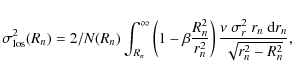
Neither the low-z nor the high-z cluster samples are spectroscopically complete to a given magnitude. Incompleteness is not a problem in the dynamical analysis as far as it is the same at all radii. In fact, the normalization of the galaxy number density profile cancels out in the Jeans procedure (see Eqs. (3) and (4) in Sect. 4) and the shape of the galaxy number-density and velocity-dispersion profiles are known to be independent from the galaxy luminosities, at least for absolute magnitudes M_R > -22.8 (Biviano et al. 2002). Galaxies brighter than M_R=-22.8 are mostly BCGs, and have been mostly excluded from our samples by removing the very central cluster regions, R_n < 0.05. While there are several indications that dwarf galaxies in clusters have a different phase-space distribution from bright galaxies (e.g., Lobo et al. 1997; Odell et al. 2002; Popesso et al. 2006; Kambas et al. 2000), this is irrelevant here since dwarf galaxies are not present in our samples.

If incompleteness does depend on radius, a correction must be applied. In fact, a radially-dependent incompleteness would change not only the normalization of the galaxy density profile but also its shape. For the ENACS, from which our local sample is extracted, it has been shown that the spectroscopic incompleteness is not radial dependent (Katgert et al. 1998). On the other hand, for the high-z cluster sample spectroscopic incompleteness is a function of radius, although not a strong one, and must be corrected for (Poggianti et al. 2006). The incompleteness correction for each cluster in our high-z sample is done by applying the geometrical weights with the method described in Poggianti et al. (2006, Appendix A).

Another kind of radial incompleteness results from the stacking procedure when the clusters that enter the stacked sample do not cover the same radial range, i.e. they have not all been sampled out to the same limiting aperture. This happens for both our local and distant samples (the apertures are listed in the last column of Tables 1 and 2). A radical way of addressing this problem would be to stack clusters only out to the minimum among all clusters apertures. In order to make the most efficient use of our sample, and explore the clusters dynamics out to r₂₀₀, we prefer to follow another approach. We apply a correction for the fact that not all clusters contribute at all radii. This correction is based on the relative individual cluster contributions to the total number of galaxies in the stacked sample, estimated at the radii where the clusters are still sampled. E.g. if at a given radius R_n,m, there are m clusters that have not been sampled out to that radius, their contributions at radii R_n>R_n,m is accounted for by applying a correction factor $1/(1-\sum_{i=1}^{m} f_i)$ to the total galaxy counts in the stacked cluster, where f_i is the fraction of galaxies contributed to the total sample by cluster i in the radial range where the cluster is sampled. The method is similar to the one described in Merrifield & Kent (1989) and has been applied to the ENACS sample in Biviano et al. (2002) and Katgert et al. (2004).

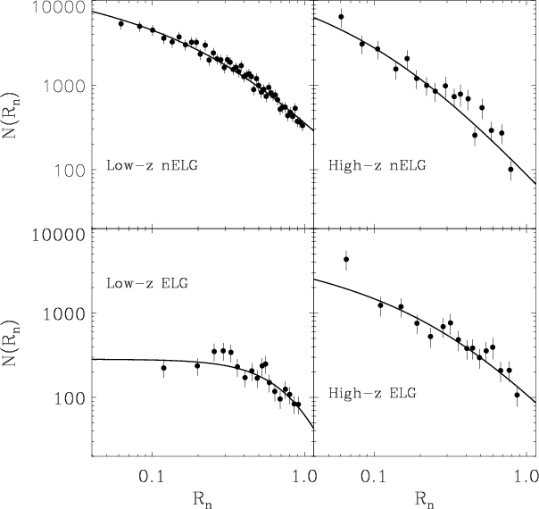$\begin{figure} \resizebox{9cm}{!}{\includegraphics{11757f1.ps}} \end{figure}$	Figure 1: The projected number density profiles, N(R_n), of the nELGs and ELGs ( upper and lower panel, respectively) for the low- and high-z stacked clusters ( left and right panel, respectively). Solid lines represent best-fit models to the data, i.e. projected NFW models for nELGs and high-z ELGs, and the core model for low-z ELGs (see Sect. 5.1 and 5.2).
Open with DEXTER

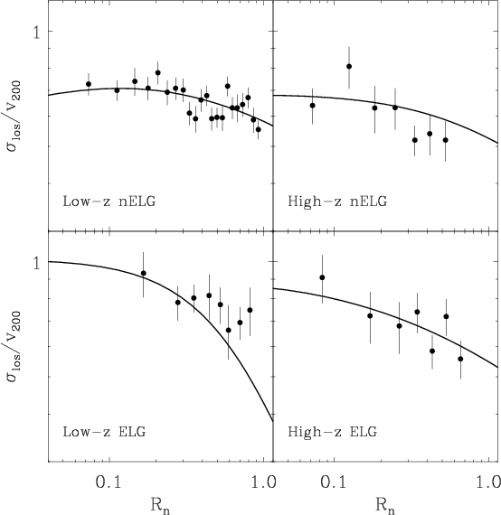$\begin{figure} \resizebox{9cm}{!}{\includegraphics{11757f2.ps}} \end{figure}$

Figure 2:

The los velocity dispersion profiles $\sigma _{\rm los}$ (R_n), of the nELGs and ELGs ( upper and lower panel, respectively) for the low- and high-z stacked cluster ( left and right panel, respectively). Solid lines represent best-fit models to the data, i.e. c=4.0 NFW mass model, a=3.6 (respectively a=1.2) OM velocity-anisotropy model for low-z nELGs (respectively, ELGs), and c=3.2 NFW mass model, a=0.01 M velocity-anisotropy model for high-z nELGs and ELGs (see Sects. 5.1 and 5.2).

Open with DEXTER

In Figs. 1 and 2 we display the projected number density profiles, N(R_n), and the los velocity dispersion profiles, $\sigma_{\rm los}(R_n)$ , respectively, of nELGs and ELGs for our local and distant stacked clusters.

4 The dynamical analysis: method

The method we adopt for the dynamical analysis of our two stacked clusters is based on the standard spherically-symmetric Jeans analysis (Binney & Tremaine 1987).

The assumption of spherical symmetry appears justified by the fact that our samples combine many clusters together, irrespective of their orientation (see also Katgert et al. 2004; van der Marel et al. 2000). The resulting stacked clusters are spherically symmetric by construction, except if the cluster selection process favors a preferential orientation. E.g., it has been argued that clusters selected because of the presence of gravitational arcs are more likely to have their major axes aligned along the los (e.g. Allen 1998). Neither ENACS nor EDisCS clusters were selected because of the presence of gravitational arcs, and they are both likely to be representative of the overall cluster populations in their mass and redshift ranges. ENACS clusters are drawn from the catalog of rich clusters in Abell et al. (1989). The mass function derived using clusters from this catalog is similar to that obtained using X-ray selected clusters (Mazure et al. 1996), hence rich clusters from the Abell et al. (1989) catalog appear to be representative of all rich clusters in the nearby universe. EDisCS clusters were optically selected from the highest surface brightness candidates in the Las Campanas Distant Cluster Survey (Gonzalez et al. 2001). From a comparison with other published optical/X-ray cluster catalogs, Gonzalez et al. (2001) have shown that their detection method is able to recover >90% of the cluster population. Further support against a possible orientation bias comes from the comparison of different EDisCS cluster mass-estimates, obtained using the distribution of cluster galaxies, gravitationally lensed images (Clowe et al. 2006; Milvang-Jensen et al. 2008) and the X-ray emission from the intra-cluster plasma (Johnson et al. 2006).

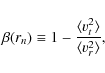
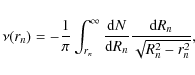
In the spherically-symmetric Jeans analysis, our observables are the galaxy number density profile N(R_n) and the los velocity dispersion profile $\sigma_{\rm los}(R_n)$ . N(R_n) is uniquely related to the 3-dimensional (3-d) galaxy number density profile $\nu(r_n)$ via the Abel inversion equation,

$\begin{displaymath}\nu(r_n) = - \frac{1}{\pi} \int_{r_n}^{\infty} \frac{{\rm d}N}{{\rm d}R_n} \frac{{\rm d}R_n}{\sqrt{R_n^2-r_n^2}}, \end{displaymath}$

(1)

where $r_n \equiv r/r_{200}$ is the 3-d clustercentric radius in normalized units. The other observable, $\sigma_{\rm los}(R_n)$ is related to the cluster mass profile, M(r_n), and the cluster velocity anisotropy profile,

$\begin{displaymath}\beta(r_n) \equiv 1 - \frac{{\langle} v_t^2 {\rangle}}{{\langle} v_r^2 {\rangle}}, \end{displaymath}$

(2)

where ${\langle} v_t^2 {\rangle}$ , ${\langle} v_r^2 {\rangle}$ are the mean squared tangential and radial velocity components, which reduce to $\sigma_t^2$ and $\sigma_r^2$ respectively, in the absence of bulk motions and net rotation. Given M(r_n) and $\beta (r_n)$ , the observable $\sigma_{\rm los}(R_n)$ follows through (van der Marel 1994)

$\begin{displaymath}\sigma_r^2(r_n) = G/\nu(r_n) \int_{r_n}^{\infty} \frac{\nu ~... ...nt_{r_n}^{\xi} \frac{\beta ~ {\rm d}x}{x}\right] {\rm d} \xi, \end{displaymath}$

(3)

and (Binney & Mamon 1982)

$\begin{displaymath}\sigma_{\rm los}^2(R_n) = 2/N(R_n) \int_{R_n}^{\infty} \left... ...frac{\nu ~ \sigma_r^2 ~ r_n ~ {\rm d}r_n}{\sqrt{r_n^2-R_n^2}}, \end{displaymath}$

(4)

where G is the gravitational constant. Note that in practice the upper limit of the integrals in the above equations is set to a finite radius (typically 20 in the integration units), large enough as to ensure that the result of the integration does not change significantly by pushing the limit to larger values.

It is therefore possible to adopt parameterized model representations of M(r_n) and $\beta (r_n)$ and determine the best-fit parameters by comparing the observed $\sigma_{\rm los}(R_n)$ profile with the predicted one, using the $\chi ^2$ statistics and the uncertainties on the observed profile.

From the eqs. above it is however clear that different combinations of the mass and anisotropy profiles can produce the same los velocity dispersion profile, the so-called ``mass-anisotropy'' degeneracy. Different methods exist to solve this degeneracy (see, e.g., Merritt 1987; Wu & Tremaine 2006; okas & Mamon 2003; van der Marel et al. 2000). These methods are effective for data-sets of ${\sim}1000$ tracers of the gravitational potential. Given the smaller size of our distant clusters data-set we here adopt another method, recently suggested by Battaglia et al. (2008) for application to the case of dwarf galaxies.

The method of Battaglia et al. (2008) consists in considering not one, but two different tracers of the cluster gravitational potential, so that there are two observables (the los velocity dispersion profiles of the two tracers) to solve for the two unknowns, M(r_n) and $\beta (r_n)$ . Since M(r_n) must be the same for both tracers, but $\beta (r_n)$ can in principle be different, the degeneracy is only partially broken, however the constraints on the dynamics of the system are significantly stronger than with a single tracer. Of course, this method works only if the two tracers have different projected phase-space distributions. This is the case of cluster nELGs and ELGs, which we therefore adopt as our two populations of tracers.

In practice, we adopt parameterized models for M(r_n) and $\beta (r_n)$ , solve Eqs. (1), (3), and (4) separately for nELGs and ELGs in each of the two stacked clusters, and jointly compare the solutions to the observed $\sigma_{\rm los}(R_n)$ of the two galaxy populations. Say $\sigma_{{\rm obs},i}$ and $\sigma_{{\rm model},i}$ the observed and predicted $\sigma _{\rm los}$ of a given population of tracers (nELG or ELG), in the ith of m radial bins, and say $\delta_i$ the corresponding 1- $\sigma$ uncertainty on $\sigma_{{\rm obs},i}$ . We find the best-fit parameter of the model representing M(r_n) and its uncertainties by minimizing

$\begin{displaymath}\chi^2 = \chi^2_{n\rm ELG} + \chi^2_{\rm ELG} \end{displaymath}$

(5)

with

$\begin{displaymath}\chi^2_{\rm tracer} = \sum_{i}^{m} (\sigma_{{\rm obs},i} - \sigma_{{\rm model},i})^2/\delta_i^2. \end{displaymath}$

(6)

Since M(r_n) must be unique for the two populations, we then adopt the joint best-fit solution for M(r_n) and solve again Eqs. (3) and (4) separately for nELGs and ELGs to determine the best-fit parameters (and uncertainties) of their $\beta$ -profiles through the $\chi ^2$ minimization, Eq. (6), i.e. we marginalize over M(r_n) to constrain the two $\beta (r_n)$ solutions.

The choice of the models cannot be too generic nor too restrictive. If it is too restrictive, we might find it difficult to find accurate fits to the data. On the other hand, with small data-sets (such as that of our high-z sample) it would be difficult to obtain strong constraints on models that are too generic or are characterized by too many parameters. We let ourselves be guided in our choices by theoretical expectations.

The distribution of mass within cosmological halos, such as galaxy clusters, is a robust prediction of the Cold Dark Matter (CDM) cosmological model. Numerical simulations have shown that all cosmological halos are characterized by the same, universal, mass density profile (Navarro et al. 1997), the so-called ``NFW'' profile,

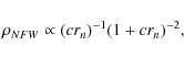$\begin{displaymath}\rho_{NFW} \propto (c r_n)^{-1} (1 + c r_n)^{-2}, \end{displaymath}$

(7)

characterized by the concentration parameter c, a central cusp, and an asymptotic slope of -3 at large radii. While other analytical forms have subsequently been proposed (see, e.g. Diemand et al. 2005; Hayashi et al. 2004; Moore et al. 1999), the NFW profile provides an acceptable fit to observed mass profiles of galaxy clusters both at low and intermediate redshifts (see, e.g. Biviano & Girardi 2003; Zappacosta et al. 2006; van der Marel et al. 2000; Katgert et al. 2004). It is therefore rather straightforward to choose the NFW profile as our reference model for M(r).

We adopt the NFW profile also as a model for $\nu(r_n)$ (actually, we fit N(R_n) with the projected NFW profile, see okas & Mamon 2001; Bartelmann 1996), but we do not make the assumption that $\nu(r_n)$ and M(r_n) are characterized by the same NFW profile. I.e. we do not work in the so-called light-traces-mass hypothesis. Whenever the NFW model does not provide an acceptable fit to $\nu(r_n)$ , we consider a different model, with one additional parameter, to allow for a better fit. The model we adopt in this case is the so-called $\beta$ -model (Cavaliere & Fusco-Femiano 1978),

$\begin{displaymath}N \propto [1+(R_n/R_c)^2]^{-\alpha}, \end{displaymath}$

(8)

characterized by two parameters, the core-radius, R_c, and the slope, $\alpha$ . In order to avoid terminology confusion with the velocity-anisotropy profile $\beta (r_n)$ , in the following we refer to the $\beta$ -model as the ``core'' model.

The model choice for the velocity-anisotropy profile $\beta (r_n)$ is less straightforward. At variance with the case of the halo mass profile, there is no claimed ``universal'' velocity anisotropy profile. We consider the two following models. One is the Mamon- $\L$ okas (``M $\L$ '' hereafter) model (Mamon & okas 2005)

$\begin{displaymath}\beta = 0.5 ~ r_n/(r_n+a), \end{displaymath}$

(9)

which has been shown to provide a good fit to the velocity anisotropy profiles of simulated cosmological halos. The other is the Osipkov-Merritt (``OM'' hereafter) model (Merritt 1985; Osipkov 1979)

$\begin{displaymath}\beta = r_n^2/(r_n^2+a^2), \end{displaymath}$

(10)

which provides a good fit to the observed velocity anisotropy profile of late-type galaxies in the ENACS sample (Biviano & Katgert 2004). Both the M $\L$ and the OM models depend on just one free parameter, the anisotropy radius, a.

5 Results

5.1 The nearby cluster sample

The NFW profile (in projection) provides an acceptable fit to the nELG N(R_n), with c=2.4. This best-fit profile is shown in the upper-left panel of Fig. 1. On the other hand, the ELG N(R) cannot be fitted by a (projected) NFW profile, because the ELGs avoid the central cluster region. The wider spatial distribution of the ELGs as compared to that of the nELGs clearly reflects the well known MDR (see Sect. 1). In order to fit the rather flat ELG N(R_n), we adopt the core model, and we find an acceptable fit with R_c=1.28 and $\alpha=-3.2$ (see the bottom-left panel of Fig. 1). The N(R_n) best-fitting models are Abel-inverted to provide the 3-d number density profiles $\nu(r_n)$ that we use in the Jeans analysis.

The observed $\sigma _{\rm los}$ -profiles of the nELGs and ELGs are shown in the upper-left and, respectively, lower-left panels of Fig. 2. The strikingly different behavior of the two $\sigma _{\rm los}$ -profiles reflects the well known morphological segregation in velocity space (see Sect. 1). We then determine the best-fit concentration parameter of a NFW M(r_n) model by a joint $\chi ^2$ comparison of the observed nELG and ELG $\sigma _{\rm los}$ -profiles with those predicted by the Jeans analysis for the given mass model, and for either M $\L$ or OM $\beta (r_n)$ models. The best-fit solution is obtained using the OM model for the velocity anisotropy profiles of nELGs and ELGs. The best-fit value of the NFW concentration parameter is c=4.0_{(-0.1) -1.3}^{(+0.5) +2.3}(90% confidence levels, c.l. in the following, 68% c.l. in brackets). The $\chi ^2$ vs. c solution is displayed in the top panel of Fig. 3.

Marginalizing over this M(r_n) best-fit solution we obtain the best-fit $\beta (r_n)$ OM-model parameters a=3.6_-1.6^+13.4 and a=1.2_-0.4^+1.2 (in units of r₂₀₀) for the nELG and ELG populations, respectively. We only provide here 90% c.l., since we find no acceptable solutions at the 68% c.l. for the ELGs. The best-fit model $\sigma _{\rm los}$ -profiles are shown as solid lines overlaid on the observed, binned $\sigma _{\rm los}$ (R_n) in Fig. 2 (left-hand panels). Clearly, the fit to the ELG $\sigma _{\rm los}$ (R_n) is not excellent, but still acceptable to within 90% c.l.

The solutions for the velocity-anisotropy profiles are displayed in Fig. 4 for the nELGs (upper-left panel) and the ELGs (lower-left panel). Notice that the quantity displayed in Fig. 4 is $\sigma _r/\sigma _t \equiv (1-\beta )^{-1/2}$ . The nELG velocity-anisotropy profile is consistent with fully isotropic orbits of this population of galaxies within the virial region, in agreement with the results obtained by Katgert et al. (2004). On the other hand, the ELG orbits are approximately isotropic only out to $r_n \simeq 0.6$ , and then become increasingly radial. The OM-model solution is very similar to the non-parametric velocity-anisotropy profile derived by Biviano & Katgert (2004). It is also quite similar to the velocity-anisotropy profiles of DM particles in cluster-size simulated halos at $z \approx 0$ (e.g. Diaferio et al. 2001; Tormen et al. 1997).

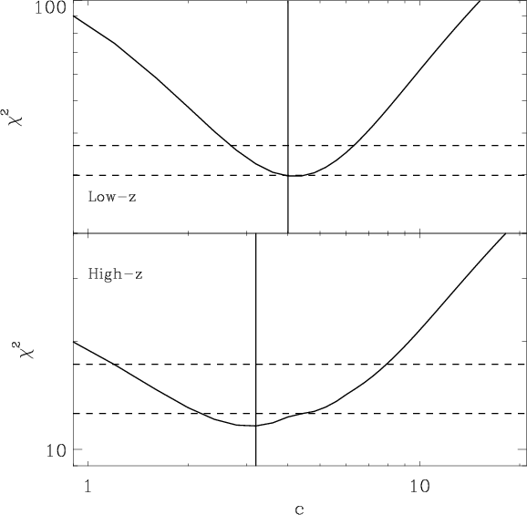$\begin{figure} \par\resizebox{9cm}{!}{\includegraphics{11757f3.ps}} \end{figure}$	Figure 3: The $\chi ^2$ values vs. the c parameter of the NFW mass profile model for our low-z ( top panel) and high-z ( bottom panel) stacked clusters. The two dashed lines indicate the 68% and 90% c.l., and the vertical lines indicate the best-fit c values.
Open with DEXTER

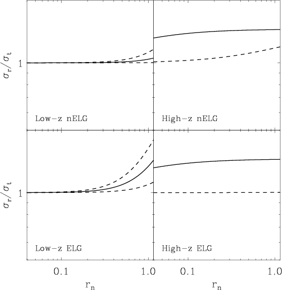$\begin{figure} \resizebox{9cm}{!}{\includegraphics{11757f4.ps}} \end{figure}$

Figure 4:

Best-fit velocity-anisotropy profile $\sigma _r/\sigma _t \equiv (1-\beta )^{-1/2}$ for nELGs ( upper left panel) and ELGs ( lower left panel) in low-z clusters and for nELGs ( upper right panel) and ELGs ( lower right panel) in high-z clusters. The best-fit velocity-anisotropy model is OM for the low-z sample and M for the high-z sample. Dashed lines indicate the 90% c.l. For the high-z sample, the best-fit solutions are at the lower-limit of the interval considered in the $\chi ^2$ minimization analysis, hence only the lower c.l. to $\beta (r_n)$ are shown.

Open with DEXTER

For the sake of comparison with the distant cluster sample (see Sect. 5.2) it is useful to also consider the solution obtained for the M $\L$ $\beta (r_n)$ model. With such a model, we obtain an acceptable solution of the Jeans analysis for a NFW mass profile with the same concentration value obtained using the OM $\beta (r_n)$ model (c=4), although with a larger $\chi ^2$ value. Marginalizing over the c=4 parameter, we then obtain the best-fit $\beta (r_n)$ M $\L$ model parameters a=2.9_-2.4^>+20 and a=1.5_-0.8^+3.4 (90% c.l.) for the nELG and ELG populations, respectively. Similarly to what is obtained using the OM $\beta (r_n)$ model, also in this case the best-fit anisotropy radius of the nELG population is about twice as large as that of the ELG population, indicating that the ELG orbits in clusters are more radially elongated than the nELG orbits.

5.2 The distant cluster sample

Both the nELG and the ELG N(R_n) are well fitted by projected NFW profiles with c=7.5 and c=2.7, respectively. These N(R_n)best-fitting models are Abel-inverted to provide the 3-d number density profiles $\nu(r_n)$ that we use in the Jeans analysis. The binned profiles and their best-fit models are shown in the right-hand panels of Fig. 1. Similarly to what is found in the nearby cluster sample, ELGs have a wider spatial distribution than nELGs, confirming previous results about the existence of a MDR also at $z \sim 0.6$ (see Sect. 1). However, the ELGs do not avoid the central cluster regions as in low-z clusters.

The evidence for segregation in velocity space is not so strong. In fact the $\sigma _{\rm los}$ -profiles of nELGs and ELGs are not very different (see the right-hand panels of Fig. 2), in contrast with the situation seen in low-z clusters. We jointly compare these $\sigma _{\rm los}$ -profiles with those predicted by NFW M(r_n)-models, and either M $\L$ or OM $\beta (r_n)$ models, via the $\chi ^2$ method described in Sect. 4. The best-fit solution is obtained for the M $\L$ $\beta (r_n)$ model. The best-fit value of the NFW concentration parameter is c=3.2_{(-1.0) -2.0}^{(+1.2) +4.6} (90% c.l., 68% c.l. in brackets). The $\chi ^2$ vs. c solution is displayed in Fig. 3, bottom panel. As expected from the smaller size of the high-z sample, the solution is less well constrained than for the low-z sample.

We then adopt the c=3.2 NFW best-fit solution as the reference M(r_n) for the stacked high-z cluster, and look for the best-fit $\beta (r_n)$ M $\L$ -model solutions, separately for nELGs and ELGs. We find that the best-fit anisotropy-radius parameter is identical for the two galaxy classes, a=0.01, at the lower limit of the a-range considered in the $\chi ^2$ minimization analysis. Unfortunately, the solutions are poorly constrained. The 90% upper limit for the nELGs is a<0.9, that for the ELGs is at the upper limit of the a-range considered, $a \leq 10.0$ . The best-fit model $\sigma _{\rm los}$ -profiles are shown as solid lines overlaid on the observed, binned $\sigma _{\rm los}$ (r_n) in Fig. 2 (right-hand panels).

The solutions for the velocity-anisotropy profiles, $\sigma_r/\sigma_t$ , are displayed in Fig. 4 (right-hand panels) and are identical for the nELGs and the ELGs. The upper limits on the a-parameters translate in lower-envelopes to the velocity-anisotropy profiles (dashed curves in the right-hand panels of Fig. 4). Taken at face value, both the nELGs and the ELGs have radially anisotropic orbits. Isotropic orbits are excluded for high-z nELGs, at least outside the center, but cannot be excluded for high-z ELGs because of the large error bars.

The poor constraints on the velocity anisotropy of high-z ELGs do not allow us to draw any conclusion about their orbital evolution with z. Taken at face value the results suggest that ELGs follow radially anisotropic orbits both in high-z and in low-z clusters. On the other hand, the orbits of nELGs evolve with z, from almost isotropic in low-z clusters to radially anisotropic in high-z clusters (compare the left-hand and right-hand panels of Fig. 4).

6 Summary and discussion

We have obtained acceptable equilibrium solutions to the nELG and ELG projected phase-space distributions with NFW M(r_n) models, and with OM and, respectively, M $\L$ $\beta (r_n)$ models, for the low-z and, respectively, the high-z sample. The solutions do not always provide excellent fits to the $\sigma _{\rm los}$ (R_n) of the nELGs and ELGs, but they are anyway always acceptable at the 90% c.l. Hence, the rather limited set of models we have considered seems to be adequate for our data-sets. Larger data-sets would be required if a wider range of models and/or parameters is to be considered.

The best-fit NFW c values found with the Jeans analysis are in agreement with those expected in a $\Lambda$ CDM universe for cosmological halos with the masses and redshifts of the clusters in our samples. In Fig. 5 we display the distribution of the predicted c values for the clusters in the low-z and high-zsamples. The predicted c values are obtained from our cluster mass and redshift estimates, using the c=c(M,z) relations of Gao et al. (2008) and Duffy et al. (2008). In the same figure we also display the best-fit c value obtained with the Jeans analysis, and the 68 and 90% c.l. The Jeans solutions are fully consistent with the predicted distributions of c values, both at low- and at high-z.

Duffy et al. (2008) claimed that a discrepancy exists between the predicted c values for groups and clusters of galaxies and those determined observationally using X-ray observations. Since this is not apparent here, the claimed discrepancy may occur mostly at the group scale (see Fig. 8 in Biviano 2008) or originate from a systematic bias in the the X-ray-based cluster mass estimates (Rasia et al. 2006).

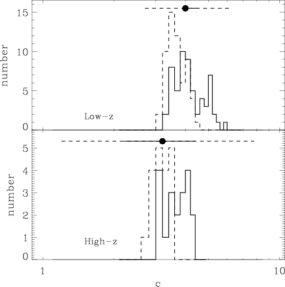$\begin{figure} \resizebox{9cm}{!}{\includegraphics{11757f5.ps}} \end{figure}$

Figure 5:

The distributions of predicted c for the low-z ( upper panel) and high-z ( lower panel) cluster samples, as obtained from the relation of Gao et al. (2008) (solid histograms) and Duffy et al. (2008) (dashed histograms) applied to our cluster mass and redshift estimates. The dots indicate the best-fit c values from the Jeans analysis, and the solid and dashed lines above the histograms the 68%, respectively 90%, confidence intervals on the best-fit solutions.

Open with DEXTER

Our results are therefore consistent with the theoretical c=c(M,z) relation for cosmological cluster-sized halos in a $\Lambda$ CDM universe.

As far as the orbits of cluster galaxies are concerned, our analysis suggests that these orbits become more isotropic with time. Low-zcluster nELGs have nearly isotropic orbits, low-z cluster ELGs have radially anisotropic orbits outside the central cluster regions. We can exclude that ELGs follow isotropic orbits at the 90% c.l. outside $r \simeq 0.6 ~ r_{200}$ .

In high-z clusters nELGs and ELGs appear to be characterized by similar orbital anisotropies, radial and almost constant with radius. For nELGs we can exclude isotropic orbits outside $r \simeq 0.1 ~ r_{200}$ at the 90% c.l. Since low-z cluster nELGs are characterized by nearly isotropic orbits, the orbits of nELGs must evolve from radial to isotropic with time. No significant evolution is found for the orbits of ELGs, which remain radially anisotropic both at high- and low-z.

A process capable of isotropizing galaxy orbits with time is the secular growth of cluster mass via hierarchical accretion (Gill et al. 2004). According to theoretical models, the growth of halo masses occurs in two phases, an initial, fast accretion phase, followed by a slower, smoother accretion phase (Lapi & Cavaliere 2009). During the fast accretion phase clusters undergo major mergers that can induce rapid changes in the cluster gravitational potential (Valluri et al. 2007; Manrique et al. 2003; Peirani et al. 2006), causing energy and angular momentum mixing in the galaxy distributions, and thereby isotropization of galaxy orbits (Lynden-Bell 1967; Merritt 2005; Lapi & Cavaliere 2009; Kandrup & Siopis 2003; Hénon 1964).

Cluster-sized halos of $10^{14{-}15} ~ M_{\odot}$ mass undergo the transition from the fast to the slow accretion phase at $z \approx 0.4$ (see Fig.6 in Lapi & Cavaliere 2009). Hence, clusters in our high-zsample are observed before the end of their fast accretion phase. During this phase, the orbits of cluster galaxies can still evolve, approaching isotropy. At z<0.4 one therefore expects to see isotropic orbits for those galaxies that were already part of the clusters before the end of the fast accretion phase. In our low-zcluster sample we therefore expect nELGs to be characterized by isotropic orbits, as observed. On the other hand, ELGs must be newcomers in low-z clusters, hence memory of their recent cluster infall is still conserved in their (radially elongated) orbits.

The fact that a significant fraction ( $23 \pm 3$ %, Poggianti et al. 2009) of the high-z nELGs have a k+a or a+kspectral classification is supporting evidence for the fact that the clusters of our high-z sample are still in the fast accretion phase. The spectral characteristics of these galaxies are in fact indicative that their star formation have stopped in the ${\sim} 1.5$ Gyr prior to observation (Poggianti et al. 1999). If the cessation of the star-formation activity in these galaxies is related to their first encounter with the cluster environment, their accretion has been relatively recent. Hence, a large part of the cluster galaxies (and presumably, of the cluster mass) has been assembled in the last ${\sim} 1.5$ Gyr.

The detected orbital evolution occurs over the same period of cosmic time (the last ${\sim} 5$ Gyr) when the cluster galaxy population undergoes a major change in its morphological mix (Desai et al. 2007) and star formation properties (Poggianti et al. 2006). We might then be witnessing two effects of the same underlying physical phenomenon.

The transformation of ELGs into nELGs may be at least partly responsible for another evolutionary trend we observe in our clusters, that of the nELG number density profile. This profile becomes less concentrated with time, an evolution in the opposite sense to that observed for the mass density profile. The (projected) NFW models fitted to the number density profile of low- and high-z nELGs have best-fit concentrations c=2.4_-0.2^+0.6 and c=7.5_-0.9^+1.6 (90% c.l., see also Fig. 1). On the other hand, no significant evolution is found for the number density profile of nELGs and ELGs together. This profile is dominated by nELGs at low-z, but not at high-z. If high-z ELGs transform into nELGs with time, the nELG+ELG number density profile would not change, but the nELG number density profile would flatten, since ELGs are less spatially concentrated than nELGs. Also the ELG number density profile flattens with time. This might be related to the cluster environment growing more hostile with time, and making more difficult for infalling field galaxies to conserve their gas as they approach and cross the cluster centers.

The results we have obtained in the present study are based on the still rather limited amount of available data for high-z cluster galaxies. Moreover, our high-z and low-z cluster samples span quite a substantial range in masses. It will then be important to tighten the current constraints on the orbital evolution of cluster galaxies using future, larger spectroscopic data-sets for high-zclusters, and also to re-assess such an evolution as a function of cluster mass. From these future analyses we will obtain a more thorough understanding of the hierarchical assembly history and evolution of galaxy clusters.

Acknowledgements

We acknowledge useful discussions with Giuseppina Battaglia, Alfonso Cavaliere and Gary Mamon. We thank the anonymous referee for her/his useful remarks. This research has been financially supported from the National Institute for Astrophysics through the PRIN-INAF scheme. This research has made use of NASA's Astrophysics Data System.

References

Abell, G. O., Corwin, Jr., H. G., & Olowin, R. P. 1989, ApJS, 70, 1 [NASA ADS] [CrossRef] (In the text)
Adami, C., Biviano, A., & Mazure, A. 1998a, A&A, 331, 439 [NASA ADS]
Adami, C., Mazure, A., Katgert, P., & Biviano, A. 1998b, A&A, 336, 63 [NASA ADS] (In the text)
Adami, C., Biviano, A., Durret, F., & Mazure, A. 2005, A&A, 443, 17 [NASA ADS] [CrossRef] [EDP Sciences] (In the text)
Allen, S. W. 1998, MNRAS, 296, 392 [NASA ADS] [CrossRef] (In the text)
Bartelmann, M. 1996, A&A, 313, 697 [NASA ADS]
Battaglia, G., Helmi, A., Tolstoy, E., et al. 2008, ApJ, 681, L13 [NASA ADS] [CrossRef] (In the text)
Beers, T. C., Flynn, K., & Gebhardt, K. 1990, AJ, 100, 32 [NASA ADS] [CrossRef] (In the text)
Benatov, L., Rines, K., Natarajan, P., Kravtsov, A., & Nagai, D. 2006, MNRAS, 370, 427 [NASA ADS] (In the text)
Binney, J., & Mamon, G. A. 1982, MNRAS, 200, 361 [NASA ADS] (In the text)
Binney, J., & Tremaine, S. 1987, Galactic dynamics (Princeton, NJ: Princeton University Press)
Biviano, A. 2000, in Constructing the Universe with Clusters of Galaxies, http://nedwww.ipac.caltech.edu/level5/Biviano2/frames.html (In the text)
Biviano, A. 2006 [arXiv:astro-ph/0607040] (In the text)
Biviano, A. 2008 [arXiv:0811.3535]
Biviano, A., & Girardi, M. 2003, ApJ, 585, 205 [NASA ADS] [CrossRef]
Biviano, A., & Katgert, P. 2004, A&A, 424, 779 [NASA ADS] [CrossRef] [EDP Sciences] (In the text)
Biviano, A., Girardi, M., Giuricin, G., Mardirossian, F., & Mezzetti, M. 1992, ApJ, 396, 35 [NASA ADS] [CrossRef]
Biviano, A., Katgert, P., Mazure, A., et al. 1997, A&A, 321, 84 [NASA ADS]
Biviano, A., Katgert, P., Thomas, T., & Adami, C. 2002, A&A, 387, 8 [NASA ADS] [CrossRef] [EDP Sciences] (In the text)
Biviano, A., Murante, G., Borgani, S., et al. 2006, A&A, 456, 23 [NASA ADS] [CrossRef] [EDP Sciences] (In the text)
Carlberg, R. G., Yee, H. K. C., Ellingson, E., et al. 1997a, ApJ, 485, L13 [NASA ADS] [CrossRef]
Carlberg, R. G., Yee, H. K. C., Ellingson, E., et al. 1997b, ApJ, 476, L7 [NASA ADS] [CrossRef]
Cavaliere, A., & Fusco-Femiano, R. 1978, A&A, 70, 677 [NASA ADS] (In the text)
Clowe, D., Shneider, P., Aragón-Salamanca, A., et al. 2006, A&A, 451, 395 [NASA ADS] [CrossRef] [EDP Sciences]
De Lucia, G., & Blaizot, J. 2007, MNRAS, 375, 2 [NASA ADS] [CrossRef]
den Hartog, R., & Katgert, P. 1996, MNRAS, 279, 349 [NASA ADS] (In the text)
Desai, V., Dalcanton, J. J., Aragón-Salamanca, A., et al. 2007, ApJ, 660, 1151 [NASA ADS] [CrossRef] (In the text)
Diaferio, A., Kauffmann, G., Balogh, M. L., et al. 2001, MNRAS, 323, 999 [NASA ADS] [CrossRef]
Diemand, J., Zemp, M., Moore, B., Stadel, J., & Carollo, C. M. 2005, MNRAS, 364, 665 [NASA ADS]
Dolag, K., Bartelmann, M., Perrotta, F., et al. 2004, A&A, 416, 853 [NASA ADS] [CrossRef] [EDP Sciences]
Dressler, A. 1980, ApJ, 236, 351 [NASA ADS] [CrossRef] (In the text)
Dressler, A., Oemler, A. J., Couch, W. J., et al. 1997, ApJ, 490, 577 [NASA ADS] [CrossRef]
Dressler, A., Smail, I., Poggianti, B. M., et al. 1999, ApJS, 122, 51 [NASA ADS] [CrossRef]
Duffy, A. R., Schaye, J., Kay, S. T., & Dalla Vecchia, C. 2008, MNRAS, 390, L64 [NASA ADS] (In the text)
Fasano, G., Poggianti, B. M., Couch, W. J., et al. 2000, ApJ, 542, 673 [NASA ADS] [CrossRef]
Gao, L., Navarro, J. F., Cole, S., et al. 2008, MNRAS, 387, 536 [NASA ADS] [CrossRef] (In the text)
Gill, S. P. D., Knebe, A., Gibson, B. K., & Dopita, M. A. 2004, MNRAS, 351, 410 [NASA ADS] [CrossRef] (In the text)
Girardi, M., Biviano, A., Giuricin, G., Mardirossian, F., & Mezzetti, M. 1993, ApJ, 404, 38 [NASA ADS] [CrossRef] (In the text)
Gonzalez, A. H., Zaritsky, D., Dalcanton, J. J., & Nelson, A. 2001, ApJS, 137, 117 [NASA ADS] [CrossRef] (In the text)
Halliday, C., Milvang-Jensen, B., Porier, S., et al. 2004, A&A, 427, 397 [NASA ADS] [CrossRef] [EDP Sciences]
Harrison, E. R., & Noonan, T. W. 1979, ApJ, 232, 18 [NASA ADS] [CrossRef] (In the text)
Hayashi, E., Navarro, J. F., Power, C., et al. 2004, MNRAS, 355, 794 [NASA ADS] [CrossRef]
Hénon, M. 1964, Annales d'Astrophysique, 27, 83 [NASA ADS]
Johnson, O., Best, P., Zaritsky, D., et al. 2006, MNRAS, 371, 1777 [NASA ADS] [CrossRef] (In the text)
Kambas, A., Davies, J. I., Smith, R. M., Bianchi, S., & Haynes, J. A. 2000, AJ, 120, 1316 [NASA ADS] [CrossRef]
Kandrup, H. E., & Siopis, C. 2003, MNRAS, 345, 727 [NASA ADS] [CrossRef]
Katgert, P., Mazure, A., Perea, J., et al. 1996, A&A, 310, 8 [NASA ADS]
Katgert, P., Mazure, A., den Hartog, R., et al. 1998, A&AS, 129, 399 [NASA ADS] [CrossRef] [EDP Sciences]
Katgert, P., Biviano, A., & Mazure, A. 2004, ApJ, 600, 657 [NASA ADS] [CrossRef] (In the text)
Lapi, A., & Cavaliere, A. 2009, ApJ, 692, 174 [NASA ADS] [CrossRef] (In the text)
Lobo, C., Biviano, A., Durret, F., et al. 1997, A&A, 317, 385 [NASA ADS]
okas, E. L., & Mamon, G. A. 2001, MNRAS, 321, 155 [NASA ADS] [CrossRef]
okas, E. L., & Mamon, G. A. 2003, MNRAS, 343, 401 [NASA ADS] [CrossRef]
Lynden-Bell, D. 1967, MNRAS, 136, 101 [NASA ADS]
Mamon, G. A., & okas, E. L. 2005, MNRAS, 363, 705 [NASA ADS] [CrossRef] (In the text)
Manrique, A., Raig, A., Salvador-Solé, E., Sanchis, T., & Solanes, J. M. 2003, ApJ, 593, 26 [NASA ADS] [CrossRef]
Mauduit, J.-C., & Mamon, G. A. 2007, A&A, 475, 169 [NASA ADS] [CrossRef] [EDP Sciences] (In the text)
Mazure, A., Katgert, P., den Hartog, R., et al. 1996, A&A, 310, 31 [NASA ADS] (In the text)
Menci, N., & Fusco-Femiano, R. 1996, ApJ, 472, 46 [NASA ADS] [CrossRef] (In the text)
Merrifield, M. R., & Kent, S. M. 1989, AJ, 98, 351 [NASA ADS] [CrossRef] (In the text)
Merritt, D. 1985, MNRAS, 214, 25P [NASA ADS]
Merritt, D. 1987, ApJ, 313, 121 [NASA ADS] [CrossRef]
Merritt, D. 2005, New York Academy Sciences Annals, 1045, 3 [NASA ADS] [CrossRef]
Milvang-Jensen, B., Noll, S., Halliday, C., et al. 2008, A&A, 482, 419 [NASA ADS] [CrossRef] [EDP Sciences] (In the text)
Moore, B., Quinn, T., Governato, F., Stadel, J., & Lake, G. 1999, MNRAS, 310, 1147 [NASA ADS] [CrossRef]
Moss, C., & Dickens, R. J. 1977, MNRAS, 178, 701 [NASA ADS]
Navarro, J. F., Frenk, C. S., & White, S. D. M. 1997, ApJ, 490, 493 [NASA ADS] [CrossRef] (In the text)
Odell, A. P., Schombert, J., & Rakos, K. 2002, AJ, 124, 3061 [NASA ADS] [CrossRef]
Osipkov, L. P. 1979, Sov. Astron. Lett., 5, 42 [NASA ADS]
Peirani, S., Durier, F., & de Freitas Pacheco, J. A. 2006, MNRAS, 367, 1011 [NASA ADS] [CrossRef]
Poggianti, B. M., Aragón-Salamanca, A., Zaritsky, D., et al. 2009, ApJ, 693, 112 [NASA ADS] [CrossRef] (In the text)
Poggianti, B. M., Smail, I., Dressler, A., et al. 1999, ApJ, 518, 576 [NASA ADS] [CrossRef]
Poggianti, B. M., von der Linden, A., De Lucia, G., et al. 2006, ApJ, 642, 188 [NASA ADS] [CrossRef]
Popesso, P., Biviano, A., Böhringer, H., & Romaniello, M. 2006, A&A, 445, 29 [NASA ADS] [CrossRef] [EDP Sciences]
Postman, M., Franx, M., Cross, N. J. G., et al. 2005, ApJ, 623, 721 [NASA ADS] [CrossRef]
Ramella, M., Biviano, A., Pisani, A., et al. 2007, A&A, 470, 39 [NASA ADS] [CrossRef] [EDP Sciences]
Rasia, E., Ettori, S., Moscardini, L., et al. 2006, MNRAS, 369, 2013 [NASA ADS] [CrossRef] (In the text)
Rines, K., Geller, M. J., Kurtz, M. J., & Diaferio, A. 2003, AJ, 126, 2152 [NASA ADS] [CrossRef]
Rines, K., Finn, R., & Vikhlinin, A. 2007, ApJ, 665, L9 [NASA ADS] [CrossRef]
Smith, G. P., Treu, T., Ellis, R. S., Moran, S. M., & Dressler, A. 2005, ApJ, 620, 78 [NASA ADS] [CrossRef]
Sodré, L. J., Capelato, H. V., Steiner, J. E., & Mazure, A. 1989, AJ, 97, 1279 [NASA ADS] [CrossRef]
Tammann, G. A. 1972, A&A, 21, 355 [NASA ADS]
Tormen, G., Bouchet, F. R., & White, S. D. M. 1997, MNRAS, 286, 865 [NASA ADS]
Valluri, M., Vass, I. M., Kazantzidis, S., Kravtsov, A. V., & Bohn, C. L. 2007, ApJ, 658, 731 [NASA ADS] [CrossRef]
van der Marel, R. P. 1994, MNRAS, 270, 271 [NASA ADS] (In the text)
van der Marel, R. P., Magorrian, J., Carlberg, R. G., Yee, H. K. C., & Ellingson, E. 2000, AJ, 119, 2038 [NASA ADS] [CrossRef] (In the text)
White, S. D. M., Clowe, D. I., Simard, L., et al. 2005, A&A, 444, 365 [NASA ADS] [CrossRef] [EDP Sciences] (In the text)
Whitmore, B. C., Gilmore, D. M., & Jones, C. 1993, ApJ, 407, 489 [NASA ADS] [CrossRef] (In the text)
Wojtak, R., okas, E. L., Mamon, G. A., et al. 2007, A&A, 466, 437 [NASA ADS] [CrossRef] [EDP Sciences]
Wu, X., & Tremaine, S. 2006, ApJ, 643, 210 [NASA ADS] [CrossRef]
Zappacosta, L., Buote, D. A., Gastaldello, F., et al. 2006, ApJ, 650, 777 [NASA ADS] [CrossRef]

Footnotes

...)

The virial radius r₂₀₀ is the radius within which the enclosed average mass density of a cluster is 200 times the critical density.

The virial mass M₂₀₀ is the mass enclosed within a sphere of radius r₂₀₀.

The circular velocity is defined from the previous two quantities as v₂₀₀ = (G M₂₀₀/r₂₀₀)^1/2.

All Tables

Table 1: The low-z cluster sample.

Table 2: The high-z cluster sample.

All Figures

$\begin{figure} \resizebox{9cm}{!}{\includegraphics{11757f1.ps}} \end{figure}$	Figure 1: The projected number density profiles, N(R_n), of the nELGs and ELGs ( upper and lower panel, respectively) for the low- and high-z stacked clusters ( left and right panel, respectively). Solid lines represent best-fit models to the data, i.e. projected NFW models for nELGs and high-z ELGs, and the core model for low-z ELGs (see Sect. 5.1 and 5.2).
Open with DEXTER
In the text

$\begin{figure} \resizebox{9cm}{!}{\includegraphics{11757f2.ps}} \end{figure}$	Figure 2: The los velocity dispersion profiles $\sigma _{\rm los}$ (R_n), of the nELGs and ELGs ( upper and lower panel, respectively) for the low- and high-z stacked cluster ( left and right panel, respectively). Solid lines represent best-fit models to the data, i.e. c=4.0 NFW mass model, a=3.6 (respectively a=1.2) OM velocity-anisotropy model for low-z nELGs (respectively, ELGs), and c=3.2 NFW mass model, a=0.01 M velocity-anisotropy model for high-z nELGs and ELGs (see Sects. 5.1 and 5.2).
Open with DEXTER
In the text

$\begin{figure} \par\resizebox{9cm}{!}{\includegraphics{11757f3.ps}} \end{figure}$	Figure 3: The $\chi ^2$ values vs. the c parameter of the NFW mass profile model for our low-z ( top panel) and high-z ( bottom panel) stacked clusters. The two dashed lines indicate the 68% and 90% c.l., and the vertical lines indicate the best-fit c values.
Open with DEXTER
In the text

$\begin{figure} \resizebox{9cm}{!}{\includegraphics{11757f4.ps}} \end{figure}$	Figure 4: Best-fit velocity-anisotropy profile $\sigma _r/\sigma _t \equiv (1-\beta )^{-1/2}$ for nELGs ( upper left panel) and ELGs ( lower left panel) in low-z clusters and for nELGs ( upper right panel) and ELGs ( lower right panel) in high-z clusters. The best-fit velocity-anisotropy model is OM for the low-z sample and M for the high-z sample. Dashed lines indicate the 90% c.l. For the high-z sample, the best-fit solutions are at the lower-limit of the interval considered in the $\chi ^2$ minimization analysis, hence only the lower c.l. to $\beta (r_n)$ are shown.
Open with DEXTER
In the text

$\begin{figure} \resizebox{9cm}{!}{\includegraphics{11757f5.ps}} \end{figure}$	Figure 5: The distributions of predicted c for the low-z ( upper panel) and high-z ( lower panel) cluster samples, as obtained from the relation of Gao et al. (2008) (solid histograms) and Duffy et al. (2008) (dashed histograms) applied to our cluster mass and redshift estimates. The dots indicate the best-fit c values from the Jeans analysis, and the solid and dashed lines above the histograms the 68%, respectively 90%, confidence intervals on the best-fit solutions.
Open with DEXTER
In the text

Current usage metrics show cumulative count of Article Views (full-text article views including HTML views, PDF and ePub downloads, according to the available data) and Abstracts Views on Vision4Press platform.

Data correspond to usage on the plateform after 2015. The current usage metrics is available 48-96 hours after online publication and is updated daily on week days.

Initial download of the metrics may take a while.