Pre-recombinational energy release and narrow features in the CMB spectrum

J. Chluba; R. A. Sunyaev

doi:10.1051/0004-6361/200809840

Free Access

Issue		A&A Volume 501, Number 1, July I 2009


Page(s)		29 - 47
Section		Cosmology (including clusters of galaxies)
DOI		https://doi.org/10.1051/0004-6361/200809840
Published online		05 May 2009

Pre-recombinational energy release and narrow features in the CMB spectrum

J. Chluba¹ - R. A. Sunyaev^1,2

1 - Max-Planck-Institut für Astrophysik, Karl-Schwarzschild-Str. 1, 85741 Garching bei München, Germany
2 - Space Research Institute, Russian Academy of Sciences, Profsoyuznaya 84/32, 117997 Moscow, Russia

Received 25 March 2008 / Accepted 27 February 2009

Abstract
Energy release in the early Universe ( $z\la 2 \times 10^{6}$ ) should produce a broad spectral distortion of the cosmic microwave background (CMB) radiation field, which can be characterized as y-type distortion when the injection process started at redshifts $z\la 5 \times 10^{4}$ . Here we demonstrate that if energy was released before the beginning of cosmological hydrogen recombination ( $z\sim 1400$ ), closed loops of bound-bound and free-bound transitions in H I and He II lead to the appearance of (i) characteristic multiple narrow spectral features at dm and cm wavelengths; and (ii) a prominent sub-millimeter feature consisting of absorption and emission parts in the far Wien tail of CMB spectrum. The additional spectral features are generated in the pre-recombinational epoch of H I ( $z\ga 1800$ ) and He II ( $z\ga 7000$ ), and therefore differ from those arising due to normal cosmological recombination in the undisturbed CMB blackbody radiation field. We present the results of numerical computations including 25 atomic shells for both H I and He II, and discuss the contributions of several individual transitions in detail. As examples, we consider the case of instantaneous energy release (e.g., due to phase transitions), and exponential energy release (e.g., because of long-lived decaying particles). Our computations show that because of possible pre-recombinational atomic transitions the variability in the CMB spectral distortion increases when comparing with the distortions arising in the normal recombination epoch. The amplitude of the spectral features, both at low and high frequencies, directly depends on the value of the y-parameter, which describes the intrinsic CMB spectral distortion resulting from the energy release. The time-dependence of the injection process also plays an important role, for example leading to non-trivial shifts in the quasi-periodic pattern at low frequencies along the frequency axis. The existence of these narrow spectral features would provide an unique way to separate y-distortions caused by pre-recombinational ( $1400\la z \la 5 \times 10^{4}$ ) energy release from those arising in the post-recombinational era at redshifts $z\la 800$ .

Key words: atomic processes - radiation mechanisms: general - cosmic microwave background - early Universe - cosmology: theory

1 Introduction

Measurements completed using data acquired with the C OBE/F IRAS instrument have proven that the spectrum of the cosmic microwave background (CMB) is close to being a perfect blackbody (Fixsen et al. 1996) of thermodynamic temperature T₀=2.725 $\pm$ 0.001 K (Fixsen & Mather 2002; Mather et al. 1999). However, from the theoretical point of view, deviations of the CMB spectrum from that of a pure blackbody are not only possible but even inevitable if, for example, energy was released in the early Universe (e.g., due to viscous damping of acoustic waves, or annihilation or decay of particles). For very early energy release ( $5 \times 10^{4}\la z \la 2 \times 10^{6}$ ), the resulting spectral distortion can be characterized as a Bose-Einstein $\mu$ -type distortion (Sunyaev & Zeldovich 1970b; Illarionov & Syunyaev 1975b,a), while for energy release at low redshifts ( $z\la 5 \times 10^{4}$ ), the distortion is close to being a y-type distortion (Zeldovich & Sunyaev 1969).

The most robust observational limits to these types of distortions are $\vert y\vert\leq 1.5 \times 10^{-5}$ and $\vert\mu\vert\leq 9.0 \times 10^{-5}$ (Fixsen et al. 1996). Due to rapid technological developments, improvements in these limits by a factor of ${\sim}50$ in principle may have been possible already several years ago (Fixsen & Mather 2002), and some efforts are being made to determine the absolute value of the CMB brightness temperature at low frequencies using the balloon-borne experiment A RCADE (Kogut et al. 2004; Fixsen et al. 2009; Kogut et al. 2006). However, today even a factor of ${\sim}1000$ is probably within reach for absolute measurement of the CMB spectrum (Mather 2007), in principle bringing us down to $y\sim 10^{-8}{-}10^{-7}$ .

Also in the post-recombinational epoch ( $z\la 800$ ), y-type spectral distortions caused by different physical mechanisms should be produced. As an example, when performing measurements of the average CMB spectrum (e.g., with wide-angle horns or as achieved by C OBE/F IRAS), all clusters of galaxies, hosting hot intergalactic gas, due to the thermal SZ-effect (Sunyaev & Zeldovich 1972b), should contribute to the integrated value of the observed y-parameter. Similarly, supernova remnants at high redshifts (Oh et al. 2003), or shock waves arising due to large-scale structure formation (Miniati et al. 2000; Sunyaev & Zeldovich 1972a; Cen & Ostriker 1999) should lead to a contribution to the overall y-parameter. For its possible value today, we only have the upper limit determined by C OBE/F IRAS and lower limits derived by estimating the total contribution of all clusters in the Universe (Markevitch et al. 1991; da Silva et al. 2000; Roncarelli et al. 2007). These lower limits exceed $y\sim 10^{-6}$ , and it is possible that the contributions to the total value of y because of early energy release are comparable to or exceed those coming from the low redshift Universe.

Several detailed analytical and numerical studies for various energy injection histories and mechanisms can be found in the literature (e.g., Burigana & Salvaterra 2003; Chluba & Sunyaev 2004; Daly 1991; Zeldovich et al. 1972; Hu et al. 1994; Hu & Silk 1993a; Sunyaev & Zeldovich 1970c; Salvaterra & Burigana 2002; Hu & Silk 1993b; Chan et al. 1975; Sunyaev & Zeldovich 1970b; Illarionov & Syunyaev 1975b; Danese & de Zotti 1982; Illarionov & Syunyaev 1975a; Ostriker & Thompson 1987; Burigana et al. 1995,1991b,a; Zeldovich & Sunyaev 1969; Sunyaev & Zeldovich 1970a). Two important conclusions can be drawn from these all studies: (i) the arising spectral distortions are always very broad and practically featureless; and (ii) due to the absence of narrow spectral features, distinguishing between the different injection histories is extremely difficult. This implies that if one would find a y-type spectral distortion in the average CMB spectrum, then it is practically impossible to determine whether the energy injection occurred just before, during, or after the epoch of cosmological recombination. Furthermore, these measurement require an absolute calibration and cross-calibration of the instrument, like for C OBE/F IRAS.

In this paper, we show that the pre-recombinational emission within the bound-bound and free-bound transition of atomic hydrogen and helium should leave multiple narrow features ( $\Delta\nu/\nu\sim 10{-}30\%$ ) in the CMB spectrum, that might become observable at cm, dm, and sub-mm wavelengths (see Sect. 5). As for example discussed in Sunyaev & Chluba (2007), such kind of measurement could be performed differentially in frequency, without the requirement of an absolute calibration. This could in principle open a way to directly distinguish between pre- and post-recombinational y-distortions and even shed light on the time-dependence of the energy injection process. We also find that the pre-recombinational emission produces a broad continuum spectrum, which close to the maximum of the CMB blackbody contributes very little but can reach ${\sim}10\%$ of the intrinsic y-distortion at low frequencies ( $\nu\sim 1$ GHz). Although this continuum has a different spectral behavior from that of a y-distortion, observationally the narrow spectral features are possibly more interesting, since it should be easier to extract them by employing a differential observing strategy.

How does this work? At redshifts well before the epoch of $He {\sc iii}\rightarrow He {\sc ii}$ -recombination ( $z \ga 8000$ ), the total number of CMB photons is unaffected by atomic transitions if the intrinsic CMB spectrum is represented by a pure blackbody. This is because the atomic emission and absorption processes balance each other in full thermodynamic equilibrium. However, at lower redshifts ( $z \la 8000$ ), due to the expansion of the Universe, the medium became sufficiently cold to allow the formation of neutral atoms. The transition to the neutral state is associated with the release of several additional photons per baryon (e.g., ${\sim}5$ photons per hydrogen atom, Chluba & Sunyaev 2006), even within a pure blackbody, ambient, CMB radiation field. Refining early estimates (Dubrovich & Stolyarov 1997; Dubrovich 1975; Dubrovich & Stolyarov 1995; Zeldovich et al. 1968; Peebles 1968), the spectral distortions arising during hydrogen recombination ( $800\la z \la 1800$ ), $He {\sc ii}\rightarrow He {\sc i}$ -recombination ( $1600\la z \la 3000$ ), and $He {\sc iii}\rightarrow He {\sc ii}$ -recombination ( $4500\la z \la 7000$ ) within a pure blackbody ambient radiation field have been computed in detail (Chluba et al. 2007a; Chluba & Sunyaev 2006; Rubiño-Martín et al. 2006,2008). It was also emphasized that measuring these distortions in principle may open another independent way to determine the temperature of the CMB monopole, the specific entropy of the Universe, and the primordial helium abundance, well before the first appearance of stars (e.g., Sunyaev & Chluba 2007,2008; Chluba & Sunyaev 2008b).

However, the intrinsic CMB spectrum deviates from a pure blackbody (e.g., due to early energy injection, as explained above), then full equilibrium is perturbed, and the small imbalance between emission and absorption in atomic transitions can lead to a net change in the number of photons, even prior to the epoch of recombination, in particular owing to loops starting and ending in the continuum (Lyubarsky & Sunyaev 1983). These loops attempt to diminish the maximal spectral distortions and produce several new photons per absorbed one. In this paper, we attempt to demonstrate how the cosmological recombination spectrum is affected by an intrinsic y-type CMB spectral distortion. We investigate the cases of single instantaneous energy injection (e.g., due to phase transitions) and for exponential energy injection (e.g., because of long-lived decaying particles). There is no principle difficulty in performing the calculations for more general injection histories, also including $\mu$ -type distortions, if necessary. However, this still requires a slightly more detailed study, which will be left for a future paper.

We also estimate the corrections due to free-free absorption and electron scattering. At observing frequency $\nu\ga 1$ GHz, the free-free process is not important for y-distortions appearing at redshifts $z\la 10^5$ . However, the broadening caused by electron scattering must be taken into account for features appearing at redshifts $z\ga 6000$ . The recoil effect is mainly important for the Lyman-series features, but can otherwise be neglected. We also checked the effect of intrinsic y- and $\mu$ -distortions on the CMB temperature and polarization power spectra but found no significant effect for the current upper limits $\vert y\vert\leq 1.5 \times 10^{-5}$ and $\vert\mu\vert\leq 9.0 \times 10^{-5}$ imposed by C OBE/F IRAS (Fixsen et al. 1996).

In Sect. 2, we provide a short overview of the thermalization of CMB spectral distortions after early energy release, and provide formulae that we used in our computations to describe y-type distortions. In Sect. 3, we present explicit expressions for the net bound-bound and free-bound rates in a distorted ambient radiation field. We then derive some estimates of the expected contributions to the pre-recombinational signals coming from primordial helium in Sect. 4. Our main results are presented in Sect. 5, where we discuss a few simple cases (Sects. 5.1 and 5.2) to gain some level of understanding. We support our numerical computations by several analytic considerations in Sect. 5.1.1 and Appendix B. In Sect. 5.3, we then discuss the results for our 25 shell computations of hydrogen and He II. First we consider the dependence of the spectral distortions on the value of y (Sect. 5.3.1), where Figs. 5 and 6 play the main role. Then in Sects. 5.3.2 and 5.3.3, we investigate the dependence of the spectral distortions on the injection redshift and history, where we are particularly interested in changes in the low frequency variability of the signal (see Figs. 9 and 11). We present our conclusions in Sect. 6.

2 CMB spectral distortions after energy release

After any energy release in the Universe, the thermodynamic equilibrium between matter and radiation will in general be perturbed, and in particular, the distribution of photons will deviate from that of a pure blackbody. The combined action of Compton scattering, double Compton emission (Lightman 1981; Pozdniakov et al. 1983; Thorne 1981, Chluba et al. 2007b), and bremsstrahlung will attempt to restore full equilibrium, but, depending on the injection redshift, may not fully succeed. Using the approximate formulae given in Burigana et al. (1991b) and Hu & Silk (1993a), for the parameters within the concordance cosmological model (Bennett et al. 2003; Spergel et al. 2003), one can distinguish between the following cases for the residual CMB spectral distortions arising from a single energy injection, $\delta\rho_\gamma/\rho_\gamma\ll 1$ , at heating redshift $z_{\rm h}$ :

(I): ${z_{\rm h}}< z_{y}\sim 6.3 \times 10^{3}$ : compton scattering is unable to establish full kinetic equilibrium of the photon distribution with the electrons. Photon-producing processes (mainly bremsstrahlung) can only restore a Planckian spectrum at very low frequencies. Heating results in a Compton y-distortion (Zeldovich & Sunyaev 1969) at high frequencies, as in the case of the thermal SZ effect, for y-parameter $y\sim\frac{1}{4}~\delta\rho_\gamma/\rho_\gamma$ .
(II): $z_{y}<{z_{\rm h}}<z_{\mu}\sim 2.9 \times 10^{5}$ : compton scattering can establish partial kinetic equilibrium of the photon distribution with the electrons. Photons produced at low frequencies (mainly by bremsstrahlung) diminish the spectral distortion close to their initial frequency, but cannot strongly upscatter. The deviations from a blackbody represent a mixture of a y-distortion and a $\mu$ -distortion.
(III): $z_{\mu}<{z_{\rm h}}< z_{\rm th}\sim 2 \times 10^{6}$ : compton scattering can establish full kinetic equilibrium between the photon distribution and the electrons after a very short time. Low-frequency photons (mainly by double Compton emission) upscatter and slowly reduce the spectral distortion at high frequencies. The deviations from a blackbody can be described by a Bose-Einstein distribution with a frequency-dependent chemical potential, which is constant at high and vanishes at low frequencies.
(IV): $z_{\rm th}<{z_{\rm h}}$ : both Compton scattering and photon production processes are extremely efficient, restoring practically any spectral distortion caused by heating, eventually producing a pure blackbody spectrum with slightly higher temperature $T_{\gamma}$ than before the energy release.

For the case (I) and (III), it is possible to approximate the distorted radiation spectrum analytically. There is no principle difficulty in computing numerically the time-dependent solution for the radiation field after energy release (e.g., Hu & Silk 1993a) for more general cases, if necessary. However, here we are particularly interested in demonstrating the main difference between the additional radiation caused by atomic transitions in hydrogen and helium before the true epoch of recombination, and for late energy release, in which a y-type spectral distortion is formed. We therefore only distinguish between cases (I) and (III), and assume that the transition between these two cases occurs at $z_{\mu,y}\approx z_{\mu}/4 \sqrt{2}\sim 5.1 \times 10^{4}$ , i.e., the redshift at which the energy-exchange timescale equals the expansion timescale (Sunyaev & Zeldovich 1980; Hu & Silk 1993a). The effects of intrinsic $\mu$ -type spectral distortions will be considered in a future work, so below we restrict ourselves to energy injection at redshifts $z\la 50~000$ .

2.1 Compton y-distortion

For energy release at low redshifts, the Compton process is no longer able to establish full kinetic equilibrium between the CMB photons and electrons. If the temperature of the radiation is lower than the temperature of the electrons, photons are upscattered. For photons initially distributed according to a blackbody spectrum of temperature $T_{\gamma}$ , the efficiency of this process is determined by the Compton y-parameter,

$\begin{displaymath}% y=\int \frac{k_{\rm B}(T_{\rm e}-T_{\gamma})}{m_{\rm e}c^2}~N_{\rm e}~\sigma_{\rm T}{\,\rm d}l\,, \end{displaymath}$

(1)

where $\sigma_{\rm T}$ is the Thomson cross-section, ${\,\rm d}l=c{\,\rm d}t$ , $N_{\rm e}$ is the electron number density, and $T_{\rm e}$ is the electron temperature. For $y\ll 1$ , the resulting intrinsic distortion in the photon occupation number of the CMB is approximately given by (Zeldovich & Sunyaev 1969)

$\begin{displaymath}% \Delta n_{\gamma} =y~\frac{x~{\rm e}^{x}}{({\rm e}^{x}-1)^2}\left[x~\frac{{\rm e}^{x}+1}{{\rm e}^{x}-1}-4\right]\,, \end{displaymath}$

(2)

where $x=h\nu/k_{\rm B}T_{\gamma}$ is the dimensionless frequency.

For computational reasons, it is convenient to introduce the frequency-dependent chemical potential produced by a y-distortion, which can be obtained with

$\begin{displaymath}% \mu(x) = \ln\left(\frac{1+n_\gamma}{n_\gamma}\right)-x \sta... ...} -y~x~\left[x~\frac{{\rm e}^{x}+1}{{\rm e}^{x}-1}-4\right]\,, \end{displaymath}$

(3)

where $n_{\rm pl}(x)=1/[{\rm e}^x-1]$ is the Planckian occupation number and $n_\gamma=n_{\rm pl}+\Delta n_{\gamma}$ . For $x\rightarrow 0$ and $y\ll 1$ , one finds $\mu(x)\approx 2x y$ . For $x\gg 1$ one has $\mu(x)\approx -\ln[1+y~x^2]$ , or $\mu(x)\approx -y~x^2$ for $1\ll x\ll \sqrt{1/y}$ . Comparing with a blackbody spectrum of temperature $T_{\gamma}$ , for y>0 a deficit of photons exists at low frequencies, while there is an excess at high frequencies. In particular, the spectral distortion changes sign at $x_y\sim 3.8$ .

2.1.1 Compton y-distortion from decaying particles

If all the energy is released at a single redshift, $z_i\la z_{\mu,y}\sim 50~000$ , then after a very short time a y-type distortion forms, where the y-parameter is approximately given by $y\sim\frac{1}{4}~\delta\rho_\gamma/\rho_\gamma$ .

However, when the energy release is caused by decaying unstable particles of sufficiently long lifetimes, $t_{\rm X}$ , then the CMB spectral distortion accumulates as a function of redshift. In this case, the fractional energy-injection rate is given by $\delta \dot{\rho}_\gamma/\rho_\gamma\propto {\rm e}^{-t(z)/t_{\rm X}}/(1+z)$ , so that the time-dependent y-parameter can be computed as

$\begin{displaymath}% y(z)= y_{0}\times\frac{\int_z^{\infty} {\,\rm d}z'~{\rm e}^... ...fty} {\,\rm d}z'~{\rm e}^{-t(z')/t_{\rm X}}/H(z')(1+z')^2} \,, \end{displaymath}$

(4)

where $y_{0}=\frac{1}{4}~\delta \rho_\gamma/\rho_\gamma$ is related to the total energy release, and H(z) is the Hubble expansion factor. We note that y(z) is a rather steep function of redshift, which increases sharply about the redshift, $z_{\rm X}$ , at which $t(z)\equiv t_{\rm X}$ .

3 Atomic transitions in a distorted ambient CMB radiation field

3.1 Bound-bound transitions

Using the occupation number of photons, $n_\gamma=1/[{\rm e}^{x+\mu}-1]$ , with frequency-dependent chemical potential $\mu(x)$ , one can express the net rate connecting two bound atomic states i and j in the convenient form

$\begin{displaymath}% \Delta R_{ij}=p_{ij}~\frac{A_{ij}~N_i~{\rm e}^{x_{ij}+\mu_{... ...i}{g_j}~\frac{N_j}{N_i}~{\rm e}^{-[x_{ij}+\mu_{ij}]}\right]\,, \end{displaymath}$

(5)

where p_ij is the Sobolev-escape probability (e.g., see Seager et al. 2000), A_ij is the Einstein-A-coefficient of the transition $i\rightarrow j$ , N_i and g_i are the population and statistical weight of the upper and N_j and g_j of the lower hydrogen level, respectively. Furthermore, we have introduced the dimensionless frequency $x_{ij}=h\nu_{ij}/k T_0 (1+z)$ of the transition, where T₀=2.725 K is the present CMB temperature (Fixsen & Mather 2002), and $\mu_{ij}=\mu(x_{ij})$ .

3.2 Free-bound transitions

For the free-bound transitions from the continuum to the bound atomic states i, one has

$\begin{displaymath}% \Delta R_{{\rm c}i}=N_{\rm e}~{N_{\rm c}}~\alpha_{i}-N_i~\beta_i\,, \end{displaymath}$

(6)

where ${N_{\rm c}}$ is equal to the number density of free protons, $N_{\rm p}$ , in the case of hydrogen, and the number density of He III nuclei, ${N_{He {\sc iii}}}$ , in the case of helium. The recombination coefficient, $\alpha_{i}$ , and photoionization coefficient, $\beta_i$ , are given by the integrals

		$\displaystyle \alpha_{i} =\frac{8\pi}{c^2}~\tilde{f}_i(T_{\rm e})~\int_{{\nu_{i... ...nu)~{\rm e}^{x+\mu(x)+({x_{i\rm c}}-x)/\rho}}{{\rm e}^{x+\mu(x)}-1}{\,\rm d}\nu$	(7a)
		$\displaystyle \beta_i = \frac{8\pi}{c^2}~\int_{{\nu_{i\rm c}}}^\infty\frac{\nu^2\sigma_i(\nu)}{{\rm e}^{x+\mu(x)}-1}{\,\rm d}\nu\,,$	(7b)

where ${x_{i\rm c}}=h{\nu_{i\rm c}}/kT_{\gamma}$ is the dimensionless ionization frequency, $\rho=T_{\rm e}/T_{\gamma}$ is the ratio of the photon to electron temperature, $\sigma_i$ is the photoionization cross-section for the level i, and $\tilde{f}_i(T_{\rm e})=\frac{g_i}{2}~\left[\frac{h^2}{2\pi m_{\rm e}kT_{\rm e}}... ...{3/2}\approx\frac{g_i}{2}\times4.14 \times 10^{-16}~T^{-3/2}_{\rm e}~{\rm cm^3}$ . In full thermodynamic equilibrium, the photon distribution is given by a blackbody with $T_{\gamma}=T_{\rm e}$ . As expected, in this case one finds from Eq. (7) that $\alpha^{\rm eq}_i\equiv \tilde{f}_i(T_{\rm e})~{\rm e}^{h{\nu_{i\rm c}}/kT_{\rm e}}~\beta^{\rm eq}_i$ .

4 Expected contributions from helium

The number of helium nuclei is only ${\sim}8\%$ of the number of hydrogen atoms in the Universe. Compared to the radiation released by hydrogen, one therefore naively expects a small addition of photons due to atomic transitions in helium. However, at a given frequency the photons due to He II have been released at redshifts about Z²=4 times higher than for hydrogen, when both the number density of particles and the temperature of the medium was higher. The expansion of the Universe then was also faster. As we show below, these circumstances make the contributions from helium comparable to those from hydrogen, where He II plays a far more important role than He I.

4.1 Contributions due to He II

The speed at which atomic loops can be passed through is determined by the effective recombination rate to a given level i, since the bound-bound rates are always much faster. To estimate the contributions to the CMB spectral distortion by He II, we compute the change in the population of level i due to direct recombinations to that level over a very short time interval $\Delta t \ll t_{\rm exp}\sim 1/H(z)$ , i.e. $\Delta N_i\approx N_{\rm e}~N_{\rm c}\alpha^{He {\sc ii}}_{i}~\Delta t$ . Since we consider the pre-recombinational epoch of helium, everything is completely ionized, so that $\Delta N_i(z)\propto (1+z)^6 \alpha^{He {\sc ii}}_{i}(z)~\Delta t$ .

Because all the bound-bound transition rates in He II are a factor of 16 higher than for hydrogen, the relative importance of the different channels to lower states should remain the same as in hydrogen. Therefore, one can assume that the relative number of photons, f_ij, emitted in the transition $i\rightarrow j$ per additional electron on the level i is similar to that for hydrogen at a factor of 4 lower redshift, i.e., $f_{ij}^{He {\sc ii}}(4z)\approx f_{ij}^{H {\sc i}}(z)$ .

If we want to know how many of the emitted photons are observed in a fixed frequency interval $\Delta\nu$ today ( $z_{\rm obs}=0$ ), we must also consider that at higher redshift the expansion of the Universe is faster. Hence, the redshifting of photons by a given interval $\Delta\nu$ is accomplished in a shorter time interval. For a given transition, these are related by $\Delta t= -\frac{\Delta z}{H(z_{\rm em})[1+z_{\rm em}]}=\frac{1+z_{\rm em}}{H(z_{\rm em})~\nu_{ij}}~\Delta\nu$ , where $\nu_{ij}$ is the transition frequency and $z_{\rm em}$ the redshift of emission. Here it is important that $\Delta\nu=-\nu_{ij} \Delta z/[1+z_{\rm em}]^2$ . Then the change in the number of photons produced by emission in the transition $i\rightarrow j$ today should be proportional to

$\begin{displaymath}% \Delta N_\gamma(\nu_{ij}) \sim \frac{f_{ij}(z_{\rm em})~N_... ...1+z_{\rm em})^3} ~\frac{(1+z_{\rm em})}{\nu_{ij}} \Delta\nu\,, \end{displaymath}$

(8)

where $z_{\rm em}$ is the redshift of emission, and the change in the volume element due to the expansion of the Universe is taken into account by the factor of $(1+z_{\rm em})^3$ . This now must be compared with the corresponding change in the number of photons emitted in the same transition by hydrogen, but at about 4 times lower emission redshift.

For hydrogenic atoms with charge Z the recombination rate (including stimulated recombination) within the ambient CMB blackbody, scales as (Kaplan & Pikelner 1970)

$\begin{displaymath}% \alpha_{i} \propto \frac{Z^4}{T^{3/2}} \int_{h\nu_i/k T}^\infty \frac{{\rm d}x}{x^2} \propto \frac{Z^2}{T^{1/2}}\,, \end{displaymath}$

(9)

where $\nu_i$ is the ionization frequency of the level i, and T is the temperature of the plasma. It was assumed that $h\nu_i\ll k T$ . Therefore, one finds that $\alpha^{He {\sc ii}}_{i}(4T)/\alpha^{H {\sc i}}_{i}(T)\sim 2$ . One also has $N_{\rm e}(4z)~N_{He {\sc ii}}(4z)/[N_{\rm e}(z)~N_{\rm p}(z)]\sim 8\%\times 4^6$ , and, assuming radiation domination, $H(z)/H(4z)\sim 1/16$ . Furthermore, the factor of 1/[1+z]³ in Eq. (8) leads to 1/4³. Hence, we find $\Delta N_\gamma^{He {\sc ii}}(\nu_{ij}^He {\sc ii}, 4z_{\rm em})/\Delta N_\gamm... ... {\sc i}}(\nu_{ij}^H {\sc i}, z_{\rm em})\sim 8\% \times 4^3 ~ 2 / 16 \sim 64\%$ . We note that $(1+z_{\rm em})/\nu_{ij}^{H {\sc i}}\equiv (1+4z_{\rm em})/\nu_{ij}^{He {\sc ii}}$ .

This estimate shows that prior to the epoch of $He {\sc iii}\rightarrow He {\sc ii}$ recombination the release of photons by helium should be by a factor of ${\sim}8$ higher than hydrogen at about 4 times lower redshift! Therefore, one expects that at a given frequency in the Rayleigh-Jeans part of the CMB blackbody, the pre-recombinational emission originating in He II is already comparable to the contributions from hydrogen. As we show below (see Sect. 5.3.1), this is in good agreement with the results of our numerical calculations.

4.2 Contributions due to He I

In the case of neutral helium, the highly excited levels are basically hydrogenic. Therefore, one does not expect any amplification of the emission within loops prior to its recombination epoch. Furthermore, the total period during which neutral helium can contribute significantly is limited to the redshift range starting at the end of $He {\sc iii}\rightarrow He {\sc ii}$ recombination, say $1600\la z \la 6000$ . Therefore, neutral helium is typically inactive over a wide range of redshifts.

Still there could be some interesting features appearing in connection with the fine-structure transitions, which even within the standard computations lead to strong negative features in the He I recombination spectrum (Rubiño-Martín et al. 2008). The spectrum of neutral helium, especially at high frequencies, is also more complicated than for hydrogenic atoms, so that some non-trivial features might arise. We leave this problem to future work, and focus on the contributions of hydrogen and He II.

5 Results for intrinsic y-type CMB distortions

Here we discuss the results for the changes in the recombination spectra of hydrogen and He II for different values of the y-parameter. We use a modified version of the code developed for computations of the standard recombination spectrum (Chluba et al. 2007a; Rubiño-Martín et al. 2006), and numerically solve the pre-recombinational problem in the presence of an intrinsic y-distortion. Some of the computational details and the formulation of this problem can be found in Appendix A.

5.1 The 2 shell atom

To understand the properties of the numerical solution and also to check the correctness of our computations, we first considered the problem including only a small number of shells. If we take 2 shells into account, we deal with only a few atomic transitions, namely the Lyman- and Balmer-continuum, and the Lyman- $\alpha$ line. In addition, one expects that during the recombination epoch of the considered atomic species (here H I or He II) the 2s-1s-two-photon decay channel will also contribute, but very little before that time.

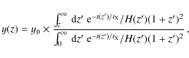
In Fig. 1, we show the spectral distortion, $\Delta I_\nu$ , including 2 shells in our computations for different transitions as a function of redshift. It was assumed that energy was released in a single injection at z_i=50 000, producing y=10^-5. All shown curves were computed using the $\delta$ -function approximation for the line-profiles (Kholupenko et al. 2005; Rubiño-Martín et al. 2006; Wong et al. 2006), in which the distortion is given by $\Delta I_{ij}(z)= \frac{hc}{4\pi}~\Delta R_{ij}(z)/H(z)[1+z]^3$ , where $\Delta R_{ij}$ is the net rate of the transition $i\rightarrow j$ . This approximation is insufficient when one is interested in computing the true spectral distortions in frequency space, since for the free-bound contribution the recombinational lines are very broad (e.g., see Chluba & Sunyaev 2006). In addition, one should include the line-broadening due to electron scattering as explained in Appendix A.4 and the correct mapping from $z\rightarrow \nu$ .

We note that in the $\delta$ -function approximation for the line profiles one has $\Delta I_{ij}(z)\equiv f(z)~\Delta R_{ij}(z)$ , where f(z) depends only on redshift and not on the considered transition. Therefore, considering $\Delta I_{ij}(z)$ is a convenient way of studying the redshift dependence of the net rates between different levels.

$\begin{figure} \par\includegraphics[width=8.8cm,clip]{eps/9840f1a.eps}\vspace*{3mm} \includegraphics[width=8.8cm,clip]{eps/9840f1b.eps} \end{figure}$

Figure 1:

Spectral distortion, $\Delta I_\nu$ , including 2 shells into our computations for different transitions as a function of redshift and for y=10^-5. All shown curves were computed using the $\delta$ -function approximation for the intensity. The upper panel shows the results for hydrogen, the lower those for He II. In both cases the analytic approximation for the Lyman- $\alpha$ line based on Eqs. (B.2) and (B.7), and including the escape probabilities in the Lyman- $\alpha$ line and Lyman-continuum, are also shown. Note that in the chosen representation the Lyman- $\alpha$ line and Balmer-continuum coincide at high redshifts. This is because their photons are emitted simultaneously and in equal amount as parts of the same atomic loop ( ${\rm c}\rightarrow {\rm 2p}\rightarrow {\rm 1s}\rightarrow {\rm c}$ ).

Open with DEXTER

Looking at Fig. 1, one can see that prior to the recombination epoch of the considered species one can find pre-recombinational emission and absorption in the Lyman- and Balmer-continuum, and the Lyman- $\alpha$ line, which would be completely absent for y=0. As expected, during the pre-recombinational epochs the 2s-1s-two-photon transition is not important. This is because the 2s-1s transition is simply unable to compete with the ${\sim}10^8$ times faster Lyman- $\alpha$ transition while the latter remains optically thin.

Summing the spectral distortions caused by the continua, one finds cancellation of the redshift-dependent emission at a level close to our numerical accuracy (relative accuracy ${\la}10^{-4}$ for the spectrum). This is expected because of electron number conservation: in the pre-recombinational epoch the overall ionization state of the plasma is not affected significantly by the small deviations of the background radiation from full equilibrium. Therefore, all electrons that enter an atomic species will leave it again, in general via another route to the continuum. This implies that $\sum_i \Delta R_{{\rm c}i}=0$ , which is a general property of the solution in the pre-recombinational epoch. This can also be concluded from Fig. 1, since in the $\delta$ -function representation the Balmer-continuum line prior to the recombination epoch cancels the Lyman-continuum line at each redshift.

If we look at the Lyman- and Balmer-continuum in the case of hydrogen, we can see that at redshifts $z\ga 30~000$ , electrons enter by the Lyman-continuum, and leave by the Balmer-continuum, while in the redshift range $2000\la z\la 30~000$ the opposite is true (see Sect. 5.1.1 for a detailed explanation). As expected, for $z\ga 2000$ the Lyman- $\alpha$ transition exactly follows the Balmer-continuum, since every electron that enters the 2p-state and then reaches the ground level, also must pass through the Lyman- $\alpha$ transition. Using the analytic solution for the Lyman- $\alpha$ line given in the Appendix B, we find excellent agreement with the numerical results until the true recombination epoch is entered at $z\la 2000$ .

In the case of He II for the considered range of redshifts, the pre-recombinational emission ( $z\ga 7000$ ) is always generated in the loop ${\rm c}\rightarrow {\rm 2p}\rightarrow {\rm 1s}\rightarrow {\rm c}$ . We again find excellent agreement with the analytic solution for the Lyman- $\alpha$ line. We note that for He II the total emission in the pre-recombinational epoch is much higher than in the recombination epoch at $z\sim 6000$ (see discussion in Sect. 4). The height of the maximum is even comparable to the H I Lyman- $\alpha$ line.

As one can see in Fig. 1, at high redshift all transitions become weaker. This because the rest-frame frequencies of all lines are in the Rayleigh-Jeans part of the CMB spectrum, where the effective chemical potential of the y-distortion (see Sect. 2.1) decreases as $\mu(x)\approx 2x~y$ . This implies that at higher redshift all transitions are more and more within a pure blackbody ambient radiation field. On the other hand, the effective chemical potential increases towards lower redshift, so that also the strength of the transitions increases. However, at $z\la 3000$ in the case of hydrogen, and $z\la 11~000$ for He II, the escape probability in the Lyman-continuum (see Appendix A.1 and Eq. (B.3) for quantitative estimates) begins to decrease significantly, so that the pre-recombinational transitions cease. For a 2-shell atom this is because, the only loop that can operate is via the Lyman-continuum. The maximum in the pre-recombinational Lyman- $\alpha$ line forms because of this rather sharp transition to the optically thick region of the Lyman-continuum (see also Sect. 5.1.1 for more details).

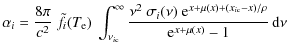
5.1.1 Analytic description of the pre-recombinational Lyman- $\alpha$ line

One can understand the behavior of the numerical solution for the spectral distortions in more detail using our analytic description of the Lyman- $\alpha$ line given in Appendix B.

In Fig. 2, we show the comparison of different analytic approximations with the full numerical result. The curves labeled ``analytic Ia'' (dotted line) and ``analytic Ib'' (boxes) are both based on the formulae in Eqs. (B.2) and (B.7). In their derivation, we assumed that the population of the 2p-state evolves under quasi-stationary conditions, where the free electron fraction and proton number density are given by the R ECFAST-solution. For the approximation ``analytic Ia'', we did not include the escape probabilities in the H I Lyman- $\alpha$ line and H I Lyman-continuum, while the approximation ``analytic Ib'' also includes the escape probabilities described in Appendix B.1.1. A comparison of these curves indicates that for the shape of the distortion at $z\la 3000$ , the escape probabilities are very important. However, although at this redshift the Sobolev optical depth in the H I Lyman- $\alpha$ line is roughly a factor of 14 higher than the optical depth in the H I Lyman-continuum, the derivation of Eq. (B.8) shows that the H I Lyman- $\alpha$ escape probability plays only a secondary role in the pre-recombinational era.

Given the formulae in Appendix B.1.2, the spectral distortion can be written in the form $\Delta I_\nu(z)=F(z)\times \Delta$ . The factor F(z) describes the normalization of the line (see Eq. (B.8)), also including the effect of the escape probabilities in the H I Lyman- $\alpha$ line and continuum. One does not expect a strong change in the line shape when using simple equilibrium values in its evaluation. For simplicity, we assume below that F is given by Eq. (B.10), which should be accurate to a level of ${\sim}20\%$ for the considered redshift range.

The term, $\Delta$ , which is related to the imbalance of emission and absorption, should allow us to understand when and why the Lyman- $\alpha$ line becomes negative. In the most radical approximation (see Appendix B.1.2 for details), one can use $\Delta\approx \mu_{21}+\mu_{\rm 2~pc}-\mu_{\rm 1~sc}$ , as derived in Eq. (B.14b), so that we obtain the curve labeled ``analytic II''. One can clearly see that this approximation represents the global behavior, but fails to explain the Lyman- $\alpha$ absorption at $z\ga 30~000$ . For this approximation, the Lyman- $\alpha$ line should always be in emission, even at high redshift, since with $\mu(x)\approx 2yx[1-x^2/12]$ in the limit of small x, we have $\Delta\approx 3~y~x^3_{\rm 1sc}/32>0$ . This approximation indicates that to lowest order the main reason for emission in the Lyman- $\alpha$ line is the deviation of the effective chemical potential from zero at the Lyman- $\alpha$ resonance, and the Lyman- and Balmer-continuum frequency.

$\begin{figure} \par\includegraphics[width=8.8cm,clip]{eps/9840f2.eps} \end{figure}$	Figure 2: Analytic representation of the pre-recombinational H I Lyman- $\alpha$ spectral distortions for the 2 shell atom and y=10^-5. See text for explanations. Note that at $z \protect\ga 3000$ the curves labeled ``analytic Ia'' and ``analytic Ib'' coincide.
Open with DEXTER

$\begin{figure} \par\includegraphics[width=8.8cm,clip]{eps/9840f3a.eps}\vspace*{3mm} \includegraphics[width=8.8cm,clip]{eps/9840f3b.eps} \end{figure}$	Figure 3: Spectral distortion, $\Delta I_\nu$ , including 3 shells into our computations for different transitions as a function of redshift and for y=10^-5. For all shown curves we used the $\delta$ -function approximation to compute the intensity. The upper panel shows the results for hydrogen, the lower those for He II.
Open with DEXTER

If we also account for the higher order terms of the line imbalance $\Delta$ according to Eq. (B.16a), then we obtain the curve labeled ``analytic III'', which is close to the full solution and also reproduces its high redshift behavior, starting at a slightly higher redshift ( $z\sim 40~000$ instead of $z\sim 30~000$ ). This is mainly caused by the approximations in the integrals (B.15) over the photoionization cross-sections (in particular M_-1). However, if one evaluates these integrals more accurately, one does not recover the full solution exactly, since the free-bound Gaunt-factors are neglected; only when these factors are included and we evaluate the factor F correctly can we again obtain the full numerical result.

5.2 The 3-shell atom

If one considers 3 shells, the situation becomes more complicated, since more loops connecting to the continuum are possible. Looking at Fig. 3, again we find that the sum over all transition in the continua vanishes at redshifts prior to the true recombination epoch of the considered species. At $z\la 3000$ in the case of hydrogen and $z\la 11~000$ for He II, the escape probability in the Lyman-continuum becomes small. For 2 shells, this stopped the pre-recombinational emission until the true recombination epoch of the considered atomic species was entered (see Fig. 1). However, for 3 shells electrons can leave the 1s-level via the Lyman- $\beta$ transition, and reach the continuum through the Balmer-continuum. For both hydrogen and He II, one can also see that the emission in the Lyman- $\alpha$ line stops completely when the Lyman-continuum is fully blocked. In this situation, only the loop ${\rm c}\rightarrow {\rm 3}\rightarrow 2 \rightarrow {\rm c}$ via the Balmer-continuum operates. Only when the main recombinational epoch of the considered species is entered, is the Lyman- $\alpha$ line reactivated.

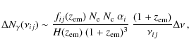
$\begin{figure} \par\includegraphics[width=4.3cm,clip]{eps/9840f4a.eps}\hspace*{3mm} \includegraphics[width=4.3cm,clip]{eps/9840f4b.eps} \end{figure}$	Figure 4: Sketch of the main atomic loops for hydrogen and He II when including 3 shells. The left panel shows the loops for transitions that are terminating in the Lyman-continuum. The right panel shows the case, when the Lyman-continuum is completely blocked, and unbalanced transitions are terminating in the Balmer-continuum instead.
Open with DEXTER

In Fig. 4, we sketch the main atomic loops in hydrogen and He II when including 3 shells. For y=10^-5, in the case of hydrogen the illustrated Lyman-continuum loops work in the redshift range $2000\la z\la 30~000$ , while the Balmer-continuum loop works for $1600\la z \la 2000$ . In the case of He II, one finds that $8000\la z \la 1.2 \times 10^{5}$ and $6200\la z \la 8000$ for the Lyman- and Balmer-continuum loops, respectively. It is clear that in every closed loop, one energetic photons is destroyed and at least two photons are generated at lower frequencies. Including more shells will open the possibility of generating more photons per loop, simply because electrons can enter through highly excited levels and then preferentially cascade to the lowest shells via several intermediate levels, leaving the atomic species taking the fastest available route back to the continuum. We discuss this situation below in more detail (see Sect. 5.3.1).

Figures 1 and 3 both show that the pre-recombinational lines are emitted in a typical redshift range $\Delta z/z\sim 1$ , while the signals from the considered recombinational epoch are released within $\Delta z/z\sim 0.1{-}0.2$ . For the pre-recombinational signal, the expected line-width is $\Delta\nu/\nu\sim 0.6{-}0.7$ . However, the overlap of several lines, especially at frequencies where emission and absorption features nearly coincide, and the asymmetry of the pre-recombinational line profiles, still leads to more narrow spectral features with $\Delta\nu/\nu\sim 0.1{-}0.3$ (see Sect. 5.3, Fig. 6).

We also note that in all cases the true recombination epoch is not affected significantly by the small y-distortion in the ambient photon field. There the deviations from Saha-equilibrium because of the recombination dynamics dominate over those directly related to the spectral distortion, and in particular the changes in the ionization history are tiny.

$\begin{figure} \par\includegraphics[width=8.8cm,clip]{eps/9840f5a.eps}\includegr... ...eps/9840f5e.eps}\includegraphics[width=8.8cm,clip]{eps/9840f5f.eps} \end{figure}$

Figure 5:

Contributions to the H I ( left panels) and He II ( right panels) recombination spectrum for different values of the initial y-parameter. Energy injection was assumed to occur at $z_i=4 \times 10^{4}$ . In each column the upper panel shows the bound-bound signal, the middle the free-bound signal, and the lower panel the sum of both. Thin red lines represent the overall negative parts of the signals. Note that the 2s-1s-two-photon decay contribution is not shown, since it does not lead to any significant pre-recombinational signal.

Open with DEXTER

$\begin{figure} \par\includegraphics[width=8.8cm,clip]{eps/9840f6a.eps}\includegr... ...eps/9840f6e.eps}\includegraphics[width=8.8cm,clip]{eps/9840f6f.eps} \end{figure}$

Figure 6:

Main contributions to the H I ( left panels) and He II ( right panels) spectral distortion at different frequencies for energy injection at z_i=40 000 and y=10^-5. We have also marked those peaks coming (mainly) from the recombination epoch (``rec'') and from the pre-recombination epoch (``pre'') of the considered atomic species. Note that the 2s-1s-two-photon decay contribution is not shown, since it does not lead to any significant pre-recombinational signal.

Open with DEXTER

5.3 The 25-shell atom

In this section, we discuss the results for our 25-shell computations. Given the large amount of transitions, it is more efficient to look directly at the spectral distortion as a function of frequency. However, following the approach of Sect. 5.1, we checked that the basic properties of the first few lines and continua as a function of redshift qualitatively do not change in comparison to the previous cases. In particular, only the Lyman- and Balmer-continuum become strongly negative, again for similar redshift ranges as for 2 or 3 shells. In overall absorption, the other continua (n>2) play no important role, although about 10% of all loops do end there (see Sect. 5.3.1 for more details).

We note that for the spectral distortion now the impact of electron scattering must be considered and the free-bound contribution must be computed using the full differential, photoionization cross-section (see Appendix A.4).

5.3.1 Dependence of the distortion on the value of y

In Fig. 5, we show the contributions to the recombination spectrum for different values of the initial y-parameter. In addition, Fig. 6 shows some of the main contributions to the total hydrogen and He II spectral distortion in more detail.

Bound-bound transitions

Focusing first on the contributions of bound-bound transitions, one can see that the standard recombination signal due to hydrogen is not strongly affected when y=10^-7, whereas the helium signal already changed notably. Increasing the value of y in both cases leads to an increase in the overall amplitude of the distortion at low frequencies, and a large rise in the emission and variability at $\nu\ga 100$ GHz. For H I at low frequencies, the level of the signal increased roughly by a factor of 5 when increasing the value of y from 0 to 10^-5, while for He II the increase is about a factor of 40. This indicates that in the pre-recombinational epoch He II indeed behaves in a way similar to hydrogen, but with an amplification ${\sim}8$ (see Sect. 4).

At high frequencies, a strong emission-absorption feature appears in the range $\nu\sim 500{-}1600$ GHz, which is completely absent for y=0. For y=10^-5 from peak to peak, this feature exceeds the normal Lyman- $\alpha$ distortion (close to $\nu\sim1750$ GHz for H I and $\nu\sim1680$ GHz for He II) by a factor of ${\sim}5$ for H I, and about 30 for He II. The absorption part is caused mainly by the pre-recombinational Lyman- $\beta$ , - $\gamma$ , and - $\delta$ transitions, while the emission part is dominated by the pre-recombinational emission in the Lyman- $\alpha$ line (also see Fig. 6 for more detail).

We note that in the case of He II most of the recombinational Lyman- $\alpha$ emission ( $\nu\sim1750$ GHz) is completely wiped out by the pre-recombinational absorption in the higher Lyman-series, while for H I only a small part of the Lyman- $\alpha$ low frequency wing is affected. This is possible only because the pre-recombinational emission in the He II Lyman-series is so strongly enhanced, compared to the signal produced during the recombinational epoch.

Free-bound transitions

Considering the free-bound contributions, one can again see that the hydrogen signal changes much less with increasing value of y than in the case of He II. In both cases, the variability in the free-bound signal decreases at low frequencies, while at high frequencies a strong and broad absorption feature appears, which is mainly due to the Lyman-continuum. For y=10^-5, this absorption feature even completely erases the Balmer-continuum contribution appearing during the true recombination epoch of the considered species. It is 2 times stronger than the H I Lyman- $\alpha$ line from the recombination epoch, and in the case of He II it exceeds the normal He II Lyman- $\alpha$ line by more than one order of magnitude.

However, apart from the absorption feature at high frequencies the free-bound contribution becomes practically featureless when reaching y=10^-5. This is because of the strong overlap of different lines from the high redshift part, since the characteristic width of the recombinational emission increases as $\Delta\nu/\nu\sim kT_{\rm e}/h \nu_{i\rm c}$ (see middle panels in Fig. 5). In addition, the photons are released in a broader range of redshifts (see Sects. 5.1 and 5.2), leading to a decrease in the contrast between the spectral features from the recombinational epoch.

Total distortion

In the total spectra (see lower panels in Fig. 5), one can also clearly see a strong absorption feature at high frequencies, which is mainly associated with the Lyman-continuum and Lyman-series for n>2 (see Fig. 6 also). For y=10^-5, in the case of hydrogen it exceeds the Lyman- $\alpha$ line from recombination ( $\nu\sim1750$ GHz) by a factor of ${\sim}4$ at $\nu\sim 1250$ GHz, while for He II it is even stronger by a factor of ${\sim}20$ , reaching ${\sim}80\%$ of the corresponding hydrogen feature. Checking the level of emission at low frequencies, as expected (see Sect. 4), one can find that He II indeed contributes about 2/3 to the total level of emission.

As illustrated in the upper panels of Fig. 6, the emission-absorption feature at high frequencies is caused by the overlap between the pre-recombinational Lyman- $\alpha$ line (emission) and the combination of the higher pre-recombinational Lyman-series and Lyman-continuum (absorption). At intermediate frequencies (middle panels), the main spectral features are due to the Balmer- $\alpha$ , the pre-recombinational Balmer-series from n>3, and the Paschen- $\alpha$ transition, with some additional broad contributions to the overall amplitude of the bump originating in higher continua.

The lower panels of Fig. 6 show, as an example, the separate contributions to the bound-bound series for the 10th shell. One can notice that for hydrogen the recombinational and pre-recombinational emission are of similar amplitude, while for He II the pre-recombinational signal is more than one order of magnitude stronger (see Sect. 4 for an explanation). In both cases, the pre-recombinational emission is much broader than the recombinational signal, again mainly due to the time-dependence of the photon emission process (see Sects. 5.1 and 5.2), but to some extent also because of electron scattering.

Number of additional photons and loops

Using the free-bound spectrum, one can also estimate the effective number of loops, ${\mathcal{N}_{\rm loop}}$ , involved in the production of all photons seen as additional CMB spectral distortion. The easiest way to compute this number is to consider the free-bound spectrum of each level using the $\delta$ -function approximation. In this way, one avoids the overlap between the emission and absorption contributions at different redshifts, which would lead to a small underestimation of ${\mathcal{N}_{\rm loop}}$ . In the case of full equilibrium, one should find that ${\mathcal{N}_{\rm loop}}=0$ .

By computing the number of photons that can be seen as overall free-bound emission, one obtains the number of times an electron has entered an uncompensated loop via the considered level. On the other hand, by computing the number of photons that can be seen as overall bound-free absorption, one can determine the number of times that an uncompensated transition ended at that level. By evaluating the sum over the number of photons that can be seen as overall free-bound emission from all levels, one should find ${\mathcal{N}_{\rm loop}}+1$ photons per nucleus. Similarly, the total number of photons absorbed in all bound-free transitions should be ${\mathcal{N}_{\rm loop}}$ photons per nucleus. The difference of ${\sim}1\gamma$ per nucleus is due the fact that at the end of the recombinational epoch of each atomic species practically all electrons have been captured, without returning to the continuum afterwards. In a similar way, one can also identify the partial contribution of each continuum.

In Table 1, we provide a few examples, comparing also with the number of photons emitted for y=0. One can see that the effective number of loops per nucleus varies roughly in proportion to the values of y, i.e., ${\mathcal{N}^{H {\sc i}}_{\rm loop}}\sim 3.3$ $\times$ [y/10^-5] and ${\mathcal{N}^{He {\sc ii}}_{\rm loop}}\sim 31$ $\times$ [y/10^-5]. If one considers a lower injection redshift, the proportionality constant should decrease, since the loops will be active over a shorter period. When also including more shells, ${\mathcal{N}_{\rm loop}}$ should increase because there are more channels through which the electrons can enter the atoms. Furthermore, the effective number of loops per nucleus is about one order of magnitude larger for He II than for hydrogen. As explained in Sect. 4, this is caused by the amplification of transitions for hydrogenic helium at high redshift.

When comparing with the number of photons absorbed in the Lyman-continuum, one can also see that in practically all shown cases ${\sim}90\%$ of all loops should end there. By computing this more carefully for hydrogen assuming y=10^-5, we found that ${\sim} 85\%$ of the pre-recombinational loops end in the Lyman-continuum, about $4.2\%$ in the Balmer-continuum, ${\sim}0.4\%$ in the Paschen-continuum, and the remaining ${\sim} 10.4\%$ is distributed more or less evenly over all the other continua, with no strong drop toward higher shells. For helium, we found similar numbers.

Table 1: Approximate number of photons and loops per nucleus of the considered species for $z_i=4 \times 10^{4}$ and different values of y.

$\begin{figure} \par\includegraphics[width=8.8cm,clip]{eps/9840f7a.eps}\vspace*{3mm} \includegraphics[width=8.8cm,clip]{eps/9840f7b.eps} \end{figure}$	Figure 7: H I ( upper panel) and He II ( lower panel) recombination spectra for different energy injection redshifts.
Open with DEXTER

$\begin{figure} \par\includegraphics[width=8.8cm,clip]{eps/9840f8a.eps}\vspace*{3mm} \includegraphics[width=8.8cm,clip]{eps/9840f8b.eps} \end{figure}$	Figure 8: Total H I + He II recombination spectra for different energy injection redshifts. The upper panel shows details of the spectrum at low, the lower at high frequencies.
Open with DEXTER

If we considered the total number of photons per nucleus emitted in the bound-bound transitions and subtracted the number of photons emitted for y=0, we were able to estimate the loop-efficiency, $\epsilon_{\rm loop}$ , or number of bound-bound photons generated per loop prior to the recombination epoch. For hydrogen, one finds $\epsilon_{\rm loop}\sim 2.9{-}3.0$ , while for He II one has $\epsilon_{\rm loop}\sim 3.2{-}3.3$ . Similarly, one obtains a loop efficiency of $\epsilon_{\rm loop}\sim 1.7{-}1.8$ for both the H I and He II Lyman- $\alpha$ lines. As expected these numbers are rather independent of the value of y, since they should reflect an atomic property. They should also be rather independent of the injection redshift, which mainly affects the total number of loops and thereby the total number of emitted photons. However, the loop efficiency should still increase when including more shells in the computation.

$\begin{figure} \par\includegraphics[width=8.8cm,clip]{eps/9840f9a.eps}\includegr... ...eps/9840f9c.eps}\includegraphics[width=8.8cm,clip]{eps/9840f9d.eps} \end{figure}$

Figure 9:

Comparison of the variable component in the H I + He II bound-bound and free-bound recombination spectra for single energy injection at different redshifts. In all cases the computations were performed including 25 shells and y=10^-5. The blue dashed curve in all panel shows the variability in the normal H I + He II recombination spectrum (equivalent to energy injection below $z\sim 800$ or y=0) for comparison.

Open with DEXTER

5.3.2 Dependence of the distortion on the redshift of energy injection

To understand how the pre-recombinational emission depends on the redshift at which the energy was released, in Fig. 7 we show a compilation of different cases for the total H I and He II signal. In Fig. 8, we also present the sum of both in more detail.

Features at high frequencies

For all shown cases, the absolute changes in the curves are strongest at high frequencies ( $\nu\ga 100$ GHz). One can also identify a rather broad bump at $100~{\rm GHz}\la\nu\la 400~{\rm GHz}$ , followed by an emission-absorption feature in the frequency range $500~{\rm GHz}\la\nu\la 1600~{\rm GHz}$ . In particular the strength and position of this emission-absorption feature depends strongly on the redshift of energy injection.

For the broad high-frequency signature, it is more important that the variability itself varies, rather than the overall amplitude increases. For example, in the frequency range $100~{\rm GHz}\la\nu\la 400~{\rm GHz}$ , the normal recombinational signal has ${\sim}2$ spectral features, while for injection at $z_i\sim 4000$ approximately 4 features are visible, which in this case only come from hydrogen because at $z\sim 4000$ He II is already completely recombined. We also note that neutral helium should add some signal, which was not included here. Nevertheless, we expect that this contribution is not strongly amplified as in the case of He II (see Sect. 4), and hence should not increase the total signal by more than $10{-}20\%$ .

Variability at low frequencies

Focusing on the spectral distortions at low frequencies, the overall level of the distortion in general increases for higher redshifts of energy release. However, there is also some change in the variability of the spectral distortions. To study this variability in more detail, in each case we performed a smooth spline fit of the total H I + He II recombination spectrum and then subtracted this curve from the total spectrum. The remaining modulation of the CMB intensity was then converted into variations in the CMB brightness temperature using the relation $\Delta T/T_0 \approx \Delta I / B_{\nu}$ , where $B_\nu$ is the blackbody intensity at temperature T₀=2.725 K.

Figure 9 shows the results of this procedure in several cases. It is most striking that the amplitude of the variable component decreases with increasing energy injection redshift. This can be understood as follows: we have seen in Sects. 5.1 and 5.2 that for very early energy injection most of the pre-recombinational emission is expected to be produced at $z\sim 3000$ for hydrogen, and $z\sim 11~000$ for helium, (i.e., the redshifts at which the Lyman-continuum of the considered atomic species becomes optically thick) with a typical line-width $\Delta\nu/\nu\sim 1$ . In this case, the total variability of the signal is mainly due to the non-trivial superposition of many broad neighboring spectral features. Most importantly, little variability will be added by the high redshift wing of the pre-recombinational lines and in particular the beginning of the injection process. This is because (i) at high z the emission is much smaller (cf. Figs. 1 and 3); and (ii) electron scattering broadens lines significantly, smoothing any broad feature even more (see Appendix A.4).

On the other hand, when the energy injection occurs at lower redshift, this increases the variability of the signal because (i) electron scattering in the case of single momentary energy release does not smooth the step-like feature due to the beginning of the injection process as strongly; and (ii) the total emission amplitude and hence the step-like feature increases (see Figs. 1 and 3). When the injection occurs close to the redshift at which the Lyman-continuum is optically thick (see Sect. 5.1), i.e., where the pre-recombinational emission has an extremum, this should produce a strong increase in the variability. On the other hand, for energy injection well before this epoch the atomic transitions produce an increase in the overall amplitude of the distortions rather than the variability.

This can also be seen in Fig. 9, where for z_i=4000 the variable component is ${\sim}3{-}8$ times larger than the normal recombinational signal with a peak-to-peak amplitude of ${\sim}50{-}70$ nK instead of ${\sim}10{-}15$ nK at frequencies around ${\sim}1.5$ GHz. Even for $z_i\ga 15~000$ , the amplitude of the variable component is still 1.5-2 times larger than in the case of standard recombination, but it practically does not change anymore when going to higher injection redshifts. For $z_i\sim 11~000$ , one expects a similarly strong increase in the variability as for $z_i\sim 4000$ , but this time due to He II. In addition to the change in amplitude of the variable component, in all cases the signal is shifted with respect to the normal recombinational signal. These shifts should also make it easier to distinguish between the spectral signatures from pre-recombinational energy release and those produced by normal recombination.

It is important to mention that the total amplitude of the variable component should still increase when more shells are included in the computation. As shown in Chluba et al. (2007a), for y=0 in particular the overall level of recombinational emission at low frequencies depends strongly on the completeness of the atomic model. Similarly, the variability in the recombination spectrum changes. This is illustrated in Fig. 10, where we compare the variability in the H I + He II recombination spectrum for 25 shells (y=0), with that obtained in our 100-shell computations (Chluba et al. 2007a; Rubiño-Martín et al. 2008). As one can see, at low frequencies ( $\nu\sim 1{-}3$ GHz) the amplitude of the variable component increases by more than a factor of 2 when 100 shells are included, reaching a peak-to-peak amplitude of ${\sim}30$ nK. This is due to the fact that for a more complete atomic model additional electrons are able to pass through a particular transition between highly excited states.

$\begin{figure} \par\includegraphics[width=8.8cm,clip]{eps/9840f10.eps} \end{figure}$	Figure 10: Comparison of the variable component in the standard (y=0) H I + He II bound-bound and free-bound recombination spectrum for $n_{\rm max}=100$ and 25.
Open with DEXTER

$\begin{figure} \par\includegraphics[width=8.8cm,clip]{eps/9840f11a.eps}\vspace*{3mm} \includegraphics[width=8.8cm,clip]{eps/9840f11b.eps} \end{figure}$	Figure 11: Comparison of the variable component in the H I + He II bound-bound and free-bound recombination spectra for single energy injection (black solid curves) and energy injection due to long-lived decaying particles with different lifetimes (red dashed-dotted curves). In all cases the computations were performed including 25 shells and a maximal y-parameter y=10^-5.
Open with DEXTER

5.3.3 Dependence of the distortion on the energy injection history

Until now we have only considered cases of single momentary energy injection. However, physically this may not be very realistic, since most of the possible injection mechanisms release energy over a broader range of redshifts. The discussion in Sect. 5.3.2 has also shown that for single injection a large part of the variability can be attributed to the onset of the energy release. Therefore it is important to investigate the potential signatures of other injection mechanisms.

For the signals under discussion, long-lived, decaying particles are the most interesting. In Sect. 2.1.1, we have given some simplified analytic description of this problem. In Fig. 11, we show the variable component for the CMB spectral distortion due to the presence of hydrogen and He II at low frequencies, for both single injection and energy release from long-lived decaying particles. For $z_{\rm X}=4000$ , it is clear that the variability is significantly smaller than in the case of single energy injection. This is because the onset of the atomic transitions is much more gradual than in the case of single injection. However, one should mention that for energy injection due to decaying particles the effective y-parameter at z=4000 remains only ${\sim}1/3$ of its maximal value, so that the level of variability cannot be compared directly with the case of single energy injection. Nevertheless, the structure of the variable component still depends non-trivially on the effective decay redshift, so that one in principle should be able to distinguish between the different injection scenarios.

Similarly, one could consider the case of annihilating particles. However, here energy is effectively released at higher redshift and also over a much broader redshift interval. In this case, one has to follow the evolution in the CMB spectrum caused by this heating mechanism from an initial $\mu$ -type distortion to a partial y-type distortion in more detail. One can also expect that the redistribution of photons via electron scattering will become much more important (see Appendix A.4), and that the free-free process will strongly alter the number of photons emitted via atomic transitions (see Appendix A.5). In addition, collisional processes may become significant, in particular those leading to transitions among different bound-bound levels, or to the continuum, since they are not associated with the emission of photons. This problem will be considered in a future work.

6 Discussion and conclusions

In the previous sections, we have shown in detail how intrinsic y-type CMB spectral distortions modify the radiation released by atomic transitions in primordial hydrogen and He II at high redshift. We presented the results of numerical computations including 25 atomic shells for both H I and He II, and discussed the contributions of several individual transitions in detail (e.g., see Fig. 6), by also taking the broadening of lines due to electron scattering into account. As examples, we investigated the case of instantaneous energy release (Sect. 5.3.2) and exponential energy release (Sect. 5.3.3) due to long-lived, decaying particles, separately.

Our computations indecated that several additional photons are released during the pre-recombinational epoch, which in terms of number can strongly exceed those from the recombinational epoch (see Sect. 5.3.1). The number of loops per nucleus scales roughly in proportion to the values of y, i.e., ${\mathcal{N}^{H {\sc i}}_{\rm loop}}\sim 3.3$ $\times$ [y/10^-5] and ${\mathcal{N}^{He {\sc ii}}_{\rm loop}}\sim 31$ $\times$ [y/10^-5] for hydrogen and He II, respectively, where about 3 photons per loop are effectively emitted in the bound-bound transition.

Because of the non-trivial overlap of broad neighboring pre-recombinational lines (from bound-bound and free-bound transitions), rather narrow ( $\Delta\nu/\nu\sim 0.1{-}0.3$ ) spectral features appear on top of a broad continuum, which both in shape and amplitude depend on the time-dependence of the energy injection process and the value of the intrinsic y-type CMB distortion. At high frequencies ( $\nu\sim 500{-}1600$ GHz), an emission-absorption feature forms, which is completely absent for y=0, and is mainly due to the superposition of pre-recombinational emission in the Lyman- $\alpha$ line, and the higher Lyman-series and Lyman continuum.

Looking at Fig. 12, it becomes clear that this absorption feature (close to $\nu\sim 1400$ GHz) in all shown cases even exceeds the intrinsic y-distortion. For y=10^-5, it even reaches ${\sim}10\%$ of the CMB blackbody intensity. Unfortunately, it appears in the far Wien-tail of the CMB spectrum, where the cosmic infrared forming galaxies is dominant (Lagache et al. 2005; Fixsen et al. 1998). Still one may hope to be able to extract such spectral features in the future.

$\begin{figure} \par\includegraphics[width=8.8cm,clip]{eps/9840f12.eps} \end{figure}$	Figure 12: Spectral distortions relative to the CMB blackbody spectrum, $B_\nu$ . The thin blue curves show the absolute value of a y-type distortion. At low frequencies we indicate the expected level of emission when including more shells in our computations.
Open with DEXTER

One should emphasize that all the discussed additional pre-recombinational spectral distortions are in general small in comparison to the intrinsic y-distortion. As Fig. 12 shows, the amplitude of the additional distortions is typically well below 1% of the CMB y-distortion. However, at low frequencies ( $\nu\sim 1$ GHz) the additional distortions should reach ${\sim}10\%$ of the intrinsic y-distortion, and at even lower frequency may also exceed it. But in this context, it is more important that due to the processes discussed here new narrow spectral features appear, of an unique variability (e.g. see Fig. 9), even stronger than that of the recombinational lines from standard recombination (y=0). This variability is very hard to mimic by any astrophysical foreground or systematic problem with the instruments. As emphasized earlier for the cosmological recombination spectrum (Sunyaev & Chluba 2007,2008), this may allow us to measure them differentially, also making use of the fact that the same signal is coming from practically all directions on the sky. For intrinsic y-distortions, direct differential measurements are much harder, since its spectrum is so broad. Furthermore, as pointed out in the introduction, by measuring the narrow spectral features under discussion one could in principle distinguish between pre- and post-recombinational energy release, an observation that cannot be easily achieved by measuring directly the average y-distortion of the CMB.

We also note that in addition to the average y-parameter one could include possible knowledge on the angular dependence of the CMB spectrum. The y-distortion from resolved SZ-clusters is a trivial example and their signals can certainly be removed. However, the contributions from the warm-hot-interstellar-medium should be more uniform and should vary at very different angular scales. The presence of halos of annihilating ( ${\propto}N_{\rm dm}^2$ ) or decaying ( ${\propto}N_{\rm dm}$ ) dark matter at high redshifts ( $z\ga 20$ ) will also lead to a slowly varying, angular-dependent, post-recombinational y-distortion. Because of their different dependencies on the dark matter number density $N_{\rm dm}$ , these contributions will influence different angular scales at different redshifts. This angular dependence in principle would provide another way to separate pre- and post-recombinational energy release. However, one should also consider that the pre-recombinational energy release may not be uniform, since for example, phase transitions in different parts of the Universe occur at different redshifts. This makes the problem more involved and a detailed analysis of this possibility is beyond the scope of this paper.

We have also pointed out that there is no principle difficulty in computing the spectral distortions due to pre-recombinational atomic transitions in H I and He II for more general energy injection histories, if required. In particular very early injection, involving $\mu$ -type distortions, may be interesting, since stimulated emission could strongly amplify the emission at low frequencies and hence the total number of emitted photons per atom. However, to treat this problem one has to follow the detailed evolution in the CMB spectral distortion produced by the injection process (see e.g. Hu & Silk 1993a). The effect of electron scattering on the distortions caused by the pre-recombinational atomic transitions, in particular because of the recoil effect, must also be treated more rigorously. Simple estimates also show (see Appendix A.5) that at low frequencies the modifications due to free-free absorption becomes significant. Furthermore, one must account for collisional processes, since they should become important at very high redshift, even for shells with low n.

An additional difficulty arises because at both very low and very high frequencies, the back-reaction of the pre-recombinational distortion on the ambient radiation field may not be negligible (see Fig. 12). This may also affect the details of the results presented here, although our main conclusions should not change. The inter-species feedback and reprocessing of photons (e.g. $\gamma_He {\sc ii}\rightarrow He {\sc i}$ and $\gamma_He {\sc }\rightarrow H {\sc i}$ ) may also produce some differences, close to the beginning of the pre-recombinational epochs of each atomic species. Furthermore, for more accurate predictions of the positions of the narrow features one should account for the background-induced, stimulated electron-scattering, which was discussed by Chluba & Sunyaev (2008a). We defer all of these problems to another paper.

Acknowledgements

The authors wish to thank J. A. Rubiño-Martín for useful discussions. We also wish to thank the referee for his comments and suggestions. In addition, we are grateful for discussions on experimental possibilities with J. E. Carlstrom, D. J. Fixsen, A. Kogut, L. Page, M. Pospieszalski, A. Readhead, E. J. Wollack and especially J. C. Mather. We would also like to thank J. Carlstrom and J. Ostriker for their comments and interest in the problem, and C. Thompson for additional discussion on superconducting strings. Also RS is very glad that he had the chance to work with Y. E Lyubarsky on the early ideas related to this problem.

Appendix A: Computational details

In this section, we outline the most important changes that had to be made to our multi-level code (Chluba et al. 2007a) to allow for an intrinsic y-type CMB spectral distortion. We also mention several approximations that can be used to ease the numerical integration of the coupled system of rate equations for the different populations of electrons in the energy levels of hydrogen and helium.

A.1 Formulation of the problem

Details about the formulation of the cosmological recombination problem for a pure blackbody CMB radiation field are given in Seager et al. (2000), Rubiño-Martín et al. (2006), and references therein. We shall use the same notation as in Rubiño-Martín et al. (2006). The main difference with respect to the standard recombination computation is caused by the possibility of a non-blackbody ambient radiation field, which affects the net bound-bound and free-bound rates as explained in Sect. 3. The temperature of the electrons in general is also no longer equal to the effective temperature of the photons, as we discuss below (see Sect. A.3). Since we consider only small intrinsic spectral distortions, all the modification to the solution for the level populations are rather small, and most of the differences will appear only as pre-recombinational emission due to atomic transitions, but with practically no net effect on the ionization history.

One additional modification is related to the Lyman-continuum. As was realized earlier (Peebles 1968; Zeldovich et al. 1968), during the recombination epochs photons cannot escape from the Lyman-continuum. However, at high redshift the number of neutral atoms is very small, so the Lyman-continuum becomes optically thin. To include the escape of photons in the Lyman-continuum, we follow the analytic description of Chluba & Sunyaev (2007), in which an approximation of the escape probability in the Lyman-continuum was given by

$\begin{displaymath}% P^{\rm Ly-c}_{\rm esc}(z)\approx \frac{1}{1+\tau^{\rm esc}_{\rm c}}, \end{displaymath}$

(A.1)

with $\tau^{\rm esc}_{\rm c}=\frac{c ~\sigma_{{\rm 1s c}}~N_{1s}}{H}\frac{k_{\rm B}T_{\rm e}}{h\nu_{\rm c}}$ . Here $\sigma_{{\rm 1s c}}$ is the threshold photoionization cross-section of the 1s-state, $N_{\rm 1s}$ is the number density of atoms in the ground state, and $\nu_{\rm c}$ is the threshold frequency. For a standard cosmology, the H I Lyman-continuum becomes optically thin above $z\sim 3000{-}4000$ , while for He II this occurs at $z\ga 12~000{-}16~000$ . As our computations show, it is crucial to include this process, since at high redshift almost all loops begin or terminate in the Lyman-continuum (see Sect. 5).

A.2 High redshift solution

At high redshift, well before the true recombination epoch of the considered atomic species, one can simplify the problem by realizing that the ionization degree does not change significantly. Although the inclusion of intrinsic CMB spectral distortion produces some small changes in the populations with respect to the Saha values, the total number of electrons captured by protons and helium nuclei is tiny compared to the total number of free electrons. Therefore, one can neglect the evolution equation for the electrons, until the true recombination epoch is entered. For H I, we used this simplification until $z\sim 3500$ , while for He II we follow the full system below $z\sim 20~000$ . Before we simply used the R ECFAST-solution for $N_{\rm e}$ (Seager et al. 1999,2000). In several different cases, we checked that these settings do not affect the spectra.

Furthermore, we note that at high redshift for n>2 we used the variable $\Delta N_i=N_i-N^{\rm 2s}_i$ instead of N_i, since $\Delta N_i/N_i$ becomes so small. Here $N^{\rm 2s}_i$ is the expected population of level i in Boltzmann-equilibrium relative to the 2s-level. We then changed back to the variable N_i at sufficiently low redshifts.

A.3 Recombination and photoionization rates

The computation of the photoionization and recombination rates for many levels is rather time-consuming. In an earlier version of our code (Chluba et al. 2007a), we tabulated the recombination rates for all levels before the actual computation and used detailed balance to infer the photoionization rates. This treatment is possible as long as the photon and electron temperature do not depart significantly from each other, and when the background spectrum is given by a blackbody. Here we now generalize this procedure accounting for the small difference between the electron and photon temperatures, in particular at low redshift ( $z\la 800$ ), and allowing for non-blackbody ambient photon distributions.

At high redshift ( $z \ga 3000$ ), the electron temperature is always equal to the Compton equilibrium temperature (Zeldovich & Sunyaev 1969):

$\begin{displaymath}% T_{\rm e}^{\rm eq}=\frac{k_{\rm B}T_{\gamma}}{h}~\frac{\int x^4 n_\gamma(x) {\,\rm d}x}{4 \int x^3 n_\gamma(x) {\,\rm d}x} \end{displaymath}$

(A.2)

within the given ambient radiation field. Because of the extremely high specific entropy of the Universe (there are ${\sim}1.6 \times 10^{9}$ photons per baryon), this temperature is reached on a much shorter timescale than the redistribution of photons via Compton scattering requires. For a $\mu$ -type distortion, $T_{\rm e}^{\rm eq}$ is always close to the effective photon temperature, whereas for a y-type distortion with $y\ll 1$ one has $T_{\rm e}\approx T_{\gamma}[1+5.4~y]$ (Illarionov & Syunyaev 1975a). This simplifies matters, since there is no need to solve the electron temperature evolution equation, and the photoionization and recombination rates can therefore be precalculated.

At redshifts below $z\sim 3000$ , we solve for the electron temperature accounting for the non-blackbody ambient radiation field. In this case, the photon temperature inside the term due to the Compton interaction must be replaced by $T_{\rm e}^{\rm eq}$ as given by Eq. (A.2), such that the temperature evolution equation reads

$\begin{displaymath}% \frac{\displaystyle\partial T_{\rm e}}{\displaystyle\partia... ... e}} ~[T_{\rm e}-T_{\rm e}^{\rm eq}]+\frac{2T_{\rm e}}{1+z}\,, \end{displaymath}$

(A.3)

where $\kappa_{\rm C}=4.91 \times 10^{-22}~{\rm s^{-1}~K^{-4}}$ .

Since for small intrinsic CMB spectral distortions, the correction to the solution for the temperature of the electrons is rather small, it is always possible to use the standard R ECFAST solution for $T_{\rm e}$ as a reference. Tabulating both the photoionization and recombination rates, and their first derivatives with respect to the ratio of the electron to photon temperature $\rho=T_{\rm e}/T_{\gamma}$ , it is possible to approximate the exact rates to high accuracy using first-order Taylor polynomials. To save memory, we only consider all these rates in some range of redshifts around the current point in the evolution and then update them from time to time. At high redshift, we typically used 200 points per decade in logarithmic spacing. At low redshift ( $z\la 5000$ ), we use 2 points per $\Delta z=1$ . Another improvement can be achieved by rescaling the reference solution for $T_{\rm e}$ with the true solution whenever the tabulated rates are updated. With these settings, we found excellent agreement with the full computation but at significantly lower computational cost.

A.4 Inclusion of electron scattering

As mentioned by Dubrovich & Stolyarov (1997) and shown in more detail by Rubiño-Martín et al. (2008), the broadening due to the scattering of photons by free electrons must be included in the computation of the He II recombination spectrum. Similarly, one has to account for this effect, when computing the spectral distortions arising from higher redshifts. Here we only consider redshifts $z\la 5 \times 10^{4}$ , and hence the electron scattering Compton-y-parameter

$\begin{displaymath}% {y_{\rm e}}(z)=\!\!\int_0^z\!\!\frac{kT_{\rm e}}{m_{\rm e}c... ... T}}{H(z')(1+z')}{\,\rm d}z'\approx4.8 \times 10^{-11}~[1+z]^2 \end{displaymath}$

(A.4)

is lower than ${\sim}0.12$ , so that the line-broadening due to the Doppler effect is significant ( $\Delta\nu/\nu\vert _{\rm Doppler}\sim 0.58$ ), but still moderate in comparison with the width of the quasi-continuous spectral features produced at high redshift (see Sects. 5.1 and 5.2). However, already at $z\la2.5 \times 10^{4}$ one has ${y_{\rm e}}\la 0.03$ , such that $\Delta\nu/\nu\vert _{\rm Doppler}\la 0.29$ .

Regarding the line-shifts caused by the recoil effect, one finds that they are not very important, since even for the H I Lyman-continuum one has $\Delta\nu/\nu\vert _{\rm recoil}\la -0.14$ at $z\la 5 \times 10^{4}$ . Although for the He II Lyman-continuum the shifts due to the recoil-effect is a factor of four higher, we shall not include it in our results. One therefore expects that at frequencies $\nu \ga 57$ GHz the presented distortions may still be modified due to this process, but we will consider this problem in a future paper.

For the bound-bound spectrum we follow the procedure described in Rubiño-Martín et al. (2008), where the resulting spectral distortion at observing frequency $\nu$ for one particular transition is given by (see also Zeldovich & Sunyaev 1969)

$\begin{displaymath}% \left.\Delta I_{ij}(\nu)\right\vert _{\rm Doppler}= \int\fr... ...{\rm e}})^2}{4{y_{\rm e}}}} ~\frac{{\,\rm d}\nu_0}{\nu_0}\cdot \end{displaymath}$

(A.5)

Here $\Delta I_{ij}(\nu_0)$ denotes the spectral distortion for the considered transition evaluated at frequency $\nu_0$ and computed without the inclusion of electron scattering (e.g., see Rubiño-Martín et al. 2006), but accounting for the non-blackbody ambient radiation field. We note that ${y_{\rm e}}(z)$ has to be calculated starting at the emission redshift ${z_{\rm em}}=\nu_{ij}/\nu_0-1$ , where $\nu_{ij}$ is the transition frequency.

For the spectral distortion resulting from the free-bound transitions, one in addition has to include the frequency-dependence of the photoionization cross-section. We shall neglect the line broadening because of electron scattering for the moment. Then, following Chluba & Sunyaev (2006) and using the definitions of Sect. 3.2, in the optically thin limit the spectral distortion of the CMB at observing frequency $\nu$ due to direct recombinations to level i is given by

$\displaystyle % \Delta I_{i\rm c}(\nu)$	=	$\displaystyle \frac{2~h\nu^3}{c^2}\! \int_{z_{\rm t}}^\infty n_\gamma(\nu_z, z)~\frac{c N_i~\sigma_{i}(\nu_z)}{H(z)(1+z)}$
		$\displaystyle \times~ \left[ \frac{N_{\rm e}~N_{\rm p}}{N_{i}} \tilde{f}_i(T_{\rm e})~{\rm e}^{x_z+\mu(x_z)+[x_{i\rm c}-x_z]/\rho} -1 \right]\! {\rm d} z,$	(A.6)

where $\nu_z=\nu~(1+z)$ , $1+z_{\rm t}=\nu_{i{\rm c}}/\nu$ and $x_z=h\nu_z/kT_{\gamma}\equiv h\nu/k T_0$ . Furthermore, $n_\gamma(\nu_z, z)$ denotes the intrinsic CMB occupation number at redshift z including the spectral distortion, evaluated at frequency $\nu_z$ . For the Lyman-continuum, one would in addition multiply the integrand of Eq. (A.6) by $P^{\rm Ly-c}_{\rm esc}(z)$ to obtain the approximate solution for the resulting distortion.

To include the broadening because of scattering by electrons, one has to solve the 2-dimensional integral

$\begin{displaymath}% \left.\Delta I_{i\rm c}(\nu)\right\vert _{\rm Doppler} = \f... ...})^2}{4{y_{\rm e}}}}\frac{{\,\rm d}\tilde{\nu}}{\tilde{\nu}},~ \end{displaymath}$

(A.7)

where $\tilde{\nu}_z=\tilde{\nu}~(1+z)$ and

$\displaystyle % \Delta n(\nu, z)$	=	$\displaystyle n_\gamma(\nu, z)~\frac{c N_i~\sigma_{i}(\nu)}{H(z)(1+z)}$
		$\displaystyle \times ~\left[\! \frac{N_{\rm e}~N_{\rm p}}{N_{i}} \tilde{f}_i(T_{\rm e})~{\rm e}^{x+\mu(x)+[x_{i\rm c}-x]/\rho} -1\! \right].$	(A.8)

In the numerical evaluation of these integrals, it is advisable to use knowledge about the integrand, since otherwise they may converge very slowly.

A.5 Estimate regarding the free-free process

The free-free optical depth, $\tau_{{\rm ff}}$ , is given by

$\begin{displaymath}% \tau_{\rm ff}(x, z, z_{\rm f})=\int_{z}^{z_{\rm f}} ~ K_{\r... ...~ \frac{N_{\rm e}~\sigma_{\rm T}~c{\,\rm d}z'}{H(z')(1+z')}\,, \end{displaymath}$

(A.9)

Here $N_{\rm e}$ is the free electron number density and H(z) is the Hubble factor, which in the radiation-dominated era ( $z\ga 3300$ ) is given by $H(z)\approx 2.1 \times 10^{-20}~[1+z]^2~{\rm s^{-1}}$ . The free-free absorption coefficient $K_{\rm ff}(x, z)$ is given by

$\begin{displaymath}% K_{\rm ff}(x, z)=\frac{\alpha~\lambda_{\rm e}^3}{2\pi\sqrt... ...}^{7/2}}~N_{\rm b}~g_{\rm ff}^{\rm H^+}(x, \theta_{\gamma})\,, \end{displaymath}$

(A.10)

where $\lambda_{\rm e}=h/m_{\rm e}c= 2.426 \times 10^{-10}$ cm is the Compton wavelength of the electron, $\alpha\approx 1/137$ is the fine structure constant, $g_{\rm ff}^{\rm H^+}$ is the free-free Gaunt factor for hydrogen. We also introduced the dimensionless temperature of the photon field $\theta_{\gamma}=k_{\rm B}T_{\gamma}/m_{\rm e}c^2\approx4.6 \times 10^{-10}~[1+z]$ . For simplicity, we again assume that $T_{\rm e}\equiv T_{\gamma}$ . Furthermore, we approximated the $\rm He^{++}$ free-free Gaunt factor by $g_{\rm ff}^{\rm He^{++}}\approx 4 g_{\rm ff, p}$ and assumed that $z \ga 8000$ , since in the considered frequency range most of the free-free absorption occurs well before $He {\sc iii}\rightarrow He {\sc ii}$ recombination (see below).

Using the condition $\tau_{\rm ff}\approx 1$ , one can estimate the frequency $x_{\rm ff}(z)$ below which one expects free-free absorption to become important. Since at $z \ga 8000$ , all the atoms are ionized, the number density of free electrons is given by $N_{\rm e}=(1-Y_{\rm p}/2)~N_{\rm b}\approx 2.2 \times 10^{-7}~(1+z)^3~{\rm cm}^{-3}$ . Here we used $N_{\rm b,0}=2.5 \times 10^{-7}~{\rm cm}^{-3}$ as the present-day baryon number density. For $x_{\rm ff}\ll 1$ , one then finds that $\tau_{\rm ff}(x, z=0, z_{\rm em})\approx 9.6 \times 10^{-7}~[g_{\rm ff}/5]~\sqrt{1+z_{\rm em}}~x^{-2}$ , where $z_{\rm em}$ is the redshift of emission. Here we are only interested in photons that can be observed at $x\ga 0.02$ , i.e., $\nu\ga 1$ GHz today. At this frequency $\tau_{\rm ff}\ga 1$ for $z_{\rm em}\ga 1.7 \times 10^{5}$ . Below this redshift one can neglect the free-free process in the computation of the bound-bound and free-bound spectra. However, a more complete treatment will be presented in a future paper.

Assuming that $z_{\rm em}\sim 8000$ , one finds that $\tau_{\rm ff}\la 0.21$ for $x\ga 0.02$ . This justifies the approximations made above, since the contributions to the free-free optical depth coming from $z \la 8000$ are not very large.

Appendix B: Analytic solution

B.1 The 2-shell atom

Including only 2 shells, one can analytically derive the solution for the Lyman- $\alpha$ line under quasi-stationary evolution of the populations. For this, we need to determine the net radiative rate, $\Delta R_{\rm Ly_\alpha}=A_{21}(1+n_{21})~N_{\rm 2p}[1-w N_{\rm 1s}/N_{\rm 2p}\times n_{21}/(1+n_{21})]$ , for w=3 and $n_{21}=n_\gamma(\nu_{21}, T_{\gamma})$ . The ratio $\Lambda=n_{21}/(1+n_{21})$ is determined directly by the given ambient radiation field including the spectral distortion. Since the distortions are assumed to be small, we can use $A_{21}(1+n_{21})~N_{\rm 2p}\approx A_{21}(1+n^{\rm eq}_{21})N^{\rm eq}_{\rm 2p}$ for the term in front of the brackets. Here $n^{\rm eq}_{21}$ and $N^{\rm eq}_{\rm 2p}$ are equilibrium values for the photon occupation number and the 2p-population, respectively. Therefore, we only have to determine the ratio $\xi=w N_{\rm 1s}/N_{\rm 2p}$ to compute the Lyman- $\alpha$ line intensity analytically.

We shall first consider the situation for hydrogen at high redshift ( $z\ga 3000{-}4000$ ). There the escape probability in the H I Lyman- $\alpha$ line and the H I Lyman-continuum are close to unity. Therefore, the 2s-1s-two-photon transition does not play any important role in defining the number density of atoms in the ground state. Furthermore, one can assume that the 2s-population is always in Saha-equilibrium with the continuum, and hence $N_{\rm 2s}\approx N_{\rm e}N_{\rm p}~\alpha_{\rm 2s}/\beta_{\rm 2s}$ where even $N_{\rm p}\approx N_{\rm H}$ , since the total fraction of neutral atoms is tiny.

For the 1s- and 2p-states, the rate equations read

		$\displaystyle N_{\rm e}N_{\rm p}~\alpha_{\rm 1s}-\frac{\xi \beta_{\rm 1s}}{w}~N_{\rm 2p}+A_{21}(1+n_{21})~N_{\rm 2p}[1-\xi\Lambda]\approx 0$	(B.1a)
		$\displaystyle N_{\rm e}N_{\rm p}~\alpha_{\rm 2p}-\beta_{\rm 2p}~N_{\rm 2p}-A_{21}(1+n_{21})~N_{\rm 2p}[1-\xi\Lambda]\approx 0\,,$	(B.1b)

where we have substituted $N_{\rm 1s}=\xi N_{\rm 2p}/w$ and $\Lambda=n_{21}/(1+n_{21})$ . Solving this system with $N_{\rm p}\approx N_{\rm H}$ for $\xi$ , one finds

$\displaystyle % \xi=\frac{\alpha_{\rm 1s}\beta_{\rm 2p}+A_{21}(\alpha_{\rm 1s}+... ...a_{\rm 2p}\beta_{\rm 1s}/w+A_{21}(\alpha_{\rm 1s}+\alpha_{\rm 2p})~n_{21}}\cdot$

(B.2)

With the appropriate replacements of terms, the same expression can be used to compute the He II Lyman- $\alpha$ line.

B.1.1 Including the Lyman- $\alpha$ and continuum escape

To include the escape probability in the Lyman- $\alpha$ line, P₂₁, and the Lyman-continuum, $P_{\rm 1c}$ , one should simply replace $A_{21}\rightarrow P_{21}~A_{21}$ , $\alpha_{\rm 1s}\rightarrow P_{\rm 1c}\alpha_{\rm 1s}$ and $\beta_{\rm 1s}\rightarrow P_{\rm 1c}\beta_{\rm 1s}$ , where the escape probabilities can be computed using equilibrium values for $N_{\rm 1s}$ and $N_{\rm 2p}$ . As long as the 2s-1s-two-photon transition can be neglected, this yields an accurate approximation for the Lyman- $\alpha$ line (cf. Sects. 5.1).

Around the region where the Lyman-continuum becomes optically thick ( $z\sim 3000$ for H I and $z\sim 11~000$ for He II), for simple estimates one can use

		$\displaystyle \tau^{\rm esc}_{\rm Ly-c} \approx \left \{ \begin{array}{ll} 7.2 ... ...m e}^{x_{\rm 1s}}~[1+z]^{7/2} &\;\; {\rm for\; He {\sc ii}} \end{array} \right.$	(B.3)
		$\displaystyle \tau^{\rm esc}_{\rm Ly_\alpha} \approx \left \{ \begin{array}{ll}... ... x_{\rm 1s}/4}]~[1+z]^{5/2} &\;\; {\rm for\; He {\sc ii}}\,, \end{array}\right.$	(B.4)

where $x_{\rm 1s}\approx 5.79 \times 10^{4}~Z^2 [1+z]^{-1}$ .

B.1.2 More approximate behavior

To understand the solution for the H I Lyman- $\alpha$ line, we now turn to the corresponding intensity as a function of redshift (e.g. Rubiño-Martín et al. 2006). This yields

$\displaystyle % \Delta I_\nu=\frac{h~c}{4\pi}~\frac{\Delta R_{\rm Ly_\alpha}(z)... ...c{h~c}{4\pi}~\frac{A_{21}(1+n_{21})~N_{\rm 2p}[1-\xi\Lambda]}{H(z)[1+z]^3}\cdot$

(B.5)

Using the approximation (B.2) for $\xi$ , one can then find that

$\displaystyle % 1-\xi\Lambda \approx \frac{\alpha_{\rm 2p}\beta_{\rm 1s}/w ~(1+... ...beta_{\rm 1s}/w+A_{21}(\alpha_{\rm 1s}+\alpha_{\rm 2p})~n_{21}](1+n_{21})}\cdot$

(B.6)

With this, one then has

$\displaystyle % \Delta I_\nu$	$\textstyle \approx$	$\displaystyle \frac{h~c}{4\pi}~\frac{A_{21}~N_{\rm 2p}}{H(z)[1+z]^3} ~ \frac{\a... ...\alpha_{\rm 2p}\beta_{\rm 1s}+w~A_{21}(\alpha_{\rm 1s}+\alpha_{\rm 2p})~n_{21}}$
		$\displaystyle \times ~ \left[1-w~\frac{\alpha_{\rm 1s}\beta_{\rm 2p}}{\alpha_{\rm 2p}\beta_{\rm 1s}}~{\rm e}^{-(x_{21}+\mu_{21})}\right]\cdot$	(B.7)

Here we used $x_{21}=h\nu_{21}/kT_{\gamma}$ and $(1+n_{21})/n_{21}={\rm e}^{x_{21}+\mu_{21}}$ , with the frequency-dependent chemical potential $\mu_{21}=\mu(x_{21})$ .

First factor

We can now simplify the expression in Eq. (B.7) when realizing that except for the term inside brackets, in the case of small intrinsic CMB spectral distortions, one can just use equilibrium values. At high redshifts one has $H(z)\propto (1+z)^2$ . Furthermore $N^{\rm eq}_{\rm 2p}\approx 3~ N^{\rm eq}_{\rm 1s}~e^{-x_{21}}\approx 3~N_{\rm e}~N_{\rm H}~\alpha^{\rm eq}_{\rm 1s}~e^{-x_{21}}/\beta^{\rm eq}_{\rm 1s}$ and $\beta^{\rm eq}_{i}=\alpha^{\rm eq}_{i}~e^{-{x_{i\rm c}}}/\tilde{f}_i(T_{\rm e})$ . To high accuracy, one also finds $\alpha^{\rm eq}_{\rm 2p}\approx\alpha^{\rm eq}_{\rm 1s}/3$ and $\frac{\alpha_{\rm 2p}\beta_{\rm 1s}}{w}\ll A_{21}(\alpha_{\rm 1s}+\alpha_{\rm 2p})~n_{21}$ , so that

F(z)	=	$\displaystyle \frac{h~c}{4\pi}~\frac{A_{21}~N_{\rm 2p}}{H(z)[1+z]^3} ~ \frac{\a... ...\alpha_{\rm 2p}\beta_{\rm 1s}+w~A_{21}(\alpha_{\rm 1s}+\alpha_{\rm 2p})~n_{21}}$
	$\textstyle \approx$	$\displaystyle \frac{h~c}{4\pi}~\frac{3~N_{\rm e}~N_{\rm H}}{H(z)[1+z]^3} ~ \fra... ...m esc}_{\rm Ly-c}} \propto \frac{(1+z)^{1/2}}{4+\tau^{\rm esc}_{\rm Ly-c}}\cdot$	(B.8)

Here we have also included the escape probabilities in the Lyman- $\alpha$ line and continuum as explained in Appendix B.1.1. We note that the Lyman- $\alpha$ escape probability drops out of the expression, so that only the Lyman-continuum escape probability strongly affects the pre-recombinational line shape. We have also used $\alpha^{\rm eq}_{i}=\frac{8\pi}{c^2} \tilde{f}_i(T_{\rm e})~{\rm e}^{{x_{i\rm c}}}~I^{\rm eq}_i$ , where the integral

$\displaystyle % I^{\rm eq}_{i}=\int_{{\nu_{i\rm c}}}^\infty \frac{\nu^2~\sigma_... ... d}\nu \approx \sigma_i({\nu_{i\rm c}})~\nu^3_{i\rm c} ~M_{-1}({x_{i\rm c}})\,,$

(B.9a)

and we have assumed that $\sigma_i(\nu)\approx \sigma_i({\nu_{i\rm c}}) \frac{\nu^3_{i\rm c}}{\nu^3}$ . The integral M_i(x) is defined and discussed in Appendix C. For the 2p-state, one has $\sigma_{\rm 2p}(\nu_{\rm 2pc})~\nu^3_{\rm 2pc}\approx 7.54 \times 10^{27}~Z^4~{\rm cm^{-2}~s^{-3}}$ .

We checked the scaling of F numerically and found that

$\displaystyle % F(z) \approx 5.6 \times 10^{-26}~\frac{(1+z)^{1/2}}{1+\tau^{\rm esc}_{\rm Ly-c}/4}~{\rm J~m^{-2}~s^{-1}~Hz^{-1}~sr^{-1}}$

(B.10)

to within ${\la}20\%$ accuracy in the important redshift range.

Second factor

Using the definitions of $\alpha_{i}$ and $\beta_i$ as given in Sects. 3.1 and 3.2, one finds directly $w~\frac{\alpha_{\rm 1s}\beta_{\rm 2p}}{\alpha_{\rm 2p}\beta_{\rm 1s}}~{\rm e}^{-(x_{21}+\mu_{21})}\equiv {\rm e}^{-\mu_{21}}~G(z)$ with

$\displaystyle % G(z) = \frac{{\left<~ n~{\rm e}^{\mu(x)+({x_{\rm 1s c}}-x)\Delt... ...p c}}-x)\Delta\rho/\rho} ~\right>_{\rm 2p}} {\left<~ n ~\right>_{\rm 1s}}}\cdot$

(B.11)

Here $\Delta\rho=1-\rho$ and we have introduced the notation

$\displaystyle % {\left<~ f(\nu) ~\right>_{i}}=\int_{{x_{i\rm c}}}^\infty \nu^2 \sigma_i(\nu) f(\nu){\,\rm d}\nu$

(B.12)

for the average of some function $f(\nu)$ over the photoionization cross-section of level i.

In full thermodynamic equilibrium, one has $G^{\rm eq}(z)\equiv 1$ , a property that can be verified using Eq. (B.11) with $\mu=0$ and $\rho=1$ , since then ${\left<~ n~{\rm e}^{\mu(x)+({x_{i\rm c}}-x)\Delta\rho/\rho} ~\right>_{\rm i}}\equiv {\left<~ n_{\rm pl} ~\right>_{\rm i}}$ . Therefore, we can write $G=1+\Delta G$ . Using ${\left<~ f ~\right>_{i}}={\left<~ f^{\rm eq} ~\right>_{i}}+{\left<~ \Delta f ~\right>_{i}}$ for small intrinsic CMB distortions (i.e. ${\left<~ \Delta f ~\right>_{i}}/{\left<~ f ~\right>_{i}}\ll 1$ ), one finds

$\displaystyle % \Delta G \approx \frac{{\left<~ n_{\rm pl}~[\mu-\mu^{\rho}_{\rm... ...^\rho_{\rm 2p}] ~\right>_{\rm 2p}}} {{\left<~ n_{\rm pl} ~\right>_{\rm 2p}}}\,,$

(B.13)

where $\mu^\rho_{i}=(x-{x_{i\rm c}})\Delta\rho/\rho$ . Combining these expressions, we then have

$\displaystyle % 1-w~\frac{\alpha_{\rm 1s}\beta_{\rm 2p}}{\alpha_{\rm 2p}\beta_{\rm 1s}}~{\rm e}^{-(x_{21}+\mu_{21})}$	$\textstyle \approx$	$\displaystyle \mu_{21} +\frac{{\left<~ n_{\rm pl}~\mu ~\right>_{\rm 2p}}}{{\lef... ...ft<~ n_{\rm pl}~\mu ~\right>_{\rm 1s}}}{{\left<~ n_{\rm pl} ~\right>_{\rm 1s}}}$
		$\displaystyle -~\frac{{\left<~ n_{\rm pl}~\mu^\rho_{\rm 2p} ~\right>_{\rm 2p}}}... ...}~\mu^\rho_{\rm 1s} ~\right>_{\rm 1s}}}{{\left<~ n_{\rm pl} ~\right>_{\rm 1s}}}$	(B.14a)
	$\textstyle \approx$	$\displaystyle \mu_{21}+\mu_{\rm 2pc}-\mu_{\rm 1sc}\,,$	(B.14b)

To lowest order, Eq. (B.14b) shows that the main reason for the emission in the Lyman- $\alpha$ line is the deviation of the effective chemical potential from zero at the Lyman- $\alpha$ resonance, and the Lyman- and Balmer-continuum frequency. However, the averages over the photoionization cross-section still lead to some notable corrections, so that the small difference in the electron and photon temperature also plays a role.

If we again use the Kramers-approximation for the photoionization cross-section, $\sigma_i(\nu)\approx \sigma_i({\nu_{i\rm c}}) \frac{\nu^3_{i\rm c}}{\nu^3}$ , looking at Eq. (3) for $\mu$ in the case of a small y-type distortion, one can write

		$\displaystyle {\left<~ n_{\rm pl} ~\right>_{i}} \approx \kappa_i~M_{-1}({x_{i\rm c}})$	(B.15a)
		$\displaystyle {\left<~ n_{\rm pl}~\mu ~\right>_{i}} \approx \kappa_i~y~[4~M_0({x_{i\rm c}})-S({x_{i\rm c}})]$	(B.15b)
		$\displaystyle {\left<~ n_{\rm pl}~\mu^\rho_{i} ~\right>_{i}} \approx \kappa_i~\frac{\Delta\rho}{\rho}[M_0({x_{i\rm c}})-{x_{i\rm c}}~M_{-1}({x_{i\rm c}})]\,,$	(B.15c)

where $\kappa_i=\rm const.$ and the integrals S and M₀ are defined in Appendix C. Keeping only the leading order terms, we have

		$\displaystyle 1- w~\frac{\alpha_{\rm 1s}\beta_{\rm 2p}}{\alpha_{\rm 2p}\beta_{\rm 1s}}~{\rm e}^{-(x_{21}+\mu_{21})}$
		$\displaystyle \qquad\quad \approx -y~x_{\rm 1sc}\left[6.3-0.9375~x_{\rm 1sc}+4.7~{\rm e}^{-x_{\rm 1sc}}-1.175~{\rm e}^{-x_{\rm 1sc}/4} \right]$
		$\displaystyle \qquad\quad\quad + ~y~x_{21}\left[ 9.4-x_{21}~\frac{{\rm e}^{x_{21}}+1}{{\rm e}^{x_{21}}-1} \right]\cdot$	(B.16)

It is important to mention that this is still a rather rough approximation, since by already applying the Kramers-formula to the photoionization cross-section, we have introduced some significant simplification. However, this approximation may be useful for simple estimates.

Appendix C: Some integrals

C.1 Integrals M_i

In the evaluation of the recombination and photoionization rates, integrals of the form $M_i=\int_{x_{i\rm c}}^\infty x^i{\,\rm d}x/[{\rm e}^x-1]$ appear. Below we now discuss those of importance to us here.

C.1.1 Integral M_-1

For i=-1, one can write

$\displaystyle % \int_{{x_{i\rm c}}}^\infty \frac{{\,\rm d}x}{x[{\rm e}^{x}-1]}$	=	$\displaystyle \sum_{k=1}^{\infty} {\rm Ei}(k{x_{i\rm c}}) \stackrel{\stackrel{h... ...kT_{\gamma}}{\downarrow}}{\approx} \frac{{\rm e}^{-{x_{i\rm c}}}}{{x_{i\rm c}}}$	(C.1a)
	$\textstyle \stackrel{\stackrel{h{\nu_{i\rm c}}\leq kT_{\gamma}}{\downarrow}}{\approx}$	$\displaystyle \frac{1}{{x_{i\rm c}}}\left[\!1-\frac{11-6\gamma}{12}~{x_{i\rm c}}-\frac{x^2_{i\rm c}}{12}+\frac{{x_{i\rm c}}}{2}\ln({x_{i\rm c}})\!\right]\!\!\,,$	(C.1b)

where $\gamma\approx 0.5772$ is the Euler constant and we have made use of the exponential integral ${\rm Ei}(x)=\int_{x}^\infty {\rm e}^{-t}{\,\rm d}t/t$ . In the limit $h{\nu_{i\rm c}}\leq kT_{\gamma}$ , the given approximation is more accurate than 1%. For $h{\nu_{i\rm c}}\geq kT_{\gamma}$ , the first five terms in the full sum also yield similar accuracy.

Since ${x_{i\rm c}}\approx 5.79 \times 10^{4}~Z^2 n^{-2} [1+z]^{-1}$ , it is clear that at $z\la 1.45 \times 10^{4}~Z^2$ both Lyman- and Balmer-continuum are still in the exponential tail of the CMB blackbody. In the redshift range $1.45 \times 10^{4}~Z^2\la z \la 5.79 \times 10^{4}~Z^2$ , the Lyman-continuum is still in the exponential tail of the CMB, while the Balmer-continuum is already in the Rayleigh-Jeans part of the spectrum. Only at $z\ga 5.79 \times 10^{4}~Z^2$ can one use the low frequency expansion of Eq. (B.1.2) in both cases. However, to within ${\la}30\%$ one may also apply Eq. (C.1a) to the entire range.

C.1.2 Integral M₀

For i=0, one can write

M₀	=	$\displaystyle \int_{x_{i\rm c}}^\infty {\,\rm d}x/[{\rm e}^x-1]=\sum_{k=1}^\inf... ...c}}^\infty {\rm e}^{-kx}{\,\rm d}x=\sum_{k=1}^\infty {\rm e}^{-k{x_{i\rm c}}}/k$
	=	$\displaystyle {x_{i\rm c}}-\ln({\rm e}^{x_{i\rm c}}-1)\,,$	(C.2)

which for ${x_{i\rm c}}\la 1$ can be approximated as $M_0 \approx \frac{{x_{i\rm c}}}{2}-\frac{x_{i\rm c}^2}{24}-\ln({x_{i\rm c}})$ , while for ${x_{i\rm c}}\gg 1$ one has $M_0 \approx {\rm e}^{-{x_{i\rm c}}}~[1+{\rm e}^{-{x_{i\rm c}}}/2]$ .

C.2 Integral S

In the evaluation of the recombination and photoionization rates, one also encounters $S(x)=\int_{x_{i\rm c}}^\infty {\,\rm d}x~ x ~\frac{{\rm e}^x+1}{[{\rm e}^x-1]^2}$ . The first part of this integral, ${\propto}x {\rm e}^x/[{\rm e}^x-1]^2$ , can be directly taken yielding $\int_{x_{i\rm c}}^\infty {\,\rm d}x~ x {\rm e}^x/[{\rm e}^x-1]^2={x_{i\rm c}}{\rm e}^{x_{i\rm c}}/[{\rm e}^{x_{i\rm c}}-1]-\ln({\rm e}^{x_{i\rm c}}-1)$ . Introducing the polylogarithm ${\rm Li}_n(x)=\sum_{k=1}^\infty x^k/k^n$ and realizing $x /[{\rm e}^x-1]^2$ = $\sum_{k=1}^\infty k~x~{\rm e}^{-(k+1)~x}$ , one can find

$\displaystyle % S({x_{i\rm c}})$	=	$\displaystyle {x_{i\rm c}}~\frac{{\rm e}^{x_{i\rm c}}+1}{{\rm e}^{x_{i\rm c}}-1}+{x_{i\rm c}}(1-{x_{i\rm c}})$
		$\displaystyle - ~ (2-{x_{i\rm c}})\ln({\rm e}^{x_{i\rm c}}-1)-{\rm Li}_2({\rm e}^{-{x_{i\rm c}}})$
	$\textstyle \stackrel{\stackrel{h{\nu_{i\rm c}}\ga kT_{\gamma}}{\downarrow}}{\approx}$	$\displaystyle \sum_{k=1}^{m\approx 5} \frac{2k-1}{k^2}\left[1+k~{x_{i\rm c}}\right]~{\rm e}^{-k{x_{i\rm c}}}$	(C.3a)
	$\textstyle \stackrel{\stackrel{h{\nu_{i\rm c}}\la kT_{\gamma}}{\downarrow}}{\approx}$	$\displaystyle 2-\frac{\pi^2}{6}+{x_{i\rm c}}-\frac{x^2_{i\rm c}}{6}-2\ln({x_{i\rm c}})\,,$	(C.3b)

The given approximations are accurate to ${\la}1\%$ .

References

Bennett, C. L., Halpern, M., Hinshaw, G., et al. 2003, ApJS, 148, 1 [NASA ADS] [CrossRef]
Burigana, C., & Salvaterra, R. 2003, MNRAS, 342, 543 [NASA ADS] [CrossRef]
Burigana, C., Danese, L., & de Zotti, G. 1991a, ApJ, 379, 1 [NASA ADS] [CrossRef]
Burigana, C., Danese, L., & de Zotti, G. 1991b, A&A, 246, 49 [NASA ADS]
Burigana, C., de Zotti, G., & Danese, L. 1995, A&A, 303, 323 [NASA ADS]
Cen, R., & Ostriker, J. P. 1999, ApJ, 514, 1 [NASA ADS] [CrossRef]
Chan, K. L., Grant, C., & Jones, B. J. T. 1975, ApJ, 195, 1 [NASA ADS] [CrossRef]
Chluba, J., & Sunyaev, R. A. 2004, A&A, 424, 389 [NASA ADS] [CrossRef] [EDP Sciences]
Chluba, J., & Sunyaev, R. A. 2006, A&A, 458, L29 [NASA ADS] [CrossRef] [EDP Sciences] (In the text)
Chluba, J., & Sunyaev, R. A. 2007, A&A, 475, 109 [NASA ADS] [CrossRef] [EDP Sciences] (In the text)
Chluba, J., & Sunyaev, R. A. 2008a, A&A, 488, 861 [NASA ADS] [CrossRef] [EDP Sciences] (In the text)
Chluba, J., & Sunyaev, R. A. 2008b, A&A, 478, L27 [NASA ADS] [CrossRef] [EDP Sciences]
Chluba, J., Rubiño-Martín, J. A., & Sunyaev, R. A. 2007a, MNRAS, 374, 1310 [NASA ADS] [CrossRef]
Chluba, J., Sazonov, S. Y., & Sunyaev, R. A. 2007b, A&A, 468, 785 [NASA ADS] [CrossRef] [EDP Sciences] (In the text)
da Silva, A. C., Barbosa, D., Liddle, A. R., & Thomas, P. A. 2000, MNRAS, 317, 37 [NASA ADS] [CrossRef]
Daly, R. A. 1991, ApJ, 371, 14 [NASA ADS] [CrossRef]
Danese, L., & de Zotti, G. 1982, A&A, 107, 39 [NASA ADS]
Dubrovich, V. K. 1975, SvA Lett., 1, 196 [NASA ADS]
Dubrovich, V. K., & Stolyarov, V. A. 1995, A&A, 302, 635 [NASA ADS]
Dubrovich, V. K., & Stolyarov, V. A. 1997, Astron. Lett., 23, 565 [NASA ADS]
Fixsen, D. J., & Mather, J. C. 2002, ApJ, 581, 817 [NASA ADS] [CrossRef]
Fixsen, D. J., Cheng, E. S., Gales, J. M., et al. 1996, ApJ, 473, 576 [NASA ADS] [CrossRef] (In the text)
Fixsen, D. J., Dwek, E., Mather, J. C., Bennett, C. L., & Shafer, R. A. 1998, ApJ, 508, 123 [NASA ADS] [CrossRef]
Fixsen, D. J., Kogut, A., Levin, S., et al. 2009, ArXiv e-prints
Hu, W., & Silk, J. 1993a, Phys. Rev. D, 48, 485 [NASA ADS] [CrossRef]
Hu, W., & Silk, J. 1993b, Phys. Rev. Lett., 70, 2661 [NASA ADS] [CrossRef]
Hu, W., Scott, D., & Silk, J. 1994, ApJ, 430, L5 [NASA ADS] [CrossRef]
Illarionov, A. F., & Syunyaev, R. A. 1975a, SvA, 18, 413 [NASA ADS]
Illarionov, A. F., & Syunyaev, R. A. 1975b, SvA, 18, 691 [NASA ADS]
Kaplan, S. A., & Pikelner, S. B. 1970, The interstellar medium (Cambridge: Harvard University Press) (In the text)
Kholupenko, E. E., Ivanchik, A. V., & Varshalovich, D. A. 2005, Gravitation and Cosmology, 11, 161 [NASA ADS]
Kogut, A., Fixsen, D. J., Levin, S., et al. 2004, ApJS, 154, 493 [NASA ADS] [CrossRef]
Kogut, A., Fixsen, D., Fixsen, S., et al. 2006, New Astron. Rev., 50, 925 [NASA ADS] [CrossRef]
Lagache, G., Puget, J.-L., & Dole, H. 2005, ARA&A, 43, 727 [NASA ADS] [CrossRef]
Lightman, A. P. 1981, ApJ, 244, 392 [NASA ADS] [CrossRef]
Lyubarsky, Y. E., & Sunyaev, R. A. 1983, A&A, 123, 171 [NASA ADS] (In the text)
Markevitch, M., Blumenthal, G. R., Forman, W., Jones, C., & Sunyaev, R. A. 1991, ApJ, 378, L33 [NASA ADS] [CrossRef]
Mather, J. 2007, Nuovo Cimento B Serie, 122, 1315 [NASA ADS] (In the text)
Mather, J. C., Fixsen, D. J., Shafer, R. A., Mosier, C., & Wilkinson, D. T. 1999, ApJ, 512, 511 [NASA ADS] [CrossRef]
McDonald, P., Scherrer, R. J., & Walker, T. P. 2001, Phys. Rev. D, 63, 023001 [NASA ADS] [CrossRef]
Miniati, F., Ryu, D., Kang, H., et al. 2000, ApJ, 542, 608 [NASA ADS] [CrossRef]
Oh, S. P., Cooray, A., & Kamionkowski, M. 2003, MNRAS, 342, L20 [NASA ADS] [CrossRef] (In the text)
Ostriker, J. P., & Thompson, C. 1987, ApJ, 323, L97 [NASA ADS] [CrossRef]
Peebles, P. J. E. 1968, ApJ, 153, 1 [NASA ADS] [CrossRef]
Pozdniakov, L. A., Sobol, I. M., & Syunyaev, R. A. 1983, Astrophys. Space Phys. Rev., 2, 189 [NASA ADS]
Roncarelli, M., Moscardini, L., Borgani, S., & Dolag, K. 2007, MNRAS, 378, 1259 [NASA ADS] [CrossRef]
Rubiño-Martín, J. A., Chluba, J., & Sunyaev, R. A. 2006, MNRAS, 371, 1939 [NASA ADS] [CrossRef]
Rubiño-Martín, J. A., Chluba, J., & Sunyaev, R. A. 2008, A&A, 485, 377 [NASA ADS] [CrossRef] [EDP Sciences]
Salvaterra, R., & Burigana, C. 2002, MNRAS, 336, 592 [NASA ADS] [CrossRef]
Seager, S., Sasselov, D. D., & Scott, D. 1999, ApJ, 523, L1 [NASA ADS] [CrossRef]
Seager, S., Sasselov, D. D., & Scott, D. 2000, ApJS, 128, 407 [NASA ADS] [CrossRef] (In the text)
Spergel, D. N., Verde, L., Peiris, H. V., et al. 2003, ApJS, 148, 175 [NASA ADS] [CrossRef]
Sunyaev, R. A., & Zeldovich, Y. B. 1970a, Ap&SS, 7, 3 [NASA ADS]
Sunyaev, R. A., & Zeldovich, Y. B. 1970b, Ap&SS, 7, 20 [NASA ADS]
Sunyaev, R. A., & Zeldovich, Y. B. 1970c, Comments Astrophys. Space Phys., 2, 66 [NASA ADS]
Sunyaev, R. A., & Zeldovich, Y. B. 1972a, A&A, 20, 189 [NASA ADS]
Sunyaev, R. A., & Zeldovich, Y. B. 1972b, Comments Astrophys. Space Phys., 4, 173 [NASA ADS] (In the text)
Sunyaev, R. A., & Zeldovich, I. B. 1980, ARA&A, 18, 537 [NASA ADS] [CrossRef]
Sunyaev, R. A., & Chluba, J. 2007, Nuovo Cimento B Serie, 122, 919 [NASA ADS] (In the text)
Sunyaev, R. A., & Chluba, J. 2008, in Frontiers of Astrophysics: A Celebration of NRAO's 50th Anniversary, ed. A. H. Bridle, J. J. Condon, & G. C. Hunt, ASP Conf. Ser., 395, 35
Thorne, K. S. 1981, MNRAS, 194, 439 [NASA ADS]
Wong, W. Y., Seager, S., & Scott, D. 2006, MNRAS, 367, 1666 [NASA ADS] [CrossRef]
Zeldovich, Y. B., & Sunyaev, R. A. 1969, Ap&SS, 4, 301 [NASA ADS] [CrossRef] (In the text)
Zeldovich, Y. B., Kurt, V. G., & Syunyaev, R. A. 1968, Zh. Eksper. Teoretich. Fiz., 55, 278 [NASA ADS]
Zeldovich, Y. B., Illarionov, A. F., & Syunyaev, R. A. 1972, Sov. J. Exp. Theor. Phys., 35, 643 [NASA ADS]

Footnotes

... emission: Because of the huge excess in the number of photons to baryons ( $N_\gamma/N_{\rm b}\sim 1.6 \times 10^{9}$ ), the double Compton process is the dominant source of new photons at redshifts $z_{\rm dc}\ga 3 \times 10^{5}{-}4 \times 10^{5}$ , while at $z\la z_{\rm dc}$ bremsstrahlung is more important.
... hydrogen: Even the factors due to stimulated emission in the ambient blackbody radiation field are the same!
... redshift: This is a convenient representation of the spectrum, when one is interested in the time-dependence of the photon release, rather than the observed spectral distortion in frequency space. To obtain the latter, in the $\delta$ -function approximation for the line-profile one simply has to plot the presented curves as a function of $\nu=\nu_{ij}/(1+z)$ , where $\nu_{ij}$ is the rest-frame frequency of the considered transition.
... as: Or more correctly $\mu(x)\approx 7.4~x~y$ if one also takes into account the difference in the photon and electron temperature $T_{\rm e}\approx T_{\gamma}[1+5.4~y]$ (see Appendix A.1).
... loops: This number can be non-integer, since in general only a fraction of all electrons that are captured by the nuclei really run through uncompensated loops during the pre-recombinational epoch.
... redshift: This conclusion depends also on the temperature/energy dependence of the annihilation cross-section. We assumed s-wave annihilation (e.g. see McDonald et al. 2001).
...Compton-y-parameter: Note that ${y_{\rm e}}$ differs from y as defined in Eq. (1), since it describes the redistribution of some photon over frequency because of electron scattering rather than the global energy exchange with the ambient blackbody radiation field.
... with: Note that even if one (more correctly) uses $N_{\rm p}=N_{\rm H}-N_{\rm 1s}-N_{\rm 2s}-N_{\rm 2p}$ in Eq. (B.1), the solution for $\xi$ does not change.

All Tables

Table 1: Approximate number of photons and loops per nucleus of the considered species for $z_i=4 \times 10^{4}$ and different values of y.

All Figures

$\begin{figure} \par\includegraphics[width=8.8cm,clip]{eps/9840f1a.eps}\vspace*{3mm} \includegraphics[width=8.8cm,clip]{eps/9840f1b.eps} \end{figure}$	Figure 1: Spectral distortion, $\Delta I_\nu$ , including 2 shells into our computations for different transitions as a function of redshift and for y=10^-5. All shown curves were computed using the $\delta$ -function approximation for the intensity. The upper panel shows the results for hydrogen, the lower those for He II. In both cases the analytic approximation for the Lyman- $\alpha$ line based on Eqs. (B.2) and (B.7), and including the escape probabilities in the Lyman- $\alpha$ line and Lyman-continuum, are also shown. Note that in the chosen representation the Lyman- $\alpha$ line and Balmer-continuum coincide at high redshifts. This is because their photons are emitted simultaneously and in equal amount as parts of the same atomic loop ( ${\rm c}\rightarrow {\rm 2p}\rightarrow {\rm 1s}\rightarrow {\rm c}$ ).
Open with DEXTER
In the text

$\begin{figure} \par\includegraphics[width=8.8cm,clip]{eps/9840f2.eps} \end{figure}$	Figure 2: Analytic representation of the pre-recombinational H I Lyman- $\alpha$ spectral distortions for the 2 shell atom and y=10^-5. See text for explanations. Note that at $z \protect\ga 3000$ the curves labeled ``analytic Ia'' and ``analytic Ib'' coincide.
Open with DEXTER
In the text

$\begin{figure} \par\includegraphics[width=8.8cm,clip]{eps/9840f3a.eps}\vspace*{3mm} \includegraphics[width=8.8cm,clip]{eps/9840f3b.eps} \end{figure}$	Figure 3: Spectral distortion, $\Delta I_\nu$ , including 3 shells into our computations for different transitions as a function of redshift and for y=10^-5. For all shown curves we used the $\delta$ -function approximation to compute the intensity. The upper panel shows the results for hydrogen, the lower those for He II.
Open with DEXTER
In the text

$\begin{figure} \par\includegraphics[width=4.3cm,clip]{eps/9840f4a.eps}\hspace*{3mm} \includegraphics[width=4.3cm,clip]{eps/9840f4b.eps} \end{figure}$	Figure 4: Sketch of the main atomic loops for hydrogen and He II when including 3 shells. The left panel shows the loops for transitions that are terminating in the Lyman-continuum. The right panel shows the case, when the Lyman-continuum is completely blocked, and unbalanced transitions are terminating in the Balmer-continuum instead.
Open with DEXTER
In the text

$\begin{figure} \par\includegraphics[width=8.8cm,clip]{eps/9840f5a.eps}\includegr... ...eps/9840f5e.eps}\includegraphics[width=8.8cm,clip]{eps/9840f5f.eps} \end{figure}$	Figure 5: Contributions to the H I ( left panels) and He II ( right panels) recombination spectrum for different values of the initial y-parameter. Energy injection was assumed to occur at $z_i=4 \times 10^{4}$ . In each column the upper panel shows the bound-bound signal, the middle the free-bound signal, and the lower panel the sum of both. Thin red lines represent the overall negative parts of the signals. Note that the 2s-1s-two-photon decay contribution is not shown, since it does not lead to any significant pre-recombinational signal.
Open with DEXTER
In the text

$\begin{figure} \par\includegraphics[width=8.8cm,clip]{eps/9840f6a.eps}\includegr... ...eps/9840f6e.eps}\includegraphics[width=8.8cm,clip]{eps/9840f6f.eps} \end{figure}$	Figure 6: Main contributions to the H I ( left panels) and He II ( right panels) spectral distortion at different frequencies for energy injection at z_i=40 000 and y=10^-5. We have also marked those peaks coming (mainly) from the recombination epoch (``rec'') and from the pre-recombination epoch (``pre'') of the considered atomic species. Note that the 2s-1s-two-photon decay contribution is not shown, since it does not lead to any significant pre-recombinational signal.
Open with DEXTER
In the text

$\begin{figure} \par\includegraphics[width=8.8cm,clip]{eps/9840f7a.eps}\vspace*{3mm} \includegraphics[width=8.8cm,clip]{eps/9840f7b.eps} \end{figure}$	Figure 7: H I ( upper panel) and He II ( lower panel) recombination spectra for different energy injection redshifts.
Open with DEXTER
In the text

$\begin{figure} \par\includegraphics[width=8.8cm,clip]{eps/9840f8a.eps}\vspace*{3mm} \includegraphics[width=8.8cm,clip]{eps/9840f8b.eps} \end{figure}$	Figure 8: Total H I + He II recombination spectra for different energy injection redshifts. The upper panel shows details of the spectrum at low, the lower at high frequencies.
Open with DEXTER
In the text

$\begin{figure} \par\includegraphics[width=8.8cm,clip]{eps/9840f9a.eps}\includegr... ...eps/9840f9c.eps}\includegraphics[width=8.8cm,clip]{eps/9840f9d.eps} \end{figure}$	Figure 9: Comparison of the variable component in the H I + He II bound-bound and free-bound recombination spectra for single energy injection at different redshifts. In all cases the computations were performed including 25 shells and y=10^-5. The blue dashed curve in all panel shows the variability in the normal H I + He II recombination spectrum (equivalent to energy injection below $z\sim 800$ or y=0) for comparison.
Open with DEXTER
In the text

$\begin{figure} \par\includegraphics[width=8.8cm,clip]{eps/9840f10.eps} \end{figure}$	Figure 10: Comparison of the variable component in the standard (y=0) H I + He II bound-bound and free-bound recombination spectrum for $n_{\rm max}=100$ and 25.
Open with DEXTER
In the text

$\begin{figure} \par\includegraphics[width=8.8cm,clip]{eps/9840f11a.eps}\vspace*{3mm} \includegraphics[width=8.8cm,clip]{eps/9840f11b.eps} \end{figure}$	Figure 11: Comparison of the variable component in the H I + He II bound-bound and free-bound recombination spectra for single energy injection (black solid curves) and energy injection due to long-lived decaying particles with different lifetimes (red dashed-dotted curves). In all cases the computations were performed including 25 shells and a maximal y-parameter y=10^-5.
Open with DEXTER
In the text

$\begin{figure} \par\includegraphics[width=8.8cm,clip]{eps/9840f12.eps} \end{figure}$	Figure 12: Spectral distortions relative to the CMB blackbody spectrum, $B_\nu$ . The thin blue curves show the absolute value of a y-type distortion. At low frequencies we indicate the expected level of emission when including more shells in our computations.
Open with DEXTER
In the text

Current usage metrics show cumulative count of Article Views (full-text article views including HTML views, PDF and ePub downloads, according to the available data) and Abstracts Views on Vision4Press platform.

Data correspond to usage on the plateform after 2015. The current usage metrics is available 48-96 hours after online publication and is updated daily on week days.

Initial download of the metrics may take a while.

Pre-recombinational energy release and narrow features in the CMB spectrum

1 Introduction

2 CMB spectral distortions after energy release

2.1 Compton y-distortion

2.1.1 Compton y-distortion from decaying particles

3 Atomic transitions in a distorted ambient CMB radiation field

3.1 Bound-bound transitions

3.2 Free-bound transitions

4 Expected contributions from helium

4.1 Contributions due to He II

4.2 Contributions due to He I

5 Results for intrinsic y-type CMB distortions

5.1 The 2 shell atom

5.1.1 Analytic description of the pre-recombinational Lyman- line

5.2 The 3-shell atom

5.3 The 25-shell atom

5.3.1 Dependence of the distortion on the value of y

Bound-bound transitions

Free-bound transitions

Total distortion

Number of additional photons and loops

5.3.2 Dependence of the distortion on the redshift of energy injection

Features at high frequencies

Variability at low frequencies

5.3.3 Dependence of the distortion on the energy injection history

6 Discussion and conclusions

Appendix A: Computational details

A.1 Formulation of the problem

A.2 High redshift solution

A.3 Recombination and photoionization rates

A.4 Inclusion of electron scattering

A.5 Estimate regarding the free-free process

Appendix B: Analytic solution

B.1 The 2-shell atom

B.1.1 Including the Lyman- and continuum escape

B.1.2 More approximate behavior

First factor

Second factor

Appendix C: Some integrals

C.1 Integrals Mi

C.1.1 Integral M-1

C.1.2 Integral M0

C.2 Integral S

References

Footnotes

All Tables

All Figures

5.1.1 Analytic description of the pre-recombinational Lyman- $\alpha$ line

B.1.1 Including the Lyman- $\alpha$ and continuum escape

C.1 Integrals M_i

C.1.1 Integral M_-1

C.1.2 Integral M₀