| Issue |
A&A
Volume 500, Number 3, June IV 2009
|
|
|---|---|---|
| Page(s) | 1253 - 1261 | |
| Section | Atomic, molecular, and nuclear data | |
| DOI | https://doi.org/10.1051/0004-6361/200911743 | |
| Published online | 16 April 2009 | |
Electron-impact excitation of Ar2+
J. M. Munoz Burgos - S. D. Loch - C. P. Ballance - R. F. Boivin
Department of Physics, Auburn University, Auburn, AL 36849, USA
Received 28 January 2009 / Accepted 12 March 2009
Abstract
Context. Emission from Ar III is seen in planetary nebulae, in H II regions, and from laboratory plasmas. The analysis of such spectra requires accurate electron impact excitation data.
Aims. The aim of this work is to improve the electron impact excitation data available for Ar2+, for application in studies of planetary nebulae and laboratory plasma spectra. The effects of the new data on diagnostic line ratios are also studied.
Methods. Electron-impact excitation collision strengths have been calculated using the R-Matrix Intermediate-Coupling Frame-Transformation method and the R-Matrix Breit-Pauli method. Excitation cross sections are calculated between all levels of the configurations 3s23p4, 3s3p5, 3p6, 3p53d, and 3s23p3nl (3d ![]() nl
nl ![]() 5s). Maxwellian effective collision strengths are generated from the collision strength data.
5s). Maxwellian effective collision strengths are generated from the collision strength data.
Results. Good agreement is found in the collision strengths calculated using the two R-Matrix methods. The collision strengths are compared with literature values for transitions within the 3s23p4 configuration. The new data has a small effect on ![]() values obtained from the
values obtained from the
![]() line ratio, and a larger effect on the
line ratio, and a larger effect on the ![]() values obtained from the
values obtained from the
![]() line ratio. The final effective collision strength data is archived online
line ratio. The final effective collision strength data is archived online![]() .
.
Key words: atomic data - atomic processes - ISM: planetary nebulae: general
1 Introduction
Argon is an important species for TOKAMAK studies, being used as a gas
to radiatively cool the divertor and as a potential means of mitigating
plasma disruptions (Whyte et al. 2002). In particular,
Ar III lines have been shown to provide useful spectral diagnostics for
astrophysical studies (Keenan & McCann 1990; Keenan &
Conlon 1993). The 3s23p4(1D2)
![]() 3s23p4(3P1,2) and 3s23p4(1S0)
3s23p4(3P1,2) and 3s23p4(1S0)
![]() 3s23p4(1D2) transitions of Ar III emit strongly in
planetary nebulae (Aller & Keyes 1987; Perez-Montero et al.
2007), and the 3s23p4(3P1)
3s23p4(1D2) transitions of Ar III emit strongly in
planetary nebulae (Aller & Keyes 1987; Perez-Montero et al.
2007), and the 3s23p4(3P1)
![]() 3s23p4(3P2) transition is seen in H II regions (Pipher et
al. 1984). Transitions within the first 5 levels of
Ar2+ have been shown to be very useful as spectral diagnostics.
The ratio of
3s23p4(3P2) transition is seen in H II regions (Pipher et
al. 1984). Transitions within the first 5 levels of
Ar2+ have been shown to be very useful as spectral diagnostics.
The ratio of
![]() has been shown to be a good indicator of electron temperature
(DeRobertis et al. 1987; Keenan & McCann
1990), and the ratio
has been shown to be a good indicator of electron temperature
(DeRobertis et al. 1987; Keenan & McCann
1990), and the ratio
![]() is density sensitive in the range 102-108 (cm-3)
(Keenan & Conlon 1993).
is density sensitive in the range 102-108 (cm-3)
(Keenan & Conlon 1993).
There has been much recent interest in improving the atomic data
available for the low ion stages of argon, in particular for the
excitation data that is required to model collision dominated plasmas.
R-Matrix with pseudostates electron-impact excitation data was
recently calculated for neutral argon (Ballance & Griffin
2008) and Ar+ (Griffin et al.
2007). Madison et al. (2004)
calculated electron-impact excitation from the 3p53d states of
neutral argon using an R-Matrix method and two first order
distorted-wave methods. For Ar2+, Johnson & Kingston
(1990)calculated excitations within the configuration
3s23p4 and 3s3p5 of Ar2+ using the R-Matrix method.
Their results were generated in LS coupling and transformed to
level-resolution using the JAJOM (Saraph 1978) method. Later
Galavis et al. (1995) also used the R-Matrix method to
calculate level-resolved excitations within the 3s23p4
configuration as part of the IRON project. They used a large
configuration-interaction calculation to get the atomic structure,
followed by a smaller collision calculation. Burgess et al.
(1997) pointed out that the 3s23p4(1D)
![]() 3s23p4(1S) quadrupole effective collision
strength of Galavis et al. (1995) did not appear to go to
the expected high energy Born limit point. Galavis et al.
(1998) then found that including more partial waves in the
calculation for this transition increased the collision strength at
higher energies, making it trend closer to the expected limit point.
Neither the Johnson & Kingston (1990) or the Galavis et al. (1995) calculations include n=4 states in their target
configurations.
3s23p4(1S) quadrupole effective collision
strength of Galavis et al. (1995) did not appear to go to
the expected high energy Born limit point. Galavis et al.
(1998) then found that including more partial waves in the
calculation for this transition increased the collision strength at
higher energies, making it trend closer to the expected limit point.
Neither the Johnson & Kingston (1990) or the Galavis et al. (1995) calculations include n=4 states in their target
configurations.
On the experimental side, Boffard et al. (2007) measured optical emission cross sections for excitation from the ground state of neutral Ar to excited states. Jung et al. (2007) measured excitation cross sections for excitation of the metastable levels of neutral Ar to the 3p55p configuration. Strinic et al. (2007) measured excitation coefficients for Ar+. To the best of our knowledge there are no experimental measurements of excitation cross sections for Ar2+.
The aim of this work is to use the R-Matrix method to calculate electron-impact excitation of Ar2+, including excitation up to the 5s subshell. This should improve upon the previous R-Matrix calculations for the first nine levels of this ion by including more resonance channels. It will also provide accurate atomic data for the excited configurations, which have not been calculated before using the R-Matrix method. With increased computational resources, R-Matrix calculations have developed from relatively small LS-coupled calculations, to large calculations involving hundreds of levels. Initially, level-resolved calculations were done by transforming LS calculations using the JAJOM (Saraph 1978) method, however this was found to contain potential problems, see Griffin et al. (1998), so the intermediate-coupling frame-transformation method (ICFT) was introduced by Griffin et al. (1998). Level-resolved Breit-Pauli calculations also became feasible because of large scale parallelization of the codes and were found to produce very similar results to the ICFT method, see Griffin et al. (1998). The ICFT method is computationally less demanding as it requires the diagonalization of LS-resolved Hamiltonians rather than LSJ-resolved Hamiltonians. As a large number of levels are involved in our calculation, resulting in thousands of transitions, we use the ICFT calculation as a consistency check on our Breit-Pauli calculation. We also note that fully relativistic Dirac R-Matrix calculations are also now possible for systems involving hundred of levels, see for example Ballance & Griffin (2008). We do not expect fully relativistic effects to be important for Ar2+.
Coupling to the target continuum was found to be large for neutral argon excitation data, decreasing the collision strength by up to a factor of two above the ionization threshold, see Ballance & Griffin (2008). The effect was found to be smaller, but still significant for Ar+, Griffin et al. (2007) found up to 30% decrease in collision strength above the ionization threshold. We expect the effect to be small for Ar2+, thus a non-pseudostate R-Matrix calculation should be sufficient. However, we examined our collision strength data above the ionization threshold for evidence of an artificial rise in the collision strength due to continuum coupling effects being omitted.
We will present results from three R-Matrix calculations. We will first compare an ICFT and Breit-Pauli calculation as a check on our results. Then we will show results from a Breit-Pauli calculation with the first 9 level energies shifted to NIST (2008) energy values. This last calculation will then be compared with literature values, and the effect of the new data on diagnostic line ratios will be discussed.
In the next section we will describe the theoretical methods used. Section 3 will then show the results of the comparison between the different theoretical methods and Sect. 4 will present our conclusions.
2 Theory
2.1 Atomic structure calculation and optimization
We use the AUTOSTRUCTURE (Badnell 1986) code, a many body
Breit-Pauli structure package, to calculate the structure of the
target used in our collision calculations. The graphical interface to
AUTOSTRUCTURE, GASP (Graphical Autostructure Package, http://vanadium.rollins.edu/GASP/GASP.html)
was
used to run the AUTOSTRUCTURE code. We have included the following
configurations in our calculation: 3s23p4, 3s3p5, 3p6,
3p53d and 3s23p3nl (3d ![]() nl
nl ![]() 5s). We
found a significant improvement in the first 9 energy levels by
including the 3p53d configuration. The average percentage
difference within the first 9 energy levels and those from NIST
(2008) was 11.16% excluding the 3p53d configuration, and
4.83% by including it in our structure. The same configurations were
used in our scattering calculation.
5s). We
found a significant improvement in the first 9 energy levels by
including the 3p53d configuration. The average percentage
difference within the first 9 energy levels and those from NIST
(2008) was 11.16% excluding the 3p53d configuration, and
4.83% by including it in our structure. The same configurations were
used in our scattering calculation.
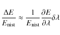
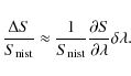
Our structure was optimized by using a singular value decomposition
(Golub & Van Loan 1989) method to give best agreement with
selected NIST (2008) values for the level energies and line
strengths. The orbitals were determined by using a
Thomas-Fermi-Dirac-Amaldi (TFDA) statistical potential. To optimize
our structure we make use of scale factors for the wavefunctions in
each orbital. These scale factors, or ![]() s, enable us to adjust
the radial extent of the wavefunctions for each orbital. These small
adjustments allow some fine tuning of the atomic structure and the
associated line strengths.
s, enable us to adjust
the radial extent of the wavefunctions for each orbital. These small
adjustments allow some fine tuning of the atomic structure and the
associated line strengths.
We developed a code (LAMDA) to optimize our atomic structure by
varying the ![]() scale factors. This is similar to the
approach of Bautista (2008). In order to monitor and
compare the quality of our atomic structure, we make use of the NIST
table quantities. The selected quantities that we wish to reproduce
are the NIST energy (levels or terms)
scale factors. This is similar to the
approach of Bautista (2008). In order to monitor and
compare the quality of our atomic structure, we make use of the NIST
table quantities. The selected quantities that we wish to reproduce
are the NIST energy (levels or terms)
![]() ,
and either the
line strengths
,
and either the
line strengths
![]() ,
the collision strengths
,
the collision strengths
![]() ,
or Einstein coefficients
,
or Einstein coefficients
![]() .
In our modeling we prefer to
use line strengths due to their greater independence of energies.
Some of the NIST line strengths
.
In our modeling we prefer to
use line strengths due to their greater independence of energies.
Some of the NIST line strengths
![]() have a big uncertainty
listed on the tables, therefore our code is able to chose the ones
that have a small listed error, in this case we chose line strengths
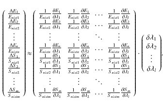
with less than 10% error. We optimized on the 114 NIST energy levels
that were also in our structure calculation. Since the energies and
line strengths depend upon the scale factors (
have a big uncertainty
listed on the tables, therefore our code is able to chose the ones
that have a small listed error, in this case we chose line strengths
with less than 10% error. We optimized on the 114 NIST energy levels
that were also in our structure calculation. Since the energies and
line strengths depend upon the scale factors (![]() s), we
linearize both and approximate the relation between our chosen NIST
quantities and our modeled values as
s), we
linearize both and approximate the relation between our chosen NIST
quantities and our modeled values as
![]() ,
and
,
and
![]() .
.
To include both of these different quantities in our optimization we
normalize both of them with their respective NIST values, therefore
 |
(1) |
 |
(2) |
This way we get our complete model for any n number of energies, any m number of line strengths, and l number of scale factors as
 |
(3) |
We rewrite the model in vector notation as
| (4) |
Where
- the columns of
 form a set of orthonormal
input or analyzing basis vector directions for
form a set of orthonormal
input or analyzing basis vector directions for
 ;
;
- the columns of
 form a set orthonormal output
basis vector directions for ;
form a set orthonormal output
basis vector directions for ;
- the matrix
 contains the singular values, which can
be thought of as scalar gain controls by which each
corresponding input is multiplied to give a corresponding
output.
contains the singular values, which can
be thought of as scalar gain controls by which each
corresponding input is multiplied to give a corresponding
output.
| (5) |
The matrix
With this restriction in place we select the p number of singular values to compute the singular values inverse matrix
We obtained good results from the optimization process with a
![]() before the optimization and a
before the optimization and a
![]() after
the optimization. That represents an improvement of 92.01% in our
after
the optimization. That represents an improvement of 92.01% in our
![]() value. We found that this optimization method gave us better
results than AUTOSTRUCTURE's default optimization of minimization of
energies which gives a
value. We found that this optimization method gave us better
results than AUTOSTRUCTURE's default optimization of minimization of
energies which gives a
![]() .
We also found better average
percentage difference within the first 9 energy levels and those from
NIST. AUTOSTRUCTURE's default optimization gives a 20.03% difference
while our optimization method gives 4.83%.
.
We also found better average
percentage difference within the first 9 energy levels and those from
NIST. AUTOSTRUCTURE's default optimization gives a 20.03% difference
while our optimization method gives 4.83%.
2.2 The R-Matrix method
The scattering calculation was performed with our set of parallel
R-Matrix programs (Mitnik et al. 2003; Ballance &
Griffin 2004), which are extensively modified versions of
the serial RMATRIX I programs of Berrington et al.
(1995). The method is based on partitioning the
configuration space in to two regions by a sphere of radius a
centered on the target nucleus. In the internal region ![]() electron exchange and correlation between the scattered electron and
the the N-electron target atom or ion are important and the
(N+1)-electron collision complex behaves in a similar way to a bound
state. In the external region r > a electron exchange between the
scattered electron and the target can be neglected if the radius a
is chosen so that the charge distribution of the target is contained
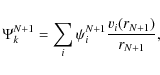
within the sphere. Outside the R-Matrix box, the total wavefunction
for a given LS symmetry is expanded in basis states given by:
electron exchange and correlation between the scattered electron and
the the N-electron target atom or ion are important and the
(N+1)-electron collision complex behaves in a similar way to a bound
state. In the external region r > a electron exchange between the
scattered electron and the target can be neglected if the radius a
is chosen so that the charge distribution of the target is contained
within the sphere. Outside the R-Matrix box, the total wavefunction
for a given LS symmetry is expanded in basis states given by:
 |
(7) |
where vi(r) are radial continuum functions obtained by solution of radial asymptotic coupled differential equations. The inner and outer solutions are matched at the edge of the R-Matrix box to extract collision strengths.
In this paper we have employed both the Breit-Pauli and ICFT
(Intermediate Coupling Frame Transformation) R-Matrix methods for
electron-impact excitation (Griffin et al. 1998). The
original impetus for the ICFT approach was to reduce the time
consuming diagonalisation of each large Breit-Pauli Hamiltonian. In
the ICFT method, as each partial wave includes only the mass-velocity
and Darwin corrections to the LS![]() N+1 Hamiltonian and omits the
spin-orbit interaction; this greatly reduces the size of each
symmetric matrix to be diagonalised. In the outer region, the
resulting LS-coupled scattering S- or K-matrices are transformed to jK
coupling by means of an algebraic transformation to provide
level-to-level excitation cross sections. This transformation involves
TCC's (Term Coupling Coefficients) which are calculated from a
Breit-Pauli structure calculation (including spin-orbit interaction),
to express the eigenvectors for the resulting levels as linear
combinations of the multi-configuration mixed terms. The coefficients
of this expansion are the TCCs. With the implementation of a parallel
versions of our codes, and for the scale of calculations described in
this paper, both methods would take a similar amount of time, however
the ICFT approach remains better suited for small memory serial
machines and/or small parallel clusters as calculations increase in
size. The consistency of results between ICFT and Breit-Pauli
calculations reported later in this paper should provide a lower bound
on the error we would expect in the subsequent collisional-radiative
modeling. Effective collision strengths are generated from our
R-Matrix collision strength data via convolution with a Maxwellian
electron distribution.
N+1 Hamiltonian and omits the
spin-orbit interaction; this greatly reduces the size of each
symmetric matrix to be diagonalised. In the outer region, the
resulting LS-coupled scattering S- or K-matrices are transformed to jK
coupling by means of an algebraic transformation to provide
level-to-level excitation cross sections. This transformation involves
TCC's (Term Coupling Coefficients) which are calculated from a
Breit-Pauli structure calculation (including spin-orbit interaction),
to express the eigenvectors for the resulting levels as linear
combinations of the multi-configuration mixed terms. The coefficients
of this expansion are the TCCs. With the implementation of a parallel
versions of our codes, and for the scale of calculations described in
this paper, both methods would take a similar amount of time, however
the ICFT approach remains better suited for small memory serial
machines and/or small parallel clusters as calculations increase in
size. The consistency of results between ICFT and Breit-Pauli
calculations reported later in this paper should provide a lower bound
on the error we would expect in the subsequent collisional-radiative
modeling. Effective collision strengths are generated from our
R-Matrix collision strength data via convolution with a Maxwellian
electron distribution.
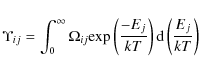 |
(8) |
where Ej is the energy of the outgoing electron and
 |
(9) | ||
| (10) |
where Eij is the energy of the transition i to j, and C is an arbitrary constant. We will use a C-value of 5.0 to compare with the Burgess-Tully results shown in Galavis et al. (1998).
2.3 Collisional radiative model
We use the ADAS (http://www.adas.ac.uk)
suite of codes for our population and
emission modeling. These codes are based on collisional-radiative
theory, first developed by Bates et al. (1962) and later
generalized by Summers & Hooper (1983). The method
aims to encompass both the low density coronal and high density local
thermodynamic equilibrium description of an ion and to track the
shifting balance between radiative and collisional processes. The ion
consists of a set of levels with radiative and collisional couplings.
Ionization and recombination to and from metastables of the next
ionization stage (i.e. the plus ion stage) are included. The time
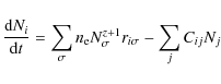
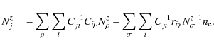
dependence of the population (Ni) of an arbitrary level i in ion
stage +z is given by
| |
= | ||
 |
|||
 |
|||
| (11) |
where
 |
(12) |
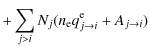
with a populating term for
 |
(13) |
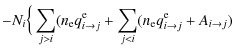
a loss term
 |
(14) |
and a composite recombination coefficient
 |
(15) |
A spectral line intensity ratio for a homogeneous plasma is evaluated via
 |
(16) |
and an energy intensity ratio is given by
| |
= |  |
|
| = |  |
(17) |
When comparing with spectral line ratios observed from planetary nebulae we will use this latter equation, since the observations will be of the energy absorbed at a given wavelength.
3 Results
Our results can be split into three main areas: structure, collisional data and emission modeling.
3.1 Structure
Our final optimized structure consisted of configurations
3s23p4, 3s3p5, 3p6, 3p53d, and 3s23p3nl (3d ![]() nl
nl ![]() 5s), giving a total of 186 levels. Our optimized lambda
parameters, obtained using our singular value decomposition code, are
given in Table 1. Our structure was optimized using
NIST energy levels and line strengths. The level energies from our
structure calculation are given in Table 2. We show
results for the first 29 levels, the remaining energies can be found
in the archived datafile (see http://www-cfadc.phy.ornl.gov/data_and_codes).
The average percentage
error between our calculated energies and the NIST energies is 3.46%.
The largest error is for the 3s23p4(1D2) level. Because of
the diagnostic importance of the transitions within the 3p4
configuration, we will shift to NIST values all the energies
associated with the 3p4 and 3s3p5 configurations. This will be
described in the next section.
5s), giving a total of 186 levels. Our optimized lambda
parameters, obtained using our singular value decomposition code, are
given in Table 1. Our structure was optimized using
NIST energy levels and line strengths. The level energies from our
structure calculation are given in Table 2. We show
results for the first 29 levels, the remaining energies can be found
in the archived datafile (see http://www-cfadc.phy.ornl.gov/data_and_codes).
The average percentage
error between our calculated energies and the NIST energies is 3.46%.
The largest error is for the 3s23p4(1D2) level. Because of
the diagnostic importance of the transitions within the 3p4
configuration, we will shift to NIST values all the energies
associated with the 3p4 and 3s3p5 configurations. This will be
described in the next section.
Table 1:
Final ![]() values for the 1s-5s orbitals.
values for the 1s-5s orbitals.
Table 2: Energies in Rydbergs for the lowest 29 levels of Ar2+.
As a further check on our structure, we present a selection of our
calculated radiative rates in Table 3, we show our
calculated radiative rates compared with NIST (2008) values and
the calculations of Mendoza & Zeippen (1983). The
average percentage difference between the NIST Einstein A coefficients
and ours is 65.36%. We note that for most of the transitions the NIST
uncertainty estimates on the Einstein A coefficients are 25% or
![]() 50%, our Einstein A coefficients are in general within the
NIST uncertainty estimates. In the dataset we use for our emission
modeling the Einstein A coefficients for transitions within the
3s23p4 configuration will be replaced by the calculated values
of Mendoza & Zeippen (1983). This will allow us to make
a direct comparison with previous modeling results from the
literature, highlighting the differences due to the excitation data
only. However, our final archived dataset will contain our calculated
Einstein A coefficients.
50%, our Einstein A coefficients are in general within the
NIST uncertainty estimates. In the dataset we use for our emission
modeling the Einstein A coefficients for transitions within the
3s23p4 configuration will be replaced by the calculated values
of Mendoza & Zeippen (1983). This will allow us to make
a direct comparison with previous modeling results from the
literature, highlighting the differences due to the excitation data
only. However, our final archived dataset will contain our calculated
Einstein A coefficients.
3.2 Scattering calculations
The orbitals used in our R-Matrix calculations were generated from
the AUTOSTRUCTURE (Badnell 1986) code using the optimized
![]() parameters from Table 1. Our exchange
calculation included partial waves from L=0 to L=14 (J=0.5 to
J=11.5 for the Breit-Pauli calculation). The non-exchange
calculation went from L=10 up to L=40 (J=12.5 to J=37.5). The
contributions from higher partial waves were then calculated for
dipole transitions using the method originally described by Burgess
(1970) and for the non-dipole transitions assuming a
geometric series in L, using energy ratios, with special procedures
for handling transitions between nearly degenerate terms. Using
AUTOSTRUCTURE (Badnell 1986), we also calculated infinite
energy Bethe/Born limits, allowing us to extend the effective
collision strengths and rate coefficients to temperature ranges above
the highest calculated collision strength. In our outer region
calculations, we used 80 000 energy mesh points over the resonance
region (up to 6 Ryd) and 500 energy mesh points for the higher
energies (6 Ryd to 12 Ryd).
parameters from Table 1. Our exchange
calculation included partial waves from L=0 to L=14 (J=0.5 to
J=11.5 for the Breit-Pauli calculation). The non-exchange
calculation went from L=10 up to L=40 (J=12.5 to J=37.5). The
contributions from higher partial waves were then calculated for
dipole transitions using the method originally described by Burgess
(1970) and for the non-dipole transitions assuming a
geometric series in L, using energy ratios, with special procedures
for handling transitions between nearly degenerate terms. Using
AUTOSTRUCTURE (Badnell 1986), we also calculated infinite
energy Bethe/Born limits, allowing us to extend the effective
collision strengths and rate coefficients to temperature ranges above
the highest calculated collision strength. In our outer region
calculations, we used 80 000 energy mesh points over the resonance
region (up to 6 Ryd) and 500 energy mesh points for the higher
energies (6 Ryd to 12 Ryd).
Table 3: Comparisons of selected radiative rates for transitions in Ar2+.
It has been shown by Griffin et al. (1998) that an
ICFT calculation would produce the same results as a Breit-Pauli
calculation. As a check on our calculation we performed an ICFT and a
Breit-Pauli calculation using the same set of radial orbitals for
both. Figure 1 shows the ICFT and Breit-Pauli
collision strength for the 3s23p4(1P2)
![]() 3s23p4(1D2) transition. Although small differences can be
seen, the two calculations are clearly very close to each other.
3s23p4(1D2) transition. Although small differences can be
seen, the two calculations are clearly very close to each other.
This level of agreement was typical for the collision strengths calculated. The 186 levels in our Ar2+ calculation give rise to 17 205 transitions. We used the scatterplot method of Witthoeft et al. (2007) to compare the Maxwellian effective collision strengths for all of the transitions at one time. This method takes the ratio of effective collision strengths for all transitions for a given temperature and plots this ratio against one of the effective collision strengths. Thus a ratio of one would indicate the datasets are the same. This method also allows one to see the strength of the transitions that are in disagreement. We chose an electron temperature of 1.55 eV as one typical of planetary nebula and low enough to strongly sample the resonance region of the collision strengths. Of the 17 205 transitions, 82% of the ICFT effective collision strengths are within 10% of the Breit-Pauli values. 94% of the ICFT effective collision strengths are within 20% of the Breit-Pauli values and 98% are within 40%. Of the transitions that show a difference, they are in general for weaker transitions involving highly excited levels with effective collision strengths that are extremely sensitive to the resonance contributions on top of a weak background. These transitions are not likely to make a difference in population modeling. For example, the transitions within the 3p4 configuration are within 4% of each other. Population modeling using the ICFT and Breit-Pauli datasets produces essentially the same excited populations for all cases we investigated. For the final data set we used the Breit-Pauli results.
![\begin{figure}
\par\includegraphics[width=9cm,clip]{1743fig1.eps}
\end{figure}](/articles/aa/full_html/2009/24/aa11743-09/img120.png) |
Figure 1:
Comparison of the ICFT and Breit-Pauli collision strengths
for the 3s23p4(3P2)
|
| Open with DEXTER | |
![\begin{figure}
\par\includegraphics[width=8.4cm,clip]{1743fig2.eps}
\end{figure}](/articles/aa/full_html/2009/24/aa11743-09/img121.png) |
Figure 2: Scatter plot showing the ratio of effective collision strengths at Te = 1.55 eV between two Breit-Pauli R-Matrix calculations. One had 40 000 energy mesh point in the resonance region, the other had 80 000 energy mesh points in the resonance region. We show the ratio of effective collision strength vs. the effective collision strength of the 40 000 energy mesh calculation. |
| Open with DEXTER | |
To provide the most accurate data for modeling, a Breit-Pauli calculation was then done with shifts to NIST energies for the first 9 energy levels, due to their importance in spectral line diagnostics. To test the convergence of our energy mesh over the resonance region we performed a series of calculations using different meshes, namely 10 000, 20 000, 40 000 and 80 000 mesh points in the resonance region. We calculated Maxwellian averaged effective collision strengths for each of these meshes and compared the files. Figure 2 shows a scatterplot comparison of our Breit-Pauli calculation using 40 000 and 80 000 mesh points in the resonance region. Of the 17 205 transitions, most are converged, with a few outliers. There was a progression of convergence as the mesh was increased. For example, comparing calculations with 20 000 and 40 000 energy mesh points in the resonance region we found that 93.4% of the transitions were converged to within 2% of each other. Comparing the 20 000 and 40 000 energy mesh point calculations, 96.4% of the transitions were converged to within 2% of each other. Finally, comparing the 40 000 and 80 000 energy mesh point calculations, 98.4% of the transitions were converged to within 2% of each other, with 95.5% being within 1%. Thus, we believe that our 80 000 enegy mesh point calculation is converged.
![\begin{figure}
\par\includegraphics[width=8.3cm,clip]{1743fig3.eps}
\end{figure}](/articles/aa/full_html/2009/24/aa11743-09/img122.png) |
Figure 3:
Comparison of selected Breit-Pauli collision strengths (with
energy shifts included for the first 9 energy levels) with
Johnson & Kingston (1990).
Plot a) shows the 3p4(3P2)
|
| Open with DEXTER | |
Of the previous R-Matrix calculations, we can compare with the collision strengths from Johnson & Kingston (1990), see Fig. 3 for a comparison of a selection of transitions. There are clear differences in the resonance positions and heights, with the background collision strengths being in good agreement. The differences in the resonance contributions may be due to the well known problems with the JAJOM method (Griffin et al. 1998) that was used by Johnson & Kingston (1990) to transform the LS results to LSJ resolution.
We can compare our effective collision strength results with the IRON
project data of (Galavis et al. 1995), and with the
tabulated values of Johnson & Kingston (1990).
Figure 4 shows the comparison for a
selection of transitions. Table 4 shows our
calculated effective collision strengths for transitions between the
3s23p4 levels. At the highest temperatures, our effective
collision strengths are consistently higher than the previous
calculations. Since we have a similar background cross-section, the
differences are due to the extra resonance channels included in
our calculation, and to a lesser extent differences in our top-up
procedures. Most transitions show differences at low temperatures
where sensitivity to the low energy resonance contribution is
strongest. This is particularly true for the transitions
3p4(3P2)
![]() 3p4(1S0) and
3p4(1D2)
3p4(1S0) and
3p4(1D2)
![]() 3p4(1S0), shown in
Fig. 4e and f). In both cases our
effective collision strengths are smaller than previous calculations
at the lowest temperatures. This is most likely due to the
contributions from near threshold resonances. For example, the
3p4(1D2)
3p4(1S0), shown in
Fig. 4e and f). In both cases our
effective collision strengths are smaller than previous calculations
at the lowest temperatures. This is most likely due to the
contributions from near threshold resonances. For example, the
3p4(1D2)
![]() 3p4(1S0) transition has
contribution due to a reported 3s3p5(3P)3d(2P) resonance that
occurs at the excitation threshold in the previous R-Matrix
calculations of Johnson & Kingston (1990). Galavis et al. (1995) also point out the large contribution from a
near threshold resonance in their calculation of this transition. The
near threshold resonance in the 3p4(3P)
3p4(1S0) transition has
contribution due to a reported 3s3p5(3P)3d(2P) resonance that
occurs at the excitation threshold in the previous R-Matrix
calculations of Johnson & Kingston (1990). Galavis et al. (1995) also point out the large contribution from a
near threshold resonance in their calculation of this transition. The
near threshold resonance in the 3p4(3P)
![]() 3p4(1S) transition is likely to be due to the same resonance. We
do not see this near threshold resonance in our calculations for
either of these transitions. As will be seen later, these two
transitions are key for spectral diagnostics. Thus, we performed a
smaller R-Matrix calculation, using the same configurations as
Johnson & Kingston (1990). In this calculation we do see
a near threshold resonance in the 3p4(1D2)
3p4(1S) transition is likely to be due to the same resonance. We
do not see this near threshold resonance in our calculations for
either of these transitions. As will be seen later, these two
transitions are key for spectral diagnostics. Thus, we performed a
smaller R-Matrix calculation, using the same configurations as
Johnson & Kingston (1990). In this calculation we do see
a near threshold resonance in the 3p4(1D2)
![]() 3p4(1S0) transition, as seen in previous work. We identified
the resonances as belonging to the J=3/2 partial wave. Investigation
of the eigenphase sum shows that this broad resonance belongs to the
3s3p53d configuration, and is shifted to lower energy in our larger
Breit-Pauli calculation. Thus it does not contribute to our collision
strength. Our resonance position should be more accurate, due to the
larger number of configurations in our structure calculation. However,
this resonance is very close to the excitation threshold and is
clearly sensitive to configuration interaction effects. Experimental
measurements of this collision strength would be very useful.
3p4(1S0) transition, as seen in previous work. We identified
the resonances as belonging to the J=3/2 partial wave. Investigation
of the eigenphase sum shows that this broad resonance belongs to the
3s3p53d configuration, and is shifted to lower energy in our larger
Breit-Pauli calculation. Thus it does not contribute to our collision
strength. Our resonance position should be more accurate, due to the
larger number of configurations in our structure calculation. However,
this resonance is very close to the excitation threshold and is
clearly sensitive to configuration interaction effects. Experimental
measurements of this collision strength would be very useful.
![\begin{figure}
\par\includegraphics[width=9cm,clip]{1743fig4.eps}
\end{figure}](/articles/aa/full_html/2009/24/aa11743-09/img123.png) |
Figure 4:
Comparison of selected Breit-Pauli effective collision
strengths (with energy shifts included for the first 9
energy levels) with Johnson & Kingston (1990)
and with Galavis et al. (1995,1998).
Plot a) shows the 3p4(3P2)
|
| Open with DEXTER | |
Table 4: Effective collision strengths for transitions between the 3s23p4 levels.
At higher temperatures for the 3p4(1D2)
![]() 3p4(1S0) transition we verify the findings of Burgess et al.
(1997), and Galavis et al. (1998) that
contributions from higher partial waves are required for the effective
collision strength to tend to the right limit point. We plot our
results for this transition in a Burgess-Tully plot in
Fig. 5 to highlight the high energy
behaviour. Our results go to a limit point of 1.72, close to the value
of 1.68 expected by Burgess et al. (1997). As pointed out
by Galavis et al. (1998), the rise in slope of the
Burgess-Tully plot towards the limit point does not happen until
relatively close to the limit point.
3p4(1S0) transition we verify the findings of Burgess et al.
(1997), and Galavis et al. (1998) that
contributions from higher partial waves are required for the effective
collision strength to tend to the right limit point. We plot our
results for this transition in a Burgess-Tully plot in
Fig. 5 to highlight the high energy
behaviour. Our results go to a limit point of 1.72, close to the value
of 1.68 expected by Burgess et al. (1997). As pointed out
by Galavis et al. (1998), the rise in slope of the
Burgess-Tully plot towards the limit point does not happen until
relatively close to the limit point.
![\begin{figure}
\par\includegraphics[angle=-90,width=9cm,clip]{1743fig5.eps}
\end{figure}](/articles/aa/full_html/2009/24/aa11743-09/img124.png) |
Figure 5:
Burgess Tully plot of effective collision strength vs.
reduced temperature (X). Results are shown for transition
3p4(1D2)
|
| Open with DEXTER | |
3.3 Emission modeling
Our Breit-Pauli atomic dataset was used to model commonly observed
forbidden transitions of Ar III. Our modeling data consists of the
Breit-Pauli excitation data, including shifts to NIST energies for the
first 9 levels. Our dipole Einstein A coefficients were evaluated in
our R-Matrix calculation. Our non-dipole Einstein A coefficients
came from an AUTOSTRUCTURE calculation. For the purpose of the
modeling work in this paper we use the same Einstein A coefficients
for transitions within the 3p4 configuration as those of Mendoza
& Zeippen (1983). These were the Einstein A coefficients
used in previous emission models using R-Matrix data from Keenan &
McCann (1990), and Keenan & Conlon (1993).
Using the same Einstein A coefficients will allow us to highlight
differences in emission modeling due to the excitation collision
data. The final set of data that is available online will include our
computed Einstein A coefficients for all the transitions. We first
consider the temperature sensitive energy intensity ratio
| R1 | = | ||
| = |  |
(18) |
where the numbers in the subscripts of N and A denote the index numbers of the energy levels involved in the transitions. The ratio is insensitive to electron density up to
![\begin{figure}
\par\includegraphics[width=9cm,clip]{1743fig6.eps}
\end{figure}](/articles/aa/full_html/2009/24/aa11743-09/img128.png) |
Figure 6:
R1 line ratio as a function of electron temperature. The
results are calculated at
|
| Open with DEXTER | |
Our results for the density sensitive energy intensity ratio
| R2 | = | ||
| = |  |
(19) |
is shown in Fig. 7. We again compare with calculations using the data of Johnson & Kingston (1990) and the data of Galavis et al. (1995). The modeling using the Johnson and Kingston data is equivalent to the ratio shown in Keenan & Conlon (1993). For each temperature one can see that all the R2 ratios go from their coronal value at low densities to their local thermodynamic equilibrium value by
![\begin{figure}
\par\includegraphics[width=9cm,clip]{1743fig7.eps}
\end{figure}](/articles/aa/full_html/2009/24/aa11743-09/img135.png) |
Figure 7: R2 line ratio as a function of electron density. The results are calculated for a range of electron temperatures, namely 5000, 8000, 10 000, 15 000, 20 000 and 30 000 K. The lowest line ratio is the 5000 K results, with the higher ratios showing the progressively higher temperature results. The solid line shows the results using the new R-Matrix Breit-Pauli collision data. The dot-dashed line show the results using the data of Johnson & Kingston (1990) and the dashed line shows the results using the data of Galavis et al. (1995). |
| Open with DEXTER | |
4 Conclusions
The results of a 186 level R-Matrix calculations are presented for Ar2+.
- 1.
- The results from an ICFT calculation are shown to be close to those from a Breit-Pauli calculation. Our final R-Matrix calculation consists of a Breit-Pauli calculation with the first 9 levels shifted to NIST energies.
- 2.
- We compare the results of this calculation with literature values for transitions within the 3p4 configuration, finding differences at low temperatures due to low energy resonance contributions.
- 3.
- We calculate one temperature sensitive and one density sensitive line ratio, finding that our new data does not make a significant differences to the temperature diagnostic, but does have a sizeable affect on the density diagnostic, compared to values calculated using previous R-Matrix data.
- 4.
- Our final effective collision strengths are now available on the Oak Ridge National Laboratory Atomic Data Web (http://www-cfadc.phy.ornl.gov/data_and_codes) and in the ADAS (http://www.adas.ac.uk) database. The data presented at Tables 2, 3, and 4 is also available in electronic form at the CDS.
Acknowledgements
This work was supported by US DoE grant DE-FG02-99ER54367 to Rollins College and US DoE grants DE-FG05-96-ER54348 and DE-FG02-01ER54633 to Auburn University. Most of the computational work was carried out at the National Energy Research Scientific Computing Center in Oakland, California, and at the Alabama Supercomputer in Huntsville, Alabama.
References
- Aller, L. H., & Keyes, C. D. 1987, ApJS, 65, 405 [NASA ADS] [CrossRef] (In the text)
- Badnell, N. R. 1986, J. Phys. B, 19, 3827 [NASA ADS] [CrossRef] (In the text)
- Badnell, N. R., Pindzola, M. S., Bray, I., & Griffin, D. C. 1998, J. Phys. B, 31, 911 [NASA ADS] [CrossRef]
- Ballance, C. P., & Griffin, D. C. 2004, J. Phys. B, 37, 2943 [NASA ADS] [CrossRef] (In the text)
- Ballance, C. P., & Griffin, D. C. 2008, J. Phys. B. 41, 065201 (In the text)
- Ballance, C. P., & Griffin, D. C. 2008, J. Phys. B, 41, 195205 [NASA ADS] [CrossRef] (In the text)
- Bates, D. R., Kingston, A. E., & McWhirter, R. W. P. 1962, Proc. Royal Soc. London, 267, 297 [NASA ADS] (In the text)
- Bautista, M. A. 2008, J. Phys. B: At. Mol. Opt. Phys, 41, 65701 [CrossRef] (In the text)
- Berrington, K. A., Eissner, W. B., & Norrington, P. H. 1995, Comput. Phys. Commun., 92, 290 [NASA ADS] [CrossRef] (In the text)
- Boffard, J. B., Chiaro, B., Lin, C. C., & Weber, T. 2007, Atomic Data and Nuclear Data Tables, 93, 831 [NASA ADS] [CrossRef] (In the text)
- Burgess, A. 1970, J. Phys. B, 7, L364 [CrossRef] (In the text)
- Burgess, A., Chidichimo, M. C., & Tully, J. A. 1997, J. Phys. B, 30, 33 [NASA ADS] [CrossRef] (In the text)
- De Robertis, M. M., Dufour, R. J., & Hunt, R. W. 1987, J. Roy. Astron. Soc. Can., 81, 195 [NASA ADS] (In the text)
- Galavis, M. E., Mendoza, C., & Zeippen, C. J. 1995, A&AS, 111, 347 [NASA ADS] (In the text)
- Galavis, M. E., Mendoza, C., & Zeippen, C. J. 1998, A&AS, 133, 245 [NASA ADS] [CrossRef] [EDP Sciences] (In the text)
- Golub, G. H., & Van Loan, C.F. 1989, Matrix Computations, 2nd edn. (Baltimore: Johns Hopkins University Press), 8.3, Chap. 12 (In the text)
- Griffin, D. C., Badnell, N. R., & Pindzola, M. S. 1998, J. Phys. B, 31, 3713 [NASA ADS] [CrossRef] (In the text)
- Griffin, D. C., Ballance, C. P., Loch, S. D., & Pindzola, M. S. 2007, J. Phys. B, 40, 4537 [NASA ADS] [CrossRef] (In the text)
- Johnson, C. T., & Kingston, A.E. 1990, J. Phys. B, 23, 3393 [NASA ADS] [CrossRef] (In the text)
- Jung, R. O., Boffard, J. B., Anderson, L. W., & Lin, C. C. 2007, Phys. Rev. Lett., 75, 052707 [NASA ADS] (In the text)
- Keenan, F. P., & McCann, S. M. 1990, J. Phys. B, 23, L423 [NASA ADS] [CrossRef] (In the text)
- Keenan, F. P., & Conlon, E. S. 1993, ApJ, 410, 426 [NASA ADS] [CrossRef] (In the text)
- Madison, D. H., Dasgupta, A., Bartschat, K., & Vaid, D. 2004, J. Phys. B, 37, 1073 [NASA ADS] [CrossRef] (In the text)
- Mendoza, C., & Zeippen, C. J. 1983, MNRAS, 202, 981 [NASA ADS] (In the text)
- Mitnik, D. M., Griffin, D. C., Ballance, C. P., & Badnell, N. R. 2003, J. Phys. B, 36, 717 [NASA ADS] [CrossRef] (In the text)
- Perez-Montero, E., Hagele, G. F., Contini, T., & Diaz, A. I. 2007, MNRAS, 381, 125 [NASA ADS] [CrossRef] (In the text)
- Pipher, J. L., Helfer, H. L., Herter, T., et al. 1984, ApJ, 285, 174 [NASA ADS] [CrossRef] (In the text)
- Ralchenko, Yu., Kramida, A. E., Reader, J., & NIST ASD Team. 2008, NIST Atomic Spectra Database, version 3.1.5, http://physics.nist.gov/asd3, National Institute of Standards and Technology, Gaithersburg, MD (In the text)
- Saraph, H. E. 1978, Comput. Phys. Commun., 15, 247 [NASA ADS] [CrossRef] (In the text)
- Strinic, A. I., Malovic, G. N., Petrovic, Z. L., & Sadeghi, N. 2007, Plasma, 75, 052707 (In the text)
- Summer, H. P., & Hooper, M. 1983, Plasma Physics, 25, 1311 [NASA ADS] [CrossRef] (In the text)
- Whyte, D. G., Jernigan, T. C., Humphreys, D. A., et al. 2002, Phys. Rev. Lett., 89, 055001 [NASA ADS] [CrossRef] (In the text)
- Witthoeft, M. C., Whiteford, A. D., & Badnell, N. R. 2007, J. Phys. B, 40, 2969 [NASA ADS] [CrossRef] (In the text)
Footnotes
- ... online
![[*]](/icons/foot_motif.png)
- Tables 2-4 are also available in electronic form at the CDS viaanonymous ftp to cdsarc.u-strasbg.fr (130.79.128.5) or via http://cdsweb.u-strasbg.fr/cgi-bin/qcat?J/A+A/500/1253
All Tables
Table 1:
Final ![]() values for the 1s-5s orbitals.
values for the 1s-5s orbitals.
Table 2: Energies in Rydbergs for the lowest 29 levels of Ar2+.
Table 3: Comparisons of selected radiative rates for transitions in Ar2+.
Table 4: Effective collision strengths for transitions between the 3s23p4 levels.
All Figures
| |
Figure 1:
Comparison of the ICFT and Breit-Pauli collision strengths
for the 3s23p4(3P2)
|
| Open with DEXTER | |
| In the text | |
| |
Figure 2: Scatter plot showing the ratio of effective collision strengths at Te = 1.55 eV between two Breit-Pauli R-Matrix calculations. One had 40 000 energy mesh point in the resonance region, the other had 80 000 energy mesh points in the resonance region. We show the ratio of effective collision strength vs. the effective collision strength of the 40 000 energy mesh calculation. |
| Open with DEXTER | |
| In the text | |
| |
Figure 3:
Comparison of selected Breit-Pauli collision strengths (with
energy shifts included for the first 9 energy levels) with
Johnson & Kingston (1990).
Plot a) shows the 3p4(3P2)
|
| Open with DEXTER | |
| In the text | |
| |
Figure 4:
Comparison of selected Breit-Pauli effective collision
strengths (with energy shifts included for the first 9
energy levels) with Johnson & Kingston (1990)
and with Galavis et al. (1995,1998).
Plot a) shows the 3p4(3P2)
|
| Open with DEXTER | |
| In the text | |
| |
Figure 5:
Burgess Tully plot of effective collision strength vs.
reduced temperature (X). Results are shown for transition
3p4(1D2)
|
| Open with DEXTER | |
| In the text | |
| |
Figure 6:
R1 line ratio as a function of electron temperature. The
results are calculated at
|
| Open with DEXTER | |
| In the text | |
| |
Figure 7: R2 line ratio as a function of electron density. The results are calculated for a range of electron temperatures, namely 5000, 8000, 10 000, 15 000, 20 000 and 30 000 K. The lowest line ratio is the 5000 K results, with the higher ratios showing the progressively higher temperature results. The solid line shows the results using the new R-Matrix Breit-Pauli collision data. The dot-dashed line show the results using the data of Johnson & Kingston (1990) and the dashed line shows the results using the data of Galavis et al. (1995). |
| Open with DEXTER | |
| In the text | |
Copyright ESO 2009
Current usage metrics show cumulative count of Article Views (full-text article views including HTML views, PDF and ePub downloads, according to the available data) and Abstracts Views on Vision4Press platform.
Data correspond to usage on the plateform after 2015. The current usage metrics is available 48-96 hours after online publication and is updated daily on week days.
Initial download of the metrics may take a while.