| Issue |
A&A
Volume 499, Number 1, May III 2009
|
|
|---|---|---|
| Page(s) | 17 - 20 | |
| Section | Astrophysical processes | |
| DOI | https://doi.org/10.1051/0004-6361/200911701 | |
| Published online | 25 March 2009 | |
Linear force-free field of a toroidal symmetry
(Research Note)
E. Romashets1,2,3 - M. Vandas4
1 - Center for Plasma Astrophysics, K.U. Leuven 3001, Belgium
2 - Solar Observatory, Prairie View A& M University,
Prairie View 77446, USA
3 - Institute of Terrestrial Magnetism, Ionosphere,
and Radio Wave Propagation of Russian Academy of Sciences,
Troitsk 142190, Russia
4 - Astronomical Institute, Academy of Sciences of the Czech
Republic, Bocní II 1401, 141 31 Praha 4, Czech Republic
Received 22 January 2009 / Accepted 1 March 2009
Abstract
Context. Interplanetary flux ropes are often described by linear force-free fields. To account for their curvature, toroidal configurations valid for large aspect ratios are used. However, in some cases, flux ropes need to be approximated by a toroid with a low aspect ratio.
Aims. The aim is to find an analytical description of a linear force-free magnetic field of toroidal geometry, not restricted to large aspect ratios.
Methods. The solution is found as a superposition of fields given by linear force-free cylinders tangential to a generating toroid.
Results. The obtained solution describes toroidal flux ropes with reasonable shapes and magnetic field values. The field is exactly linear force-free for arbitrary aspect ratios. The new solution can be applied for solar and interplanetary flux ropes, astrophysical objects, and laboratory plasma.
Key words: magnetic fields - solar wind - Sun: coronal mass ejections (CMEs)
1 Introduction
Interplanetary magnetic flux ropes are commonly observed in the solar wind. The term magnetic cloud was proposed by Klein & Burlaga (1982) for such larger objects with distinct properties of higher magnetic field, smooth rotation of the magnetic field vector, and low proton temperature of the solar wind plasma. They have a loop-like shape, so they could be described by a toroidal flux rope.The field of application of toroidal force-free fields is not only interplanetary magnetic structures or solar flux ropes, but also laboratory plasma and various astrophysical objects. For example, symbiotic stars R Aqr contain a white dwarf with an X-ray jet. The flow in the jet is curved (Ragland et al. 2008) and is governed by a strong magnetic field of the main star which is of the order of 105 T (Hollis & Koupelis 2000). Taking into account that temperature of the flow plasma is about 106 K and the density is of the order of 103 cm-3, one can infer that there is a force-free plasma in the flow.
Interplanetary magnetic clouds are usually modelled locally as straight cylinders with a linear force-free field (e.g., Burlaga 1988; Lepping et al. 1990, 2006). Globally, however, magnetic clouds as interplanetary flux ropes have a loop-like shape (Lepping et al. 1990), i.e., they are curved. In such cases, where curvature could play a role, approximation of interplanetary flux ropes by a part of a toroid would be more appropriate. Marubashi (1997) was first to discuss the implications of this global shape for the interpretation of magnetic cloud observations and approximated clouds by a toroidal flux rope. Before that, a first attempt to fit magnetic clouds with a toroidal configuration was made by Ivanov et al. (1989), who used the linear force-free solution obtained in toroidally cylindrical coordinates by Miller & Turner (1981). This solution is restricted to a large aspect ratio of the toroid. Romashets & Vandas (2003a) have found an exact force-free solution in a toroid, which is not linear. It has been used for the interpretation of interplanetary flux rope observations by Romashets & Vandas (2003a, b) and Marubashi & Lepping (2007). But this field does not fulfill the solenoidality condition in general; it is applicable only for larger toroids and larger aspect ratios. However, in some cases, the aspect ratio may be small, e.g., in parts of interplanetary flux ropes, as MHD simulation results indicate (Vandas et al. 2002). This lead us to seek a new solution which would not be restricted to a large aspect ratio. It is presented in this paper.
2 Linear force-free solution
Force-free fields fulfill the condition
![]() ,
where
,
where ![]() is a scalar. The field is called linear when
is a scalar. The field is called linear when ![]() is
a constant; in this case, the field fulfills the solenoidality condition
is
a constant; in this case, the field fulfills the solenoidality condition
![]() automatically.
automatically.
The simplest solution of an exact linear force-free configuration in
cylindrical geometry is the Lundquist solution (Lundquist 1950):
where
![\begin{figure}
\par\includegraphics[width=8.5cm,clip]{1701fig1.eps}
\end{figure}](/articles/aa/full_html/2009/19/aa11701-09/img11.png) |
Figure 1: Construction of a toroidal solution. |
| Open with DEXTER | |
Consider a generating toroid with a small radius r0 and a large
radius R0 (Fig. 1) described in Cartesian coordinates x, y,
and z centered on the symmetry point O of the toroid and with the
z-axis along the toroid's rotational axis. We assume a cylinder
(with radius r0) the symmetry axis (z') of which is lying in
the xy-plane and is tangential to the central toroid's circle
(with the radius R0). The magnetic field
![]() in
the cylinder and outside it will be given by the Lundquist solution (1)-(3). Figure 1 shows one such cylinder with a
local coordinate system
(x',y',z') and another cylinder at a
different location. A new field
in
the cylinder and outside it will be given by the Lundquist solution (1)-(3). Figure 1 shows one such cylinder with a
local coordinate system
(x',y',z') and another cylinder at a
different location. A new field ![]() will be constructed as
a sum of the fields
will be constructed as
a sum of the fields
![]() related to all such
possible cylinders, each of which with an infinitesimal
contribution. Because each cylinder describes a linear force-free
field (with the same
related to all such
possible cylinders, each of which with an infinitesimal
contribution. Because each cylinder describes a linear force-free
field (with the same ![]() ), the sum of these fields will also be
a linear force-free field (and with the same
), the sum of these fields will also be
a linear force-free field (and with the same ![]() ). In the local
system, the field
). In the local
system, the field
![]() related to the cylinder is
given by Eqs. (1)-(3) in local cylindrical
coordinates. Expressed in Cartesian coordinates, it reads
related to the cylinder is
given by Eqs. (1)-(3) in local cylindrical
coordinates. Expressed in Cartesian coordinates, it reads
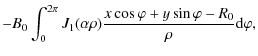
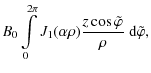
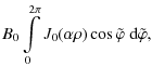
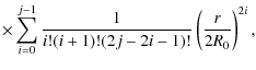
The ``total'' magnetic field
![$\displaystyle B_0 \int_0^{2\pi} \left[{J}_1 (\alpha\rho)
\frac{z \cos\varphi}{\rho}
-{J}_0 (\alpha\rho) \sin\varphi\right] {\rm d}\varphi ,$](/articles/aa/full_html/2009/19/aa11701-09/img22.png)
![$\displaystyle B_0 \int_0^{2\pi} \left[{J}_1 (\alpha\rho)
\frac{z \sin\varphi}{\rho}
+{J}_0 (\alpha\rho) \cos\varphi\right] {\rm d}\varphi ,$](/articles/aa/full_html/2009/19/aa11701-09/img23.png)
where
It is not obvious from Eqs. (7)-(9) that there
is a rotational symmetry with respect to the z axis, so the
magnetic components are functions only of two arguments,
![]() and z. Therefore we present the components in
the cylindrical coordinate system r,
and z. Therefore we present the components in
the cylindrical coordinate system r,
![]() ,
and z(which is identical to the Cartesian axis z and is a rotational
axis of the toroid). The Br component reads
,
and z(which is identical to the Cartesian axis z and is a rotational
axis of the toroid). The Br component reads
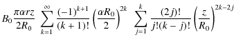
| Br | = | ||
| = | ![$\displaystyle B_0 \int\limits_0^{2\pi}
\left[{J}_1 (\alpha\rho) \frac{z \cos (\...
...hi-\phi)}{\rho}
-{J}_0 (\alpha\rho) \sin (\varphi-\phi)\right] {\rm d}\varphi ,$](/articles/aa/full_html/2009/19/aa11701-09/img29.png) |
where
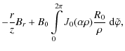
where
To integrate the formulae (10)-(12), we use
the definition for the Bessel function
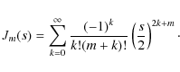
Applying the binomial formula twice for each component and using the identity for even powers of cosine (it is zero for odd powers)
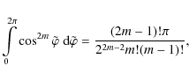
we get
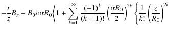
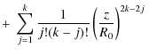
![$\displaystyle \times~ \Bigg[ 1 + \sum_{i=1}^{j}
\frac{(2j)!}{(i!)^2(2j-2i)!} \left(\frac{r}{2 R_0}\right)^{2i}
\Bigg] \Bigg\} \Bigg\rangle .$](/articles/aa/full_html/2009/19/aa11701-09/img46.png)
![\begin{figure}
\par\includegraphics[width=6.5cm,clip]{1701fig2.eps}
\end{figure}](/articles/aa/full_html/2009/19/aa11701-09/img47.png) |
Figure 2: Magnetic field distribution and field lines of toroidal flux ropes. The figures show cross sections through two flux ropes. The dashed circles are cross sections of generating toroids with aspect ratios of 2 a) and 4 b). |
| Open with DEXTER | |
3 Analysis of the new solution
Equations (15)-(17) represent an analytical solution for
a toroidal magnetic field which is exactly solenoidal and force-free
with constant ![]() for any aspect ratio. However, for numerical calculations it is more
suitable (and faster) to use expressions (7)-(9) or (10)-(12) directly; the series (13) can be reasonably
used for numerical purposes only with arguments up to |s|<8.
for any aspect ratio. However, for numerical calculations it is more
suitable (and faster) to use expressions (7)-(9) or (10)-(12) directly; the series (13) can be reasonably
used for numerical purposes only with arguments up to |s|<8.
Figure 2 shows magnetic field distributions of the new solution and
several magnetic field lines for two aspect ratios. The constant
![]() in the formulae (7)-(9) was set to
in the formulae (7)-(9) was set to
![]() (see the text above on the Lundquist solution). The field
has an azimuthal symmetry, so the distribution is displayed only in
one plane, y=0. Of course, the field is defined over all the
plane, but distributions in the figures are restricted only to
regions forming simple flux ropes (for clearness). So the
distributions represent cross sections through the toroidal flux
ropes. Magnetic field lines have helical forms and are defined by
(see the text above on the Lundquist solution). The field
has an azimuthal symmetry, so the distribution is displayed only in
one plane, y=0. Of course, the field is defined over all the
plane, but distributions in the figures are restricted only to
regions forming simple flux ropes (for clearness). So the
distributions represent cross sections through the toroidal flux
ropes. Magnetic field lines have helical forms and are defined by
![]() Each shown closed line may form a boundary
of a toroidal flux rope. Flux ropes do not have a circular cross
section, it is prolate and tear-drop like for larger aspect ratios.
This means that the solution does not tend to the Lundquist-type
solution for large aspect ratios. On the other hand, profiles of
magnetic field components are similar to the Lundquist solution.
This is shown in Fig. 3. The profiles are scaled by the respective
maximum value
Each shown closed line may form a boundary
of a toroidal flux rope. Flux ropes do not have a circular cross
section, it is prolate and tear-drop like for larger aspect ratios.
This means that the solution does not tend to the Lundquist-type
solution for large aspect ratios. On the other hand, profiles of
magnetic field components are similar to the Lundquist solution.
This is shown in Fig. 3. The profiles are scaled by the respective
maximum value
![]() of the field in the ropes (therefore
each B-plot in the top panel reaches a value of 1). The Lundquist
solution is displayed for comparison by dotted lines and its
profiles are shifted so that its B-maximum is close to B-maxima
of the displayed flux ropes. B-maximum, which is shifted towards
the toroid's hole from the flux-rope axis, becomes closer to the
axis for larger aspect ratios.
of the field in the ropes (therefore
each B-plot in the top panel reaches a value of 1). The Lundquist
solution is displayed for comparison by dotted lines and its
profiles are shifted so that its B-maximum is close to B-maxima
of the displayed flux ropes. B-maximum, which is shifted towards
the toroid's hole from the flux-rope axis, becomes closer to the
axis for larger aspect ratios.
![\begin{figure}
\par\includegraphics[width=7.5cm,clip]{1701fig3.eps}
\end{figure}](/articles/aa/full_html/2009/19/aa11701-09/img50.png) |
Figure 3: Profiles of the magnetic field magnitude B and magnetic field components By and Bz through the flux ropes shown in Fig. 2. They are profiles along the x-axis, the solid line is for the flux rope with R0/r0 = 2 and the dashed line for R0/r0 = 4. The dotted line shows the Lundquist solution for comparison. The Bx component is not displayed because it is zero for all the cases. The profiles are scaled by the respective maximum value of B in the plot. |
| Open with DEXTER | |
4 Modification of the solution
The presented solution has one shortfall in its application to interpretation of interplanetary flux ropes, namely a prolate shape. It is known that interplanetary flux ropes are oblate (Russell et al. 2002; Hu & Sonnerup 2002; Hidalgo et al. 2002; Vandas et al. 2005). To treat this case, we apply our solution of a linear force-free field in an elliptic cylinder (Vandas & Romashets 2003) and use it in the procedure described in Sect. 2. Insted of circular cylinders, elliptic cylinders are involved with the semiminor axis (b = r0) along the y'-axis (Fig. 1) and the semimajor axis (a) along the x'-axis. The linear force-free solution in elliptic cylindrical coordinates reads
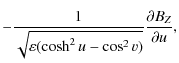
where
and
Following the procedure described in the previous section, the field (18)-(20) is expressed in the local Cartesian
coordinates
(x',y',z') in analogy to Eqs. (4)-(6),
then transformed into the global system (x,y,z) and integrated
over ![]() (similarly to Eqs. (7)-(9)). The
resulting field is a linear force-free field, because the generating
field (18)-(20) is, also for arbitrary aspect ratio and
oblateness. Due to the complexity of the transformations and the
presence of special functions, the whole procedure is implemented
numerically for field determination.
(similarly to Eqs. (7)-(9)). The
resulting field is a linear force-free field, because the generating
field (18)-(20) is, also for arbitrary aspect ratio and
oblateness. Due to the complexity of the transformations and the
presence of special functions, the whole procedure is implemented
numerically for field determination.
Figure 4 shows magnetic field distributions and several magnetic field
lines in a similar way as in Fig. 2; in addition to aspect ratios,
there is a new parameter, oblateness of the generating ellipse a/b. One can see how the shape of flux ropes changes with
oblateness. In fact, there is a smooth transition of shapes from the
one shown in Fig. 2b into those shown in Fig. 4, because the
solution (1)-(3) is a limiting case of
Eqs. (18)-(20) for
![]() .
Figure 4 also
demonstrates that B-maxima are shifted towards the toroid's hole
from the flux-rope axis, in accordance with Fig. 2.
.
Figure 4 also
demonstrates that B-maxima are shifted towards the toroid's hole
from the flux-rope axis, in accordance with Fig. 2.
5 Conclusions
Exact linear force-free magnetic field distributions in toroidal geometry were derived. Originally we intended them for the interpretation of interplanetary magnetic clouds and solar flux ropes, but they can be applied to laboratory plasma and astrophysical objects as well.
![\begin{figure}
\par\includegraphics[width=9cm,clip]{1701fig4.eps}
\end{figure}](/articles/aa/full_html/2009/19/aa11701-09/img64.png) |
Figure 4: Magnetic field distribution and field lines of toroidal flux ropes. The figures show cross sections through two flux ropes. The layout is the same as in Fig. 2. The dashed ellipses are cross sections of generating toroids with aspect ratios/oblatenesses of 4/1.25 a) and 4/2 b). |
| Open with DEXTER | |
Acknowledgements
The authors wish to express sincere thanks to many colleagues for useful discussions. This work was supported by the program of the Czech-US collaboration in science and technology (ME09032). In addition, E.R. was supported by a BELSPO fellowship and M.V. by the AV CR project 1QS300120506 and by the GA CR grant 205/09/0170.
References
- Burlaga, L. F. 1988, J. Geophys. Res., 93, 7217 [NASA ADS] [CrossRef]
- Hidalgo, M. A., Nieves-Chinchilla, T., & Cid, C. 2002, Geophys. Res. Lett., 29, doi: 10.1029/2001GL013875 (In the text)
- Hollis, J. M., & Koupelis, T. 2000, ApJ, 528, 418 [NASA ADS] [CrossRef] (In the text)
- Hu, Q., & Sonnerup, B. U. Ö. 2002, J. Geophys. Res., 107, doi: 10.1029/2001JA000293 (In the text)
- Ivanov, K. G., Harshiladze, A. F., Eroshenko, E. G., & Stiazhkin, V. A. 1989, Sol. Phys., 120, 407 [NASA ADS] [CrossRef] (In the text)
- Klein, L. W., & Burlaga, L. F. 1982, J. Geophys. Res., 87, 613 [NASA ADS] [CrossRef]
- Lepping, R. P., Burlaga, L. F., & Jones, J. A. 1990, J. Geophys. Res., 95, 11957 [NASA ADS] [CrossRef] (In the text)
- Lepping, R. P., Berdichevsky, D. B., Wu, C.-C., et al. 2006, Ann. Geophys., 24, 215 [NASA ADS] (In the text)
- Lundquist, S. 1950, Ark. Fys., 2, 361 (In the text)
- Marubashi, K. 1997, in Coronal Mass Ejections, ed. N. Crooker, J. Joselyn, & J. Feyman (Washington, D. C.: AGU), Geophys. Monogr. Ser., 99, 147 (In the text)
- Marubashi, K., & Lepping, R. P. 2007, Ann. Geophys., 25, 2453 [NASA ADS] (In the text)
- Miller, G., & Turner, L. 1981, Phys. Fluids, 24, 363 [NASA ADS] [CrossRef] (In the text)
- Ragland, S., Le Coroller, H., Pluzhnik, et al. 2008, ApJ, 679, 746 [NASA ADS] [CrossRef] (In the text)
- Romashets, E. P., & Vandas, M. 2003a, Geophys. Res. Lett., 30, doi: 10.1029/2003GL017692 (In the text)
- Romashets, E. P., & Vandas, M. 2003b, in Proc. ISCS 2003 Symposium, Solar Variability as an Input to the Earth's Environment, ESA SP-535, ed. A. Wilson (Noordwijk: ESTEC), 535
- Russell, C. T., & Mulligan, T. 2002, Planet. Space Sci., 50, 527 [NASA ADS] [CrossRef] (In the text)
- Vandas, M., & Romashets, E. P. 2003, A&A, 398, 801 [NASA ADS] [CrossRef] [EDP Sciences] (In the text)
- Vandas, M., Odstrcil, D., & Watari, S. 2002, J. Geophys. Res., 107, doi: 10.1029/2001JA005068 (In the text)
- Vandas, M., Romashets, E., & Watari, S. 2005, Planet. Space Sci., 53, 19 [NASA ADS] [CrossRef] (In the text)
All Figures
| |
Figure 1: Construction of a toroidal solution. |
| Open with DEXTER | |
| In the text | |
| |
Figure 2: Magnetic field distribution and field lines of toroidal flux ropes. The figures show cross sections through two flux ropes. The dashed circles are cross sections of generating toroids with aspect ratios of 2 a) and 4 b). |
| Open with DEXTER | |
| In the text | |
| |
Figure 3: Profiles of the magnetic field magnitude B and magnetic field components By and Bz through the flux ropes shown in Fig. 2. They are profiles along the x-axis, the solid line is for the flux rope with R0/r0 = 2 and the dashed line for R0/r0 = 4. The dotted line shows the Lundquist solution for comparison. The Bx component is not displayed because it is zero for all the cases. The profiles are scaled by the respective maximum value of B in the plot. |
| Open with DEXTER | |
| In the text | |
| |
Figure 4: Magnetic field distribution and field lines of toroidal flux ropes. The figures show cross sections through two flux ropes. The layout is the same as in Fig. 2. The dashed ellipses are cross sections of generating toroids with aspect ratios/oblatenesses of 4/1.25 a) and 4/2 b). |
| Open with DEXTER | |
| In the text | |
Copyright ESO 2009
Current usage metrics show cumulative count of Article Views (full-text article views including HTML views, PDF and ePub downloads, according to the available data) and Abstracts Views on Vision4Press platform.
Data correspond to usage on the plateform after 2015. The current usage metrics is available 48-96 hours after online publication and is updated daily on week days.
Initial download of the metrics may take a while.