| Issue |
A&A
Volume 498, Number 2, May I 2009
|
|
|---|---|---|
| Page(s) | 575 - 589 | |
| Section | Planets and planetary systems | |
| DOI | https://doi.org/10.1051/0004-6361/200811305 | |
| Published online | 18 February 2009 | |
Terrestrial planet formation in low-eccentricity warm-Jupiter systems
M. J. Fogg - R. P. Nelson
Astronomy Unit, Queen Mary, University of London, Mile End Road, London E1 4NS, UK
Received 7 November 2008 / Accepted 30 January 2009
Abstract
Context. Extrasolar giant planets are found to orbit their host stars with a broad range of semi-major axes
![]() AU. Current theories suggest that giant planets orbiting at distances between
AU. Current theories suggest that giant planets orbiting at distances between
![]() AU probably formed at larger distances and migrated to their current locations via type II migration, disturbing any inner system of forming terrestrial planets along the way. Migration probably halts because of fortuitously-timed gas disk dispersal.
AU probably formed at larger distances and migrated to their current locations via type II migration, disturbing any inner system of forming terrestrial planets along the way. Migration probably halts because of fortuitously-timed gas disk dispersal.
Aims. The aim of this paper is to examine the effect of giant planet migration on the formation of inner terrestrial planet systems. We consider situations in which the giant planet halts migration at semi-major axes in the range 0.13-1.7 AU due to gas disk dispersal, and examine the effect of including or neglecting type I migration forces on the forming terrestrial system.
Methods. We employ an N-body code that is linked to a viscous gas disk algorithm capable of simulating gas loss via accretion onto the central star and photoevaporation, gap formation by the giant planet, type II migration of the giant, optional type I migration of protoplanets, and gas drag on planetesimals.
Results. Most of the inner system planetary building blocks survive the passage of the giant planet, either by being shepherded inward or scattered into exterior orbits. Systems of one or more hot-Earths are predicted to form and remain interior to the giant planet, especially if type II migration has been limited, or where type I migration has affected protoplanetary dynamics. Habitable planets in low-eccentricity warm-Jupiter systems appear possible if the giant planet makes a limited incursion into the outer regions of the habitable zone (HZ), or traverses its entire width and ceases migrating at a radial distance of less than half that of the HZ's inner edge.
Conclusions. Type II migration does not prevent terrestrial planet formation. A wide variety of planetary system architectures exists that can potentially host habitable planets.
Key words: planets and satellites: formation - methods: N-body simulations - astrobiology
1 Introduction
Giant planets are thought to form in the cool, outer, regions of a
protoplanetary disk (e.g. Papaloizou & Nelson 2005; Boss 2000; Pollack et al. 1996), in
roughly the region where Jupiter and Saturn are found in our solar
system. However, numerous giant exoplanets have been found orbiting
solar-type stars well inside the approximate position of their
nebular snowline with semi-major axes from ![]() 3 AU down to just
a few stellar radii (Butler et al. 2006). The most extreme examples of
these are the so-called ``hot-Jupiters'', orbiting within 0.1 AU and
accounting for about a quarter of the known giant exoplanet
inventory. Planetary migration may provide the best explanation for
the presence of the hot-Jupiter population, in particular type II
migration, where the giant planet has grown massive enough to open a
gap in its protoplanetary disk and migrates inward in step with the
disk's viscous evolution (e.g. Lin & Papaloizou 1986; Nelson et al. 2000; Lin et al. 1996; Ward 1997).
Giant exoplanets at intermediate distances, where eccentricities can
be high, might be explained by mutual scattering
of giant planets (e.g. Marzari & Weidenschilling 2002; Ford et al. 2001; Papaloizou & Terquem 2001; Lin & Ida 1997),
a combination of migration and scattering (Moorhead & Adams 2005; Adams & Laughlin 2003),
or migration along with eccentricity excitation from the disk
(Papaloizou et al. 2001; Ogilvie & Lubow 2003; Moorhead & Adams 2008; Goldreich & Sari 2003).
3 AU down to just
a few stellar radii (Butler et al. 2006). The most extreme examples of
these are the so-called ``hot-Jupiters'', orbiting within 0.1 AU and
accounting for about a quarter of the known giant exoplanet
inventory. Planetary migration may provide the best explanation for
the presence of the hot-Jupiter population, in particular type II
migration, where the giant planet has grown massive enough to open a
gap in its protoplanetary disk and migrates inward in step with the
disk's viscous evolution (e.g. Lin & Papaloizou 1986; Nelson et al. 2000; Lin et al. 1996; Ward 1997).
Giant exoplanets at intermediate distances, where eccentricities can
be high, might be explained by mutual scattering
of giant planets (e.g. Marzari & Weidenschilling 2002; Ford et al. 2001; Papaloizou & Terquem 2001; Lin & Ida 1997),
a combination of migration and scattering (Moorhead & Adams 2005; Adams & Laughlin 2003),
or migration along with eccentricity excitation from the disk
(Papaloizou et al. 2001; Ogilvie & Lubow 2003; Moorhead & Adams 2008; Goldreich & Sari 2003).
In the case of migrating planets, the mechanism that terminates the
migration and strands exoplanets at their present orbital radii is
unknown. Migration-halting mechanisms that might work when the
planet ventures close to the central star include tidally-induced
recession caused by the star's rotation or Roche lobe overflow and
mass loss to the star (Trilling et al. 1998), or intrusion by the planet
into a central cavity or surface density transition in the disk,
decoupling it from the evolution of the gas
(Lin et al. 1996; Kuchner & Lecar 2002; Masset et al. 2006; Papaloizou 2007). Halting migration further
out, beyond the ![]() 0.1 AU hot-Jupiter region, may require
that giant planets form late in the lifetime of the gas disk and
hence only have time for a partial inward migration before stranding
at an intermediate distance when the gas is lost (Trilling et al. 1998).
Disks around T Tauri stars are observed to last for
0.1 AU hot-Jupiter region, may require
that giant planets form late in the lifetime of the gas disk and
hence only have time for a partial inward migration before stranding
at an intermediate distance when the gas is lost (Trilling et al. 1998).
Disks around T Tauri stars are observed to last for ![]() 1-10 Myr (Haisch et al. 2001) but disperse over a much shorter
1-10 Myr (Haisch et al. 2001) but disperse over a much shorter ![]() 105 year timescale (Wolk & Walter 1996; Simon & Prato 1995): a behaviour that may result
primarily by accretion of gas onto the central star combined with
photoevaporative gas loss driven by the stellar UV output
(Alexander et al. 2006; Clarke et al. 2001). Models of this stranding mechanism
(Armitage et al. 2002; Armitage 2007), which can roughly reproduce the
exoplanet semi-major axis statistics, have raised the possibility
that fortuitous disk dispersal might also explain the presence of
the hot-Jupiter population and imply that earlier formed giant
planets could have been consumed by the cental star.
105 year timescale (Wolk & Walter 1996; Simon & Prato 1995): a behaviour that may result
primarily by accretion of gas onto the central star combined with
photoevaporative gas loss driven by the stellar UV output
(Alexander et al. 2006; Clarke et al. 2001). Models of this stranding mechanism
(Armitage et al. 2002; Armitage 2007), which can roughly reproduce the
exoplanet semi-major axis statistics, have raised the possibility
that fortuitous disk dispersal might also explain the presence of
the hot-Jupiter population and imply that earlier formed giant
planets could have been consumed by the cental star.
If type II migration correctly accounts for the presence of the hot-Jupiter population then these giant planets must have traversed their inner systems at a time when gas was still present and before the completion of terrestrial planet formation. This prompted initial speculations that such systems would be likely to lack any terrestrial planets within their inner few AU (Armitage 2003), and since hot-Jupiters are not uncommon, they have been used to infer significant constraints on the abundance of habitable planets (Ward & Brownlee 2000), and even their galactic location (Lineweaver et al. 2004; Lineweaver 2001). This view is contradicted however by recent models that have simulated the process of a giant planet migrating through an interior protoplanetary disk (Fogg & Nelson 2005; Raymond et al. 2006; Fogg & Nelson 2007b,2006; Mandell et al. 2007; Fogg & Nelson 2007a). These find that solid material is not predominantly accreted by the giant planet or the central star; instead, solid bodies captured at interior mean motion resonances with the giant are shepherded inward an arbitrary distance before being randomly scattered into an external orbit. The net result after the migration is a partitioning of most of the original disk material into two remnants: a compacted remnant interior to the final orbit of the giant, which typically accretes in a short timescale to form hot-Earth or hot-Neptune planets; and an external disk of scattered bodies. The relative predominance of these outcomes has been shown to be sensitive to the strength of dissipative forces operating at the time of migration (Fogg & Nelson 2005,2007b,a) with scattering becoming increasingly prevalent in late migration scenarios when less gas is present. All these studies concur that a scattered disk of sufficient mass to support renewed planet formation is likely to be generated under a variety of conditions and that terrestrial planets should be commonplace in hot-Jupiter systems, rather than rare or absent.
One simplification common to these previous models is that the physical mechanism that actually halts giant planet migration is not specified or modeled. Type II migration is artificially halted when the giant planet has reached a preset final orbit and hence is not determined by the structure or evolution of the gas disk. Since these models stop migration close to the central star, whilst significant gas is still present, they appear most realistic in the context of a central gaseous cavity halting mechanism. The examples that come closest to implicitly assuming fortuitous gas disk dispersal as the halting mechanism are the late scenarios of Fogg & Nelson (2007b,a) where gas densities have fallen to low levels and migration is decelerating (see Fig. 3 in Fogg & Nelson 2007a, and Fig. 3 of this paper). However, the final hot-Jupiter orbits in these papers are still artificially imposed at 0.1 AU and are not controlled self-consistently by the evolution of the gas.
Our previous model adopted a 1-D, viscously evolving, gas disk
algorithm which simulates accretion onto the central star, annular
gap formation in the vicinity of a giant planet, and self-consistent
type II migration; for the nebular parameters chosen, the mass of
our gas disk exponentially declined with an e-folding time of
582 000 years (Fogg & Nelson 2007a). This sort of model runs into trouble
when simulating the late stages of gas disk dispersal as it does not
reproduce a final and abrupt ![]() 105 year decline that would
accord with observations. We have corrected this deficiency here by
including a photoevaporation algorithm in our code that gradually
erodes and removes mass from our gas disk. As shown by
Clarke et al. (2001) and Alexander et al. (2006), this process has little effect
on the evolution and structure of the gas disk at early times, but
comes to dominate at later times once the rate of gas loss onto the
central star due to viscous evolution
falls below the photoevaporation rate. A rapid
dispersal of the remaining gas follows, along with the cessation of
any ongoing giant planet migration.
105 year decline that would
accord with observations. We have corrected this deficiency here by
including a photoevaporation algorithm in our code that gradually
erodes and removes mass from our gas disk. As shown by
Clarke et al. (2001) and Alexander et al. (2006), this process has little effect
on the evolution and structure of the gas disk at early times, but
comes to dominate at later times once the rate of gas loss onto the
central star due to viscous evolution
falls below the photoevaporation rate. A rapid
dispersal of the remaining gas follows, along with the cessation of
any ongoing giant planet migration.
In this paper, we report on the results of a set of scenarios where
giant planet stranding distances are no longer prescribed but which
happen when migration runs out of steam at the time of the
disappearance of the nebular gas. We therefore specifically assume
and self-consistently model fortuitous gas disk dispersal as
the mechanism that finalizes giant planets in their post-migration
orbits. Terrestrial planetary formation in this context is of
interest because, for a hot-Jupiter to strand at ![]() 0.1 AU, it
must form and migrate late in the lifetime of the gas disk, when gas
densities are lower and accretion in the inner system is at a more
advanced stage than previously considered. In addition, a succession
of later scenarios than this results in a succession of shorter
migrations and larger stranding distances. This has allowed us to
extend the scope of our study to model terrestrial planet growth in
those ``warm-Jupiter'' systems that may have originated as the result
of a late, partial, inward migration. In this paper we define
a ``warm-Jupiter'' to be one orbiting with semi-major axis in
the range
0.1 < a < 2.7 AU, where the outer limit coincides
with the snowline.
0.1 AU, it
must form and migrate late in the lifetime of the gas disk, when gas
densities are lower and accretion in the inner system is at a more
advanced stage than previously considered. In addition, a succession
of later scenarios than this results in a succession of shorter
migrations and larger stranding distances. This has allowed us to
extend the scope of our study to model terrestrial planet growth in
those ``warm-Jupiter'' systems that may have originated as the result
of a late, partial, inward migration. In this paper we define
a ``warm-Jupiter'' to be one orbiting with semi-major axis in
the range
0.1 < a < 2.7 AU, where the outer limit coincides
with the snowline.
The plan of the paper is as follows. In Sect. 2 we outline the additions to our model and the initial conditions of the simulations; in Sect. 3 the results are presented and discussed; in Sect. 4 we consider some caveats, and in Sect. 5 we offer our conclusions.
2 Description of the model
We model our systems using an enhanced version of the Mercury 6 hybrid-symplectic integrator (Chambers 1999), run as an N + N' body simulation, where there are N protoplanets embedded in a swarm of N' ``super-planetesimals'' - tracer particles with masses a tenth of the initial masses of protoplanets that act as an idealized ensemble of a much larger number of real planetesimals and are capable of exerting dynamical friction on larger bodies (e.g. Thommes et al. 2003). The central star, giant planet, and protoplanets interact gravitationally and can accrete and merge inelastically with all other bodies. Super-planetesimals however are non-self-interacting but subject to a drag force from their motion relative to the nebular gas that is equivalent to the gas drag that would be experienced by a single 10 km radius planetesimal. Details of these aspects of our model are given in Fogg & Nelson (2005).
We calculate the evolution of the nebular gas using a 1-D viscous
disk model that solves numerically a modified viscous gas disk
diffusion equation that includes the tidal torques exerted by an
embedded giant planet (Lin & Papaloizou 1986; Takeuchi et al. 1996) and have described its
implementation in Fogg & Nelson (2007a). The gas responds by depleting over
time via viscous accretion onto the central star; opening up an
annular gap centred on the giant planet's orbit; and forming a
partial inner cavity due to dissipation of propagating spiral waves
excited by the giant planet. The back reaction of these effects on
the giant planet is resolved as torques which self-consistently
drive type II migration. We model the possible effects of type I
migration (Cresswell & Nelson 2006; Tanaka & Ward 2004; Tanaka et al. 2002; Papaloizou & Larwood 2000; Ward 1997),
where a tidal interaction with the gas disk is thought to exert an
inward radial drift and strong eccentricity and inclination damping
on protoplanets of ![]()
![]() ,
using a simple
algorithm described in Fogg & Nelson (2007b).
,
using a simple
algorithm described in Fogg & Nelson (2007b).
As well as modeling the dynamics of gaseous volatiles in our model, we also track the movement of presumed solid volatiles, such as water ice and hydrated minerals, by labeling all particles with a composition based on their original location in the disk and summing the composition of protoplanets as they grow. We assume a crude three-phase initial radial composition with rocky material originating at <2 AU, material similar to chondritic meteorites between 2-2.7 AU, and trans-snowline material at >2.7 AU. We do not assign an actual water mass fraction to these phases.
2.1 Photoevaporation-driven disk dispersal
A gas disk that viscously drains onto its central star undergoes a
power law decline with a long drawn out dispersal in conflict with
observations that final dispersal occurs over a timescale that is
short compared with the disk age. Clarke et al. (2001) showed that this
could be explained by including a model of photoevaporation of the
disk driven by the diffuse UV flux from the central star
(Hollenbach et al. 1994). Their results show that once the accretion rate
onto the star declines to roughly equal the outer disk
photoevaporation rate, the inner disk ceases to be resupplied from
larger radii and rapidly drains onto the star. The formation of this
inner cavity then permits direct UV illumination of the outer disk
which disperses in turn in ![]() 105 years (Alexander et al. 2006).
105 years (Alexander et al. 2006).
For our purposes we need only adopt a simple parameterization of
this type of photoevaporation model and subtract from the right hand
side of our disk diffusion equation (Eq. (7) in Fogg & Nelson (2007a)) an
extra term representing a disk wind:
where
To fit with our pre-existing viscous gas disk model, we take
In Fogg & Nelson (2007b,a) we assumed an initial condition of a minimum
mass solar nebula model (Hayashi 1981), scaled up in mass by a
factor of three (3 ![]() MMSN), extending between 0.025-33 AU
from a solar mass protostar, with an initial surface density profile
of
MMSN), extending between 0.025-33 AU
from a solar mass protostar, with an initial surface density profile
of
![]() and a total mass of
0.039
and a total mass of
0.039 ![]() .
Having chosen an alpha viscosity of
.
Having chosen an alpha viscosity of
![]() ,
we found that, after a short lived
,
we found that, after a short lived ![]() 105 year period where
105 year period where
![]() close to the star
relaxes to a shallower profile, the mass of the gas disk declines
predictably with an e-folding time of 582 000 years. This behaviour
is illustrated as the upper blue curve in the top panel of
Fig. 1, which plots the nebular mass vs. time, and is
compared with the red curve which illustrates the effect of
including photoevaporation. It is evident that the two models only
diverge slowly for the first
close to the star
relaxes to a shallower profile, the mass of the gas disk declines
predictably with an e-folding time of 582 000 years. This behaviour
is illustrated as the upper blue curve in the top panel of
Fig. 1, which plots the nebular mass vs. time, and is
compared with the red curve which illustrates the effect of
including photoevaporation. It is evident that the two models only
diverge slowly for the first ![]() 2 Myr, but thereafter the mass
of the photoevaporating disk drops steeply and vanishes in just a
few
2 Myr, but thereafter the mass
of the photoevaporating disk drops steeply and vanishes in just a
few
![]() years. The lower panel of Fig. 1,
which plots the accretion rate onto the star
years. The lower panel of Fig. 1,
which plots the accretion rate onto the star
![]() ,
shows that this transition in behaviour
occurs around the time when
,
shows that this transition in behaviour
occurs around the time when
![]() .
.
![\begin{figure}
\par\includegraphics[width=7.5cm,clip]{11305fig1.eps}
\end{figure}](/articles/aa/full_html/2009/17/aa11305-08/img38.gif) |
Figure 1:
Upper panel: mass of the nebular gas vs. time: the blue curve
represents our former model where mass loss occurs solely via
viscous accretion onto the central star; the red curve
represents our new model including photoevaporation. Lower panel:
accretion rate onto the central star
|
| Open with DEXTER | |
![\begin{figure}
\par\includegraphics[width=7.5cm,clip]{figures_recadrées/11305fig2.eps}
\end{figure}](/articles/aa/full_html/2009/17/aa11305-08/img39.gif) |
Figure 2: Model gas disk surface density evolution. The uppermost curve is the initial condition; successive curves are labeled with their age in Myr. |
| Open with DEXTER | |
The evolution of the gas disk surface density
![]() is shown in Fig. 2, where
the uppermost curve represents the initial
is shown in Fig. 2, where
the uppermost curve represents the initial
![]() profile and the lower curve represent successively
more evolved configurations. It can be seen that the evolution of
the nebula speeds up after
profile and the lower curve represent successively
more evolved configurations. It can be seen that the evolution of
the nebula speeds up after ![]() 2 Myr, with a gap at
2 Myr, with a gap at
![]() starting to open up at
starting to open up at ![]() 2.38 Myr, followed by an
accelerated decline of the inner disk thereafter. This behaviour is
qualitatively similar to that described by Clarke et al. (2001), with the
exception that at late times our outer disk, which is truncated to a
much smaller radius, is lost even more rapidly. This makes no
difference to our mechanism for stranding giant planets as the
divergence occurs when the nebular mass has already fallen below the
level where it can drive migration. If giant planets strand well
inward of
2.38 Myr, followed by an
accelerated decline of the inner disk thereafter. This behaviour is
qualitatively similar to that described by Clarke et al. (2001), with the
exception that at late times our outer disk, which is truncated to a
much smaller radius, is lost even more rapidly. This makes no
difference to our mechanism for stranding giant planets as the
divergence occurs when the nebular mass has already fallen below the
level where it can drive migration. If giant planets strand well
inward of ![]() we found that they can act against the
efficient draining of the last dregs of the inner disk onto the
central star, slightly altering the picture given in
Fig. 2. Again however, this effect is minor as it
occurs at times when the gas is very thin and does not significantly
delay the date of overall disk dispersal.
we found that they can act against the
efficient draining of the last dregs of the inner disk onto the
central star, slightly altering the picture given in
Fig. 2. Again however, this effect is minor as it
occurs at times when the gas is very thin and does not significantly
delay the date of overall disk dispersal.
2.2 Initial conditions and running of the simulations
We do not consider the earliest stages of planetesimal formation and
runaway growth in our modeled systems and set the t = 0 start date
for our simulations to be 0.5 Myr after the start of star formation.
By this time, we assume that there is no more infall of gas onto the
protoplanetary disk and the solids component of the inner disk has
reached its oligarchic growth stage, where a succession of
protoplanets, each being a few percent of an Earth-mass, have
emerged from the planetesimal swarm in near-circular orbits and with
roughly equidistant spacing in units of mutual Hill radii
(Kokubo & Ida 2000). We assume a central star of 1.0
![]() with initial surface density profiles for gas and solids (
with initial surface density profiles for gas and solids (
![]() )
taken from a minimum mass solar nebular model
(Hayashi 1981), which is scaled up in mass by a factor of three
(3
)
taken from a minimum mass solar nebular model
(Hayashi 1981), which is scaled up in mass by a factor of three
(3 ![]() MMSN) to provide enough mass beyond the nebular snowline
for a giant planet to form before the loss of the nebular gas
(Thommes et al. 2003; Lissauer 1987). We model the gas component of the
protoplanetary disk between 0.025-33 AU, giving an initial mass
of 0.039
MMSN) to provide enough mass beyond the nebular snowline
for a giant planet to form before the loss of the nebular gas
(Thommes et al. 2003; Lissauer 1987). We model the gas component of the
protoplanetary disk between 0.025-33 AU, giving an initial mass
of 0.039 ![]() ,
and compute its evolution with our
photoevaporating viscous gas disk algorithm, as described in the
previous section and in Fogg & Nelson (2007a). We take the alpha viscosity
of the gas to be
,
and compute its evolution with our
photoevaporating viscous gas disk algorithm, as described in the
previous section and in Fogg & Nelson (2007a). We take the alpha viscosity
of the gas to be
![]() ,
which gives a viscous
evolution time at 5 AU
,
which gives a viscous
evolution time at 5 AU ![]() 120 000 years.
120 000 years.
Table 1: Data describing initial solids disk set-up.
We model the solids component of the disk initially between 0.4-5.0 AU and assume a snowline at 2.7 AU beyond which
the mass of solids is boosted by a
factor of 4.2 by the condensation of ices.
We generate the initial N-body components of the solids disk
in an identical manner to that detailed in Fogg & Nelson (2005) by starting
with initial protoplanetary masses of 0.025 and
0.1
![]() interior and exterior to the snowline
respectively, spaced approximately 8 mutual Hill radii apart, with
the remainder of the material inventory consisting of
super-planetesimals with a fixed mass of 10% of the initial masses
of the local protoplanets. Relevant data for the initial solids
components are shown in Table 1 which gives, for zones
interior and exterior to the snowline, values for the total mass of
solid material
interior and exterior to the snowline
respectively, spaced approximately 8 mutual Hill radii apart, with
the remainder of the material inventory consisting of
super-planetesimals with a fixed mass of 10% of the initial masses
of the local protoplanets. Relevant data for the initial solids
components are shown in Table 1 which gives, for zones
interior and exterior to the snowline, values for the total mass of
solid material
![]() ,
the number and mass of
protoplanets N and
,
the number and mass of
protoplanets N and
![]() ,
and the number and mass
of super-planetesimals N' and
,
and the number and mass
of super-planetesimals N' and
![]() .
The parameter
.
The parameter
![]() ,
at the foot of Table 1, is the mass
fraction of the solids disk contained in protoplanets and we use
this here as a rough measure of the evolution of the disk, taking
,
at the foot of Table 1, is the mass
fraction of the solids disk contained in protoplanets and we use
this here as a rough measure of the evolution of the disk, taking
![]() to denote the transition between oligarchic
and chaotic, or ``giant impact'', growth regimes (Goldreich et al. 2004).
to denote the transition between oligarchic
and chaotic, or ``giant impact'', growth regimes (Goldreich et al. 2004).
Our previous approach was to run our combined N-body and gas disk
model, in the absence of a giant planet, from t = 0 to a set of
durations distributed between 0.1-1.5 Myr, in order to mature the
disk to different ages and to generate a set of migration scenarios.
At the end of each of these maturation runs, we then introduced a
0.5 MJ giant planet at 5 AU, after removing
0.4 MJ of gas from a local disk annulus to provide for
the giant planet's envelope. This gas is assumed to have accreted on
top of a 0.1 MJ solid core, composed of material
deriving from beyond the outer boundary of our modelled solids disk.
Re-starting the run at this point resulted in an inward type II
migration of the giant planet which was allowed to continue until it
reached our prescribed stranding radius of 0.1 AU. This approach is
not appropriate here as we are specifically assuming gas disk
dispersal as the stranding mechanism and therefore need to mature
the disk to between the boundaries of a temporal window within which
our giant planet can both accrete sufficient gas for its envelope
and cease migration at ![]() 0.1 AU. We located the lower limit
of this window, the age where a 0.5 MJ giant planet
introduced at 5 AU will naturally cease migrating and come to rest
at
0.1 AU. We located the lower limit
of this window, the age where a 0.5 MJ giant planet
introduced at 5 AU will naturally cease migrating and come to rest
at ![]() 0.1 AU, via experiments with the model and found it to be
0.1 AU, via experiments with the model and found it to be
![]() Myr. By this time, the mass of the nebula has
fallen to
Myr. By this time, the mass of the nebula has
fallen to
![]() which is
shown as the upper dotted line in Fig. 1. The maximum
possible upper age limit of the stranding window would be when
which is
shown as the upper dotted line in Fig. 1. The maximum
possible upper age limit of the stranding window would be when
![]() ,
at
,
at
![]() Myr (see
the lower dotted line in Fig. 1), giving a window
duration of
Myr (see
the lower dotted line in Fig. 1), giving a window
duration of ![]()
![]() of the simulated disk lifetime. However,
this limit would require the unrealistic condition of all the
remaining nebular gas being accreted by the giant planet. Since we
do not simulate the process of gas accretion onto the giant planet's
core, we have arbitrarily restricted the upper age limit of the
stranding window to t = 1.85 Myr (see the middle dotted line in
Fig. 1) by which time the mass of the nebula has fallen
to
of the simulated disk lifetime. However,
this limit would require the unrealistic condition of all the
remaining nebular gas being accreted by the giant planet. Since we
do not simulate the process of gas accretion onto the giant planet's
core, we have arbitrarily restricted the upper age limit of the
stranding window to t = 1.85 Myr (see the middle dotted line in
Fig. 1) by which time the mass of the nebula has fallen
to
![]() ,
reducing the window
duration to
,
reducing the window
duration to ![]()
![]() of the simulated disk lifetime. We note that
the model of Armitage et al. (2002) predicts a stranding window of
duration
of the simulated disk lifetime. We note that
the model of Armitage et al. (2002) predicts a stranding window of
duration ![]()
![]() of the disk lifetime. This longer duration
compared to ours is because they adopted a more slowly evolving disk
model and were simulating the stranding of more massive giant
planets which migrate more slowly. Clearly, variation of the many
free parameters in a model such as this can produce a variety of
stranding behaviours in simulations, but we have not considered
these here as our main focus is on the effect that the giants'
stranding distances have on the partitioning of the inner system
disk and subsequent terrestrial planet formation.
of the disk lifetime. This longer duration
compared to ours is because they adopted a more slowly evolving disk
model and were simulating the stranding of more massive giant
planets which migrate more slowly. Clearly, variation of the many
free parameters in a model such as this can produce a variety of
stranding behaviours in simulations, but we have not considered
these here as our main focus is on the effect that the giants'
stranding distances have on the partitioning of the inner system
disk and subsequent terrestrial planet formation.
The behaviour of 0.5 MJ giant planets launched into our
model disks, between the lower and upper age limits discussed above,
is illustrated by the solid curves in Fig. 3 and shows
that stranding takes place between 0.13-1.71 AU. Also illustrated
by the dashed curves in Fig. 3 are the migration
trajectories of the giant planets in Scenarios III, IV, and V of
Fogg & Nelson (2007a) where migration takes place in a younger disk and was
artificially halted at 0.1 AU by a presumed inner disk cavity. The
fastest of these (launched at 0.5 Myr) takes place at a time when
the gas disk is still quite massive and completes its migration in
the viscous evolution time of ![]() 120 000 years. Later scenarios
entail longer migration times as the gas mass progressively declines
and is less effective at driving migration. In order for giant
planets to strand naturally, our present models require still later
launch times, in a context where photoevaporation is starting to
have a significant influence on the disk. Figure 3 shows
that migration speeds are considerably slower and decelerate
steadily until migration ceases after
120 000 years. Later scenarios
entail longer migration times as the gas mass progressively declines
and is less effective at driving migration. In order for giant
planets to strand naturally, our present models require still later
launch times, in a context where photoevaporation is starting to
have a significant influence on the disk. Figure 3 shows
that migration speeds are considerably slower and decelerate
steadily until migration ceases after
![]() years for the
farthest travelling planet and 470 000 years for the planet that
migrates the least. Migration in all these cases halts at
years for the
farthest travelling planet and 470 000 years for the planet that
migrates the least. Migration in all these cases halts at
![]() Myr
Myr![]() .
.
Thus, we generated the scenarios for this paper by running the model
from its initial condition, without a giant planet present, to
mature the protoplanetary disk to a minimum of t = 1.77 Myr and
then in successive 10 000 year increments to t = 1.85 Myr. Given
that the reality of strong type I migration is controversial, and to
bracket the range of possibilities, two parallel sets of scenarios
are generated: one with no type I migration forces (Run Set
A) and the other with type I migration and eccentricity and
inclination damping set at the maximum rate determined by
Eqs. (1) and (2) in Fogg & Nelson (2007b) (Run Set B). To accommodate
this total of 18 simulations, a change from our previous scenario ID
system is also required. Thus, Roman numerals are substituted with
Arabic numerals and labelling is generated by the following formula:
![]() .
This
gives Scenarios 1, 2, ..., 9 for t = 1.77, 1.78, ..., 1.85 Myr. Run
set B which includes type I migration is denoted by an I
subscript: e.g.
Scenarios
.
This
gives Scenarios 1, 2, ..., 9 for t = 1.77, 1.78, ..., 1.85 Myr. Run
set B which includes type I migration is denoted by an I
subscript: e.g.
Scenarios
![]() .
During
these maturation runs the simulation inner edge was set at 0.1 AU
and any material passing interior to this boundary was eliminated
and assumed to be consumed by the central star. The configuration of
these matured solids disks at t = 1.77 Myr, the opening of the
stranding window, are shown in Fig. 4 and
Table 2 gives relevant data including values for the
remaining total mass
.
During
these maturation runs the simulation inner edge was set at 0.1 AU
and any material passing interior to this boundary was eliminated
and assumed to be consumed by the central star. The configuration of
these matured solids disks at t = 1.77 Myr, the opening of the
stranding window, are shown in Fig. 4 and
Table 2 gives relevant data including values for the
remaining total mass
![]() ,
the maximum
protoplanetary mass
,
the maximum
protoplanetary mass
![]() ,
the numbers of surviving
protoplanets and super-planetesimals
,
the numbers of surviving
protoplanets and super-planetesimals
![]() ,
and the
protoplanet to whole disk mass fraction
,
and the
protoplanet to whole disk mass fraction
![]() .
Since
the scenarios of the present work start much closer together in time than
those of our previous models (0.01 Myr vs. 0.15-0.5 Myr), the
state of the solids disks generated for Scenarios 2-9 does not
change greatly from that of Scenario 1.
.
Since
the scenarios of the present work start much closer together in time than
those of our previous models (0.01 Myr vs. 0.15-0.5 Myr), the
state of the solids disks generated for Scenarios 2-9 does not
change greatly from that of Scenario 1.
![\begin{figure}
\par\includegraphics[width=7.5cm,clip]{11305fig3.eps}
\end{figure}](/articles/aa/full_html/2009/17/aa11305-08/img71.gif) |
Figure 3:
Migration and stranding of 0.5 MJ giant planets
in our present and previous models. Giant planet semi major axis in
AU is plotted against |
| Open with DEXTER | |
![\begin{figure}
\par\includegraphics[width=12cm,clip]{11305fig4.eps}
\end{figure}](/articles/aa/full_html/2009/17/aa11305-08/img72.gif) |
Figure 4: Eccentricity vs. semi-major axis for matured solids disks at 1.77 Myr for no type I migration ( top panel) and with type I migration ( bottom panel). Grey dots are super-planetesimals; red and blue circles are protoplanets originating interior and exterior to the snowline respectively. Gas densities are read on the right hand axes: the upper blue lines show gas density at t = 0 and the lower cyan lines are the current densities. |
| Open with DEXTER | |
It can be seen, when comparing with the initial condition data in
Table 1, that planetary growth has been strong,
especially where no type I migration is operating. In this case (the
upper panel in Fig. 4), mergers have reduced
protoplanets to a third of their former number,
![]() is high (there being a
is high (there being a
![]() planet present at 2.01 AU), and
planet present at 2.01 AU), and
![]() indicates that the accretion pattern of the disk has progressed way beyond oligarchic growth into
the chaotic growth regime. Very little mass has been lost interior
to 0.1 AU (
indicates that the accretion pattern of the disk has progressed way beyond oligarchic growth into
the chaotic growth regime. Very little mass has been lost interior
to 0.1 AU (![]()
![]() )
via dynamical spreading and gas drag induced
orbital decay of planetesimals. With type I migration, there is in
play an additional preferential damping and inward migration of the
most massive protoplanets (clearly visible in the lower panel in
Fig. 4) resulting in the loss of
)
via dynamical spreading and gas drag induced
orbital decay of planetesimals. With type I migration, there is in
play an additional preferential damping and inward migration of the
most massive protoplanets (clearly visible in the lower panel in
Fig. 4) resulting in the loss of ![]()
![]() of the
disk mass beyond the simulation inner edge. This loss is mostly in
the form of large bodies as can be inferred from the lower values of
of the
disk mass beyond the simulation inner edge. This loss is mostly in
the form of large bodies as can be inferred from the lower values of
![]() ,
N, and
,
N, and
![]() .
It might be thought
that this loss is quite modest considering our inclusion of type I
migration forces. However, in a rapidly dispersing gas disk model
such as ours, inward type I migration, which is proportional to
planetary mass, is limited at early times by the small size of
protoplanets, and at late times by low gas densities (see
also Daisaka et al. 2006; McNeil et al. 2005); Fig. 4 shows that at t =
1.77 Myr,
.
It might be thought
that this loss is quite modest considering our inclusion of type I
migration forces. However, in a rapidly dispersing gas disk model
such as ours, inward type I migration, which is proportional to
planetary mass, is limited at early times by the small size of
protoplanets, and at late times by low gas densities (see
also Daisaka et al. 2006; McNeil et al. 2005); Fig. 4 shows that at t =
1.77 Myr,
![]() interior to 1 AU has fallen by two
orders of magnitude. The effect of type I migration on the radial
distribution of solids disk mass is shown in Fig. 5
where the total solids mass for both models at t = 1.77 Myr is
plotted in 0.5 AU width bins against radial distance. It can be seen
that beyond
interior to 1 AU has fallen by two
orders of magnitude. The effect of type I migration on the radial
distribution of solids disk mass is shown in Fig. 5
where the total solids mass for both models at t = 1.77 Myr is
plotted in 0.5 AU width bins against radial distance. It can be seen
that beyond ![]() 2 AU the radial mass profile of the disks in the
two models remains similar, but interior to 2 AU the more rapid pace
of protoplanetary growth has resulted, in the type I migration case,
in an inward displacement of mass caused mainly by a fractionation
of the most massive bodies from the rest of the swarm which are now
crowding the inner 0.5 AU of the system. It was shown in
Fogg & Nelson (2007b) that hot-Earth type planets are more likely to accrete
and survive when a giant planet migrates through such a solids disk,
where previous type I migration has caused a radial contraction of
the inner mass distribution.
2 AU the radial mass profile of the disks in the
two models remains similar, but interior to 2 AU the more rapid pace
of protoplanetary growth has resulted, in the type I migration case,
in an inward displacement of mass caused mainly by a fractionation
of the most massive bodies from the rest of the swarm which are now
crowding the inner 0.5 AU of the system. It was shown in
Fogg & Nelson (2007b) that hot-Earth type planets are more likely to accrete
and survive when a giant planet migrates through such a solids disk,
where previous type I migration has caused a radial contraction of
the inner mass distribution.
The matured disks summarised above, aged in 10 000 year stages from
t = 1.77 Myr, are used as the basis for the type II giant planet
migration scenarios presented here. In each case, a giant planet of
0.5 MJ is inserted at 5 AU after removing
0.4 MJ of gas from the disk and the inner boundary of
the simulation is reset to 0.014 AU
![]() ,
which is approximately the radius of a solar mass T-Tauri star
(Bertout 1989). The giant planet then proceeds to clear an annular
gap in the gas and undergoes inward type II migration. The
simulations are halted when the giant planet strands as a result of
the near complete loss of the disk gas. In practise, since our
viscous disk algorithm requires a finite amount of gas in each cell
to remain stable, we assume that the giant halts inward migration
when the migration rate falls below - 0.2
,
which is approximately the radius of a solar mass T-Tauri star
(Bertout 1989). The giant planet then proceeds to clear an annular
gap in the gas and undergoes inward type II migration. The
simulations are halted when the giant planet strands as a result of
the near complete loss of the disk gas. In practise, since our
viscous disk algorithm requires a finite amount of gas in each cell
to remain stable, we assume that the giant halts inward migration
when the migration rate falls below - 0.2
![]() .
By this time the total gas
remaining in the entire modeled disk is <
.
By this time the total gas
remaining in the entire modeled disk is <
![]() and any error in stranding radius caused by this
procedure is only on the order of
and any error in stranding radius caused by this
procedure is only on the order of ![]() 10-3 AU. The symplectic
time-step for these runs was set to one tenth the orbital period of
the innermost object which was achieved by dividing each simulation
into a set of sequential sub-runs with the time-step adjusted
appropriately at each restart. Since these new simulations involved
a migration of roughly triple the simulated duration of our previous
models (see Fig. 3), and since small time steps were
usually needed during the long drawn out ``end game'' when the giant
planet and the shepherded fraction of the solids disk are close to
their final positions, these runs took a particularly long while to
complete, requiring 4-6 months of 2.8 GHz-CPU time each.
10-3 AU. The symplectic
time-step for these runs was set to one tenth the orbital period of
the innermost object which was achieved by dividing each simulation
into a set of sequential sub-runs with the time-step adjusted
appropriately at each restart. Since these new simulations involved
a migration of roughly triple the simulated duration of our previous
models (see Fig. 3), and since small time steps were
usually needed during the long drawn out ``end game'' when the giant
planet and the shepherded fraction of the solids disk are close to
their final positions, these runs took a particularly long while to
complete, requiring 4-6 months of 2.8 GHz-CPU time each.
3 Results of the model
3.1 System configurations at the stranding point
Table 2: Matured solids disk at the start of the stranding window.
![\begin{figure}
\par\includegraphics[width=7.5cm,clip]{figures_recadrées/11305fig5.eps}
\end{figure}](/articles/aa/full_html/2009/17/aa11305-08/img82.gif) |
Figure 5: Total solids mass in 0.5 AU width bins at t = 1.77 Myr for maturation runs with no type I migration (magenta bars) and with type I migration (cyan bars). |
| Open with DEXTER | |
![\begin{figure}
\par\includegraphics[width=14.2cm,clip]{11305fig6.eps}
\end{figure}](/articles/aa/full_html/2009/17/aa11305-08/img83.gif) |
Figure 6:
Run Set A. End points of scenarios that exclude type I
migration, when the giant planet strands at its
final semi-major axis. Eccentricity is plotted vs. semi-major
axis with symbols colour coded as in Fig. 4 and
sized according to the mass key. Scenario ID is given at the
top left of each panel. Protoplanets interior to the giant, or
within 1-2 AU, are labelled with their mass in
|
| Open with DEXTER | |
![\begin{figure}
\par\includegraphics[width=14.16cm,clip]{11305fig7.eps}
\end{figure}](/articles/aa/full_html/2009/17/aa11305-08/img84.gif) |
Figure 7:
Run Set B. End points of scenarios that include type I
migration, when the giant planet strands at its
final semi-major axis. Eccentricity is plotted vs. semi-major
axis with symbols colour coded as in Fig. 4 and
sized according to the mass key. Scenario ID is given at the
top left of each panel. Protoplanets interior to the giant, or
within 1-2 AU, are labelled with their mass in
|
| Open with DEXTER | |
All scenarios, when run to the point at which the giant planet
ceases migrating, exhibit a varying mix of the same shepherding and
scattering effects on the solids disk shown in
Fogg & Nelson (2005,2007b,a). It is unnecessary therefore to repeat the
previous procedure of giving a detailed account of the evolution of
one representative case. The big difference is that the scenarios
presented here result in a more restricted type II migration, with
the giant planet stranding between semi-major axes of
![]() AU, in a context where all the damping forces
that are dependent on the disk gas are close to their minimum
possible values.
AU, in a context where all the damping forces
that are dependent on the disk gas are close to their minimum
possible values.
The end points![]() of Scenarios 1-9, those without
type I migration (Run Set A), are all illustrated in
Fig. 6. Their counterparts, Scenarios
of Scenarios 1-9, those without
type I migration (Run Set A), are all illustrated in
Fig. 6. Their counterparts, Scenarios
![]() ,
with type I migration operating (Run Set B), are illustrated in Fig. 7. Comparison of
the figures shows the familiar partitioning of the solids disk into
shepherded interior and scattered exterior fractions, systematically
truncated by the extent of the traverse of the giant planet. Early
scenarios (1-3 and
,
with type I migration operating (Run Set B), are illustrated in Fig. 7. Comparison of
the figures shows the familiar partitioning of the solids disk into
shepherded interior and scattered exterior fractions, systematically
truncated by the extent of the traverse of the giant planet. Early
scenarios (1-3 and
![]() )
are the
closest to previous models and result in relatively better populated
exterior disks and sparser interior disks without type I migration
in force, and the opposite tendency with type I migration. This is
in accord with the previous findings of Fogg & Nelson (2007a) and
Fogg & Nelson (2007b) respectively.
)
are the
closest to previous models and result in relatively better populated
exterior disks and sparser interior disks without type I migration
in force, and the opposite tendency with type I migration. This is
in accord with the previous findings of Fogg & Nelson (2007a) and
Fogg & Nelson (2007b) respectively.
No surviving protoplanets are found in or close to the system's
maximum greenhouse habitable zone (![]() 0.84-1.67 AU; Kasting et al. 1993) when the giant strands between
0.84-1.67 AU; Kasting et al. 1993) when the giant strands between
![]() AU. When stranding occurs at
AU. When stranding occurs at
![]() AU, late scattered protoplanets can find
themselves emplaced in the exterior disk at distances of
AU, late scattered protoplanets can find
themselves emplaced in the exterior disk at distances of ![]() 2 AU and are hence candidates for evolving into future
habitable planets. However, this eventuality appears less likely if
type I migration is influential on the dynamics, as interior disk
fractions evolve closer to the star, are better damped, and hence
are less likely to lose their contents via late scattering. When
stranding occurs at
2 AU and are hence candidates for evolving into future
habitable planets. However, this eventuality appears less likely if
type I migration is influential on the dynamics, as interior disk
fractions evolve closer to the star, are better damped, and hence
are less likely to lose their contents via late scattering. When
stranding occurs at
![]() AU, protoplanets are
found to survive in the inner regions of the HZ at
AU, protoplanets are
found to survive in the inner regions of the HZ at ![]() 1 AU in
both scenario sets. The reason that interior HZ planets are found
much closer to the giant planet than those in external orbits is
simply a reflection of the asymmetry between shepherding and
scattering behaviours. Shepherding of the interior population occurs
between the 2:1 and 4:3 resonances, causing material to accumulate
via disk compaction between
1 AU in
both scenario sets. The reason that interior HZ planets are found
much closer to the giant planet than those in external orbits is
simply a reflection of the asymmetry between shepherding and
scattering behaviours. Shepherding of the interior population occurs
between the 2:1 and 4:3 resonances, causing material to accumulate
via disk compaction between
![]() .
In
contrast, scattering typically results in the expulsion of a
protoplanet into the exterior disk with an initial
.
In
contrast, scattering typically results in the expulsion of a
protoplanet into the exterior disk with an initial ![]() and periastron
and periastron ![]()
![]() at the time of scattering;
hence, exterior HZ planets are usually found with semi-major axes
much larger than the final semi-major axis of the giant.
Habitable planet candidates can therefore be expected if a
migrating giant planet makes a limited excursion into the HZ.
However, if it traverses the HZ, such candidates are only expected
to be common if the giant continues its migration to a radial
distance of less than half that of the inner edge of the HZ.
Whether the potential habitable planets visible in
Figs. 6 and 7 can survive the long final
phase of accretion that remains to be played out in their respective
systems is examined in Sect. 3.2.
at the time of scattering;
hence, exterior HZ planets are usually found with semi-major axes
much larger than the final semi-major axis of the giant.
Habitable planet candidates can therefore be expected if a
migrating giant planet makes a limited excursion into the HZ.
However, if it traverses the HZ, such candidates are only expected
to be common if the giant continues its migration to a radial
distance of less than half that of the inner edge of the HZ.
Whether the potential habitable planets visible in
Figs. 6 and 7 can survive the long final
phase of accretion that remains to be played out in their respective
systems is examined in Sect. 3.2.
The interior disks that result after the giant planet's migration
stalls show a considerable difference when the two figures are
compared. When type I migration operates (Fig. 7),
interior partitions tend to be more massive and have cleared almost
all of their planetesimal population. Hence
![]() ,
but large numbers of protoplanets are also found, as
type I eccentricity damping exerted by the residual gas acts to
reduce the effects of mutual scattering, causing protoplanets to
dynamically settle into stable resonant convoys with closely spaced,
and near-circular, orbits (originally described by McNeil et al. 2005).
For example, the inner eight protoplanets at the end points of
Scenarios
,
but large numbers of protoplanets are also found, as
type I eccentricity damping exerted by the residual gas acts to
reduce the effects of mutual scattering, causing protoplanets to
dynamically settle into stable resonant convoys with closely spaced,
and near-circular, orbits (originally described by McNeil et al. 2005).
For example, the inner eight protoplanets at the end points of
Scenarios
![]() ,
from the inside out, are
locked into a 4:3, 5:4, 4:3, 3:2, 5:4, 7:6, 7:6 configuration of
mean motion resonances. Oligarchic growth therefore ends in these
interior systems when the planetesimal field is accreted, but giant
impact growth is delayed, at least for as long as the disk gas
persists. When no type I migration operates (Fig. 6),
interior partitions are relatively depleted of mass and contain
fewer protoplanets, in more excited orbits, alongside a surviving
population of planetesimals (
,
from the inside out, are
locked into a 4:3, 5:4, 4:3, 3:2, 5:4, 7:6, 7:6 configuration of
mean motion resonances. Oligarchic growth therefore ends in these
interior systems when the planetesimal field is accreted, but giant
impact growth is delayed, at least for as long as the disk gas
persists. When no type I migration operates (Fig. 6),
interior partitions are relatively depleted of mass and contain
fewer protoplanets, in more excited orbits, alongside a surviving
population of planetesimals (
![]() ). In Scenarios 1-2, where the giant planet has experienced the lengthiest
migration to
). In Scenarios 1-2, where the giant planet has experienced the lengthiest
migration to
![]() AU, late scattering or
accretion has removed all interior protoplanets (similar to the
results of Fogg & Nelson 2007a). In Scenarios 3-5, just one relatively
low mass hot-Earth remains at the end point. The inner disk fares
better in late scenarios (7-9) when migration is limited to
AU, late scattering or
accretion has removed all interior protoplanets (similar to the
results of Fogg & Nelson 2007a). In Scenarios 3-5, just one relatively
low mass hot-Earth remains at the end point. The inner disk fares
better in late scenarios (7-9) when migration is limited to
![]() AU. Numerous interior protoplanets remain
in these cases, and since type I migration forces are absent,
accretion via giant impacts is not suppressed and protoplanetary
growth is more advanced. Since both run sets produce such different
interior partitions, it is of considerable interest to determine if
this effects their final architectures after the subsequent phase of
gas-free accretion. This issue is followed up in
Sect. 3.2.
AU. Numerous interior protoplanets remain
in these cases, and since type I migration forces are absent,
accretion via giant impacts is not suppressed and protoplanetary
growth is more advanced. Since both run sets produce such different
interior partitions, it is of considerable interest to determine if
this effects their final architectures after the subsequent phase of
gas-free accretion. This issue is followed up in
Sect. 3.2.
Some features of the interior systems illustrated in Figs. 6 and 7 are worthy of further comment.
Scenarios 3-5: only one interior planet survives in each
of these scenarios where the giant planet strands between
![]() AU, and only one of these is found at
a first order resonance with the giant at the end point. This is the
AU, and only one of these is found at
a first order resonance with the giant at the end point. This is the
![]() planet in Scenario 4, which is captured
at the 2:1 resonance. In the case of Scenario 3, the interior planet
is found closer to the giant planet, whilst in Scenario 5 the
sweeping 2:1 resonance has not quite reached the surviving
planet in Scenario 4, which is captured
at the 2:1 resonance. In the case of Scenario 3, the interior planet
is found closer to the giant planet, whilst in Scenario 5 the
sweeping 2:1 resonance has not quite reached the surviving
![]() planet.
planet.
Scenario 6: the giant planet has stranded at
![]() AU, leaving four surviving protoplanets in the interior
partition. The outermost of these has an orbit with
AU, leaving four surviving protoplanets in the interior
partition. The outermost of these has an orbit with
![]() ,
close to a 7:4 period ratio with the giant planet, that crosses the
orbit of its nearest neighbor. To an accuracy of <
,
close to a 7:4 period ratio with the giant planet, that crosses the
orbit of its nearest neighbor. To an accuracy of <![]() ,
period
ratios between the protoplanets, from the outside in, are 4:3, 5:4,
and 3:2 respectively, which are a feature reminiscent of the
resonant convoys of protoplanets commonly observed in simulations
where type I eccentricity damping is included. In this case,
dynamical friction from surviving planetesimals exerts the damping,
but its relative weakness produces an arrangement that is more
dynamically excited and clearly unstable.
,
period
ratios between the protoplanets, from the outside in, are 4:3, 5:4,
and 3:2 respectively, which are a feature reminiscent of the
resonant convoys of protoplanets commonly observed in simulations
where type I eccentricity damping is included. In this case,
dynamical friction from surviving planetesimals exerts the damping,
but its relative weakness produces an arrangement that is more
dynamically excited and clearly unstable.
Scenario 8: this case stands out from its adjacent Scenarios 7 and 9, where the giant planet also strands at
![]() AU, because planetary growth in the interior partition appears to
be much more advanced, resulting in three planets in well-spaced
orbits. This is entirely due to chance giant impacts shortly before
the scenario end point. It is shown in Sect. 3.2
that, if carried through into the gas-free phase, accretion within
the interior partitions of Scenarios 7 and 9 rapidly catches up, with
excess protoplanets being eliminated by co-accretion or impact onto
the giant planet.
AU, because planetary growth in the interior partition appears to
be much more advanced, resulting in three planets in well-spaced
orbits. This is entirely due to chance giant impacts shortly before
the scenario end point. It is shown in Sect. 3.2
that, if carried through into the gas-free phase, accretion within
the interior partitions of Scenarios 7 and 9 rapidly catches up, with
excess protoplanets being eliminated by co-accretion or impact onto
the giant planet.
Scenario ![]() : the single interior planet resulting
from this run is the best hot-Neptune/super-Earth analogue generated
in this paper. Its mass of
: the single interior planet resulting
from this run is the best hot-Neptune/super-Earth analogue generated
in this paper. Its mass of
![]() puts it within
the observed range for such objects. However, in contrast with the
results of Fogg & Nelson (2007b), the planet is not found at the first order
3:2 or 2:1 resonances, but it is located further away from the giant
planet, at the second order 3:1 resonance (confirmed with a plot of
librating resonant angles). Study of this system's evolution however
reveals that this object was originally shepherded inward at the
2:1, but within the last 0.12 Myr of the run it scatters with and
eventually accretes two other protoplanets interior to it,
contracting the orbit of the merged body, whereupon it is
fortuitously captured at the 3:1 resonance. This phenomenon of
resonance capture through scattering has been recently described by
Raymond et al. (2008). The arrangement of hot-Neptune and hot-Jupiter in
Scenario
puts it within
the observed range for such objects. However, in contrast with the
results of Fogg & Nelson (2007b), the planet is not found at the first order
3:2 or 2:1 resonances, but it is located further away from the giant
planet, at the second order 3:1 resonance (confirmed with a plot of
librating resonant angles). Study of this system's evolution however
reveals that this object was originally shepherded inward at the
2:1, but within the last 0.12 Myr of the run it scatters with and
eventually accretes two other protoplanets interior to it,
contracting the orbit of the merged body, whereupon it is
fortuitously captured at the 3:1 resonance. This phenomenon of
resonance capture through scattering has been recently described by
Raymond et al. (2008). The arrangement of hot-Neptune and hot-Jupiter in
Scenario ![]() is most similar to that observed between the
two inner planets e and b in the 55 Cancri system
(McArthur et al. 2004), although the orbits of these two natural objects
are separated by a wider
is most similar to that observed between the
two inner planets e and b in the 55 Cancri system
(McArthur et al. 2004), although the orbits of these two natural objects
are separated by a wider ![]() 5:1 period ratio.
5:1 period ratio.
Scenario ![]() : two interior planets survive in this
case where the giant strands at
: two interior planets survive in this
case where the giant strands at
![]() AU. The
outermost planet of this pair is in the 2:1 resonance with the giant
planet.
AU. The
outermost planet of this pair is in the 2:1 resonance with the giant
planet.
Scenario ![]() : two equal mass hot-Earths survive at
the end point of this scenario (
: two equal mass hot-Earths survive at
the end point of this scenario (
![]() AU), but
neither of them are in resonant orbits. A resonant convoy of five
interior planets becomes unstable in the last 40 000 yr of the
simulation and is broken up by giant impacts.
AU), but
neither of them are in resonant orbits. A resonant convoy of five
interior planets becomes unstable in the last 40 000 yr of the
simulation and is broken up by giant impacts.
Scenario ![]() : a noteworthy feature of the end
point of this run is the presence of a
: a noteworthy feature of the end
point of this run is the presence of a
![]() Trojan protoplanet, located in a stable co-orbital resonance with
the giant planet. This object was captured into this 1:1 resonance
shortly after the introduction of the giant and escorts the larger
body inward during type II migration. Although the capture of the
Trojan planet in this case may have been influenced by the abrupt
introduction of the giant planet at the scenario start time, its
presence at the end point is not necessarily unrealistic or
unexpected. Dvorak et al. (2004) and Erdi & Sandor (2004) have shown that
co-orbital motions can be stable for long time scales and 1:1
capture and co-migration, in a context where type I migration forces
are active, has previously been observed in simulations by
Cresswell & Nelson (2006,2008).
Trojan protoplanet, located in a stable co-orbital resonance with
the giant planet. This object was captured into this 1:1 resonance
shortly after the introduction of the giant and escorts the larger
body inward during type II migration. Although the capture of the
Trojan planet in this case may have been influenced by the abrupt
introduction of the giant planet at the scenario start time, its
presence at the end point is not necessarily unrealistic or
unexpected. Dvorak et al. (2004) and Erdi & Sandor (2004) have shown that
co-orbital motions can be stable for long time scales and 1:1
capture and co-migration, in a context where type I migration forces
are active, has previously been observed in simulations by
Cresswell & Nelson (2006,2008).
Alternate visualizations of the data for the end points of Scenarios 1-9 and Scenarios
![]() are presented in
Figs. 8 and 9 respectively. These data are
the equivalent of the ``fate of the solids disk mass'' results of
previous models set out in Tables in the previous papers in this
series and have to be recast into graphical format here since 18 scenarios are under consideration, rather than 5 or 6. The nine
scenarios of each run set are indicated on the x-axis with data from
Run Sets A and B being shown in the left and right
hand panels respectively. In Fig. 8, the cumulative
percentage of the initial solids disk remaining is read off the
y-axis, with the red bars representing the fraction remaining in the
shepherded remnant, the blue bars that in the scattered remnant, and
the grey bars that which is lost - predominantly via accretion onto
the giant planet. In Fig. 9, the y-axis gives both
are presented in
Figs. 8 and 9 respectively. These data are
the equivalent of the ``fate of the solids disk mass'' results of
previous models set out in Tables in the previous papers in this
series and have to be recast into graphical format here since 18 scenarios are under consideration, rather than 5 or 6. The nine
scenarios of each run set are indicated on the x-axis with data from
Run Sets A and B being shown in the left and right
hand panels respectively. In Fig. 8, the cumulative
percentage of the initial solids disk remaining is read off the
y-axis, with the red bars representing the fraction remaining in the
shepherded remnant, the blue bars that in the scattered remnant, and
the grey bars that which is lost - predominantly via accretion onto
the giant planet. In Fig. 9, the y-axis gives both
![]() for the interior or exterior remnant (the symbols
being given in the key), and the stranding position of the giant
planet
for the interior or exterior remnant (the symbols
being given in the key), and the stranding position of the giant
planet ![]() /AU which is shown by the orange line.
/AU which is shown by the orange line.
| |
Figure 8: Fate of the disk mass at the end points of Run Set A and B. Data include the cumulative % of initial solids disk in the shepherded or scattered remnant, or lost from the disk. |
| Open with DEXTER | |
| |
Figure 9:
Protoplanet mass fraction
|
| Open with DEXTER | |
Figure 8 shows that the great majority of the solids disk
(![]() 80-90%) survives giant planet migration, regardless of
whether type I migration operates or not, and regardless of the
stranding position of the giant planet. The bias toward scattering
behaviour in the absence of type I migration shows well in the data
for Run Set A as, when
80-90%) survives giant planet migration, regardless of
whether type I migration operates or not, and regardless of the
stranding position of the giant planet. The bias toward scattering
behaviour in the absence of type I migration shows well in the data
for Run Set A as, when
![]() AU, less than 10% of the disk mass remains in the shepherded partition. The
biassed scattering of protoplanets is indicated by the value of
exterior
AU, less than 10% of the disk mass remains in the shepherded partition. The
biassed scattering of protoplanets is indicated by the value of
exterior
![]() .
In contrast, in the presence of type I migration
(Run Set B), partitioning of the solids disk is largely
insensitive to
.
In contrast, in the presence of type I migration
(Run Set B), partitioning of the solids disk is largely
insensitive to ![]() with
with ![]() 30% and
30% and ![]() 60% of
the mass remaining in the interior and exterior partitions
respectively in all scenarios. The bias against the scattering of
protoplanets is indicated by the value of exterior
60% of
the mass remaining in the interior and exterior partitions
respectively in all scenarios. The bias against the scattering of
protoplanets is indicated by the value of exterior
![]() .
.
One might reasonably speculate, given the details in Figs. 6-9, that the final systems of terrestrial planets that should emerge from these scenarios might be either internally or externally weighted (in terms of both planetary numbers and masses) depending on the strength of type I migration forces operating during gas-phase formation. If the model reflects reality, its results may help contribute to the debate over the reality of type I migration once observational techniques have advanced sufficiently to enable a more complete inventory of terrestrial planets in exoplanetary systems where type II giant planet migration is thought to have occurred.
3.2 Post-migration terrestrial planet formation
The results of the model, shown in Figs. 6 and 7, have taken the accretion process only to the point at which the giant planet strands due to the loss of the nebular gas. Planet formation in all exterior and most interior partitions of the original inner system disk is clearly incomplete and awaits a much lengthier phase of gas-free accumulation. Simulation of at least part of this gas-free accretion phase is of clear interest to see if the conclusions drawn from running the model to the end point of migration might stand up over the long-term. Would a more complete accretion reduce the observed differences between the two run sets? What will be the fate of the closely packed resonant convoys of protoplanets created by type I migration (Fig. 7)? Are habitable zones containing protoplanets at the end of the migration epoch still likely to contain planets over the long-term?
![\begin{figure}
\par\includegraphics[width=14cm,clip]{11305fig10.eps}
\end{figure}](/articles/aa/full_html/2009/17/aa11305-08/img117.gif) |
Figure 10:
Run Set A. Gas-free accretion results of scenarios
that exclude previous type I migration. Eccentricity is plotted vs. semi-major
axis with symbols colour coded as in previous examples and
sized according to the mass key. Scenario ID is given at the
top left of each panel. System age is given at the top right of each panel.
Protoplanets interior to the giant, or within 1-2 AU, are labelled with their
mass in
|
| Open with DEXTER | |
![\begin{figure}
\par\includegraphics[width=14cm,clip]{11305fig11.eps}
\end{figure}](/articles/aa/full_html/2009/17/aa11305-08/img118.gif) |
Figure 11:
Run Set B. Gas-free accretion results of scenarios that include previous type I
migration. Scenario ID is given at the top left of each panel. System age is given at the top right of each
panel. Protoplanets interior to the giant, or within 1-2 AU, are
labelled with their mass in
|
| Open with DEXTER | |
Thus, after switching off all residual forces exerted by the last
traces of gas, simulation of all the scenarios of both Run Sets has
been extended with the aim of running them to a system age of 30 Myr
(t = 29.5 Myr). However, this is not practical in every case as
the time-step is constrained by the orbits of the innermost objects.
The method adopted here is to choose a time step equivalent to one
tenth of a circular orbit with a semi-major axis equal to the
periastron of the innermost large object. This strategy typically
dictates a time-step of 2-4 days and serves well in all but two
scenarios. These are Scenario 3 in which a 2 day time-step
inadequately resolves the orbits of a planetesimal swarm interior to
the hot-Earth at 0.18 AU, resulting in an unrealistic loss of these
objects via accretion onto both the star and the hot-Earth; and
Scenario ![]() where a hot-Neptune at 0.065 AU dictates too
small a time-step - a problem that is tackled by splitting the
problem into sub runs - 1) the hot-Neptune and hot-Jupiter with a
0.3 day time-step; 2) the hot-Jupiter and external disk with a 2 day
time-step, and then assembling both as a composite. Even so, eight
months after beginning most of these extended runs it has not been
possible before submission of this paper to complete every
simulation. All scenarios in Run Set A have attained the
goal of 30 Myr, but in Run Set B, where previous type I
migration has typically resulted in protoplanets closer to the star
at the point of gas loss, the results presented here vary in their
ages from 20-30 Myr.
where a hot-Neptune at 0.065 AU dictates too
small a time-step - a problem that is tackled by splitting the
problem into sub runs - 1) the hot-Neptune and hot-Jupiter with a
0.3 day time-step; 2) the hot-Jupiter and external disk with a 2 day
time-step, and then assembling both as a composite. Even so, eight
months after beginning most of these extended runs it has not been
possible before submission of this paper to complete every
simulation. All scenarios in Run Set A have attained the
goal of 30 Myr, but in Run Set B, where previous type I
migration has typically resulted in protoplanets closer to the star
at the point of gas loss, the results presented here vary in their
ages from 20-30 Myr.
The results of these extended simulations are illustrated in Figs. 10 (Run Set A) and 11 (Run Set B) and should be compared with their migration end-point equivalents in Figs. 6 and 7 respectively. A number of general observations can be made.
- 1.
- Accretion interior to the giant planet.
Solitary, or paired, hot-Neptunes or hot-Earths that are present at
the end of the migration epoch (e.g. Scenarios 3-5 and Scenarios
 )
are found to survive the extended
gas-free accretion phase with little change in their orbital
parameters. The crowded interior disk partitions that result in
later scenarios where the giant comes to rest at greater distances
from the central star undergo rapid evolution to a state of near
completion, with giant impacts thinning down the number of
protoplanets which mop up almost all residual planetesimal debris.
)
are found to survive the extended
gas-free accretion phase with little change in their orbital
parameters. The crowded interior disk partitions that result in
later scenarios where the giant comes to rest at greater distances
from the central star undergo rapid evolution to a state of near
completion, with giant impacts thinning down the number of
protoplanets which mop up almost all residual planetesimal debris.
As discussed in Sect. 3.1, giant impact growth in Run Set A is already underway before the end of the migration phase as the protoplanets within interior partitions are sufficiently dynamically excited to exhibit crossing orbits. This process completes rapidly after gas loss, with protoplanetary mergers reducing their numbers by

 ,
resulting in apparently
stable multiple interior systems of two or three hot-Earths
separated by >20 mutual Hill radii (note Scenarios 6-9,
Fig. 10).
,
resulting in apparently
stable multiple interior systems of two or three hot-Earths
separated by >20 mutual Hill radii (note Scenarios 6-9,
Fig. 10).
In Run Set B, type I migration forces have previously suppressed giant impact growth, causing protoplanets to stack into crowded resonant convoys (e.g. Scenarios
 ,
Fig. 7). After the gas is gone in these
cases, all eccentricity damping ceases and the convoys start to
destabilize within a few Myr, typically by protoplanets merging with
their nearest neighbours, ultimately reducing their numbers by .
This occurs fastest in convoys that are the most compressed
by the position of the giant planet (i.e. restricted within the
narrowest annulus) and the process is clearly illustrated in the
case of Scenario
,
Fig. 7). After the gas is gone in these
cases, all eccentricity damping ceases and the convoys start to
destabilize within a few Myr, typically by protoplanets merging with
their nearest neighbours, ultimately reducing their numbers by .
This occurs fastest in convoys that are the most compressed
by the position of the giant planet (i.e. restricted within the
narrowest annulus) and the process is clearly illustrated in the
case of Scenario  in Fig. 12. Generally
however, systems where strong type I migration has operated in the
gas phase still retain more interior planets, although is it not
certain that all giant impact growth is completed within the
interior partitions of the later scenarios illustrated in
Fig. 11. Scenarios
in Fig. 12. Generally
however, systems where strong type I migration has operated in the
gas phase still retain more interior planets, although is it not
certain that all giant impact growth is completed within the
interior partitions of the later scenarios illustrated in
Fig. 11. Scenarios  and
and  have
interior protoplanets still separated by as little as 10 mutual Hill radii and some traces of the original resonant convoy
structure remains, such as the 4:3, 5:4, 4:3 commensurability
between the inner four planets of Scenario .
To test
the stability of the still crowded inner systems shown in
Fig. 11, the orbits of the giant and the remaining
interior planets in Scenarios and
were
integrated to t = 100 Myr and the results are displayed in
Fig. 13. It can be seen that whilst the inner system of
seven planets in Scenario
is stable over this
extended time frame (including the orbit of the Trojan planet), that
of Scenario
undergoes further orbital evolution and
accretion resulting in a system of four survivors. Whatever the
final outcome in these cases however, hot and warm-Earths, including
multiple systems, are predicted as an outcome of type II migration
induced disk compaction in all but the earliest scenarios
of Run Set A.
have
interior protoplanets still separated by as little as 10 mutual Hill radii and some traces of the original resonant convoy
structure remains, such as the 4:3, 5:4, 4:3 commensurability
between the inner four planets of Scenario .
To test
the stability of the still crowded inner systems shown in
Fig. 11, the orbits of the giant and the remaining
interior planets in Scenarios and
were
integrated to t = 100 Myr and the results are displayed in
Fig. 13. It can be seen that whilst the inner system of
seven planets in Scenario
is stable over this
extended time frame (including the orbit of the Trojan planet), that
of Scenario
undergoes further orbital evolution and
accretion resulting in a system of four survivors. Whatever the
final outcome in these cases however, hot and warm-Earths, including
multiple systems, are predicted as an outcome of type II migration
induced disk compaction in all but the earliest scenarios
of Run Set A.
![\begin{figure}
\par\includegraphics[width=7.5cm,clip]{figures_recadrées/11305fig12.eps}
\end{figure}](/articles/aa/full_html/2009/17/aa11305-08/Timg121.gif)
Figure 12: Destabilization of the resonant convoy in Scenario
.
Temporal
evolution of the periastron, semi-major axis, and apastron for each object
is shown, with the giant planet drawn in orange at the top of the graph.
Protoplanets undergo a sequence of closest neighbour mergers, reducing their
number from eight down to a stable quartet of hot-Earths.Open with DEXTER ![\begin{figure}
\par\includegraphics[width=7.5cm,clip]{figures_recadrées/11305fig13.eps}
\end{figure}](/articles/aa/full_html/2009/17/aa11305-08/Timg122.gif)
Figure 13: Inner systems of Scenarios
and
run to
t = 100 Myr.Open with DEXTER - 2.
- Accretion exterior to the giant planet.
Planetary growth in exterior partitions at
 2 AU is ongoing
and not yet complete. This is to be expected as dynamical times are
longer, scattered material is spread over a larger volume, and does
not have an opportunity to interact with disk solids originating
beyond 5 AU which have not been modelled. However, it can be seen in
Figs. 10 and 11 that dynamical friction
exerted by the scattered planetesimal population has resulted in a
degree of circularization of the orbits of scattered protoplanets,
especially in the case of Run Set B, where dynamical
friction is particularly strong due to the low exterior value of
2 AU is ongoing
and not yet complete. This is to be expected as dynamical times are
longer, scattered material is spread over a larger volume, and does
not have an opportunity to interact with disk solids originating
beyond 5 AU which have not been modelled. However, it can be seen in
Figs. 10 and 11 that dynamical friction
exerted by the scattered planetesimal population has resulted in a
degree of circularization of the orbits of scattered protoplanets,
especially in the case of Run Set B, where dynamical
friction is particularly strong due to the low exterior value of
 (see Fig. 9 and associated
discussion).
(see Fig. 9 and associated
discussion).
- 3.
- Planetary occupants of the habitable zone. Three
planets in each run set are found in their system's habitable zone
(
0.84-1.67 AU) after the extended gas-free runs. In Run Set
A, these are 3.25, 5.04 and 2.00
 planets
in Scenarios 1, 3 and 9 respectively (Fig. 10); and in
Run Set B a 1.66
planet in
Scenario
planets
in Scenarios 1, 3 and 9 respectively (Fig. 10); and in
Run Set B a 1.66
planet in
Scenario  and 1.26 and 0.27
planets
in Scenario
(Fig. 11). This latter
object is the Trojan planet captured into a 1:1 resonance with the
giant early on in the migration phase (discussed in
Sect. 3.1) and dragged inward to a = 1.66 AU, just
inside the outer edge of the habitable zone. This exotic world
remains in a continuously stable orbit up to a system age of 30 Myr,
and has the potential for a prolonged existence
(Dvorak et al. 2004; Erdi & Sandor 2004, and Fig. 13). The finding
articulated in the previous Section that the giant planet must make
either a limited excursion into the habitable zone, or a complete
traversal down to
and 1.26 and 0.27
planets
in Scenario
(Fig. 11). This latter
object is the Trojan planet captured into a 1:1 resonance with the
giant early on in the migration phase (discussed in
Sect. 3.1) and dragged inward to a = 1.66 AU, just
inside the outer edge of the habitable zone. This exotic world
remains in a continuously stable orbit up to a system age of 30 Myr,
and has the potential for a prolonged existence
(Dvorak et al. 2004; Erdi & Sandor 2004, and Fig. 13). The finding
articulated in the previous Section that the giant planet must make
either a limited excursion into the habitable zone, or a complete
traversal down to 
 the radial distance of the
inner edge of the HZ, for a habitable planet to be possible is
reinforced by the results of the extended simulations. Potentially
habitable planets are found in systems where the giant planet lies
outside the region of 0.3-1.5 AU, except in the case where
a Trojan planet accompanies a giant stranded within the HZ.
the radial distance of the
inner edge of the HZ, for a habitable planet to be possible is
reinforced by the results of the extended simulations. Potentially
habitable planets are found in systems where the giant planet lies
outside the region of 0.3-1.5 AU, except in the case where
a Trojan planet accompanies a giant stranded within the HZ.
![\begin{figure}
\par\includegraphics[width=6cm,clip]{11305fig14.eps}
\end{figure}](/articles/aa/full_html/2009/17/aa11305-08/Timg126.gif)
Figure 14: Material composition of habitable planet candidates from our simulations. Red indicates material of provenance a < 2 AU; green indicates material of provenance
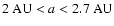 ;
and blue indicates
trans-snowline material originating from a > 2.7 AU. The top row of
charts are the results of Run Set A and the bottom charts the results of
Run Set B.
;
and blue indicates
trans-snowline material originating from a > 2.7 AU. The top row of
charts are the results of Run Set A and the bottom charts the results of
Run Set B.Open with DEXTER - 4.
- Volatile endowments. In agreement with previous models (Fogg & Nelson 2007b,a) and the work of Raymond et al. (2006) and Mandell et al. (2007), the habitable planets generated in the present model are predicted to be richly endowed with volatiles driven inward from beyond the nebular snowline by the migrating giant planet. The composition of the six habitable planet candidates, using the same crude three phases described in Fogg & Nelson (2007a), are shown as pie charts in Fig. 14 where the red sectors refer to dry material originating interior to 2 AU, the green sectors to chondritic material originating between 2 and 2.7 AU, and the blue sectors indicate the fractions originating from beyond the snowline at >2.7 AU. Even with no previous type I migration operating (Run Set A), the habitable planet candidates mentioned above have incorporated roughly a third to a half of their material from beyond the snowline. Where there has been pre-existing type I migration (Run Set B), more like three quarters of the planets' mass originates from beyond the snowline. Whether the habitable planets in question lie interior or exterior to the giant seems to make little difference to the composition. All such worlds are predicted to be richly endowed with water and gases.
4 Discussion
The key finding of the model presented in this paper, and its predecessors (Fogg & Nelson 2005,2007b,2006,2007a), that giant planets do not remove the portion of a protoplanetary disk they migrate through, or prevent subsequent terrestrial planet formation, is robust in the sense that every model variant, and independent work (Raymond et al. 2006; Mandell et al. 2007), has reproduced it. However, these models have only explored a modest region of parameter space relevant to the problem, and have inevitably adopted assumptions that simplify or omit potentially important physical processes. We have discussed a number of issues concerning parameter variations and neglected physical processes in our previous papers and restrict the discussion here to three caveats not previously considered.
- i)
- Solids disk inner boundary. The inner system
solids disk adopted here begins with its inner boundary set at
0.4 AU. Its contents are then free to evolve inward during the
maturation runs preceding the introduction of the giant at the start
of a migration scenario. By this time, in low dissipation models
(Run Set A), dynamical spreading typically results in a
modest inward movement of the disk edge to 0.3 AU (see the
upper panel of Fig. 4) so that when the giant planet
subsequently migrates down to 0.1 AU it passes through the entire
inner disk annulus. This is not necessarily the case in high
dissipation models (Run Set B) where greater inward
movement of the solids disk contents occurs during the maturation
phase (see the lower panel of Fig. 4). Thus, the
question is raised as to whether the lack of interior hot-Earths
resulting in Scenarios 1 and 2 is a realistic finding or an artifact
of the initial position of the solids disk inner boundary. What if
this boundary had been set at 0.1 AU instead? This would have
provided an additional
 of material from
which potential interior planets could have been assembled. It
cannot be ruled out therefore that some hot-Earths could grow and
survive even in early scenarios of Run Set A, especially if
the giant planet stops short of their position. However, one would
still expect them to be of lower mass and more prone to orbital
destabilization than in high dissipation models where eccentricity
damping is in play and where there has been much more extensive
prior inward migration of solids.
of material from
which potential interior planets could have been assembled. It
cannot be ruled out therefore that some hot-Earths could grow and
survive even in early scenarios of Run Set A, especially if
the giant planet stops short of their position. However, one would
still expect them to be of lower mass and more prone to orbital
destabilization than in high dissipation models where eccentricity
damping is in play and where there has been much more extensive
prior inward migration of solids.
- ii)
- Random component of initial conditions. The
solids disk with which we begin our simulations at t = 0 conforms
as a whole to a 3
 MMSN model, but is unique in the sense that
its individual particles start with randomized orbital elements.
This raises the question of how the conclusions of this paper might
depend on the seed number used to randomize these initial
conditions. We have not tested the influence of alternate seed
numbers on the particular set of simulations presented here.
However, comparison with our previous work, where different integers
have been used to seed the initial setup, shows that in scenarios
where disk maturity and dissipative forces are roughly equivalent,
the overall architectures of the post-migration systems are similar
even though details of individual planets are different. This is
because the general physical processes shown to characterise the
migration of a giant planet through an inner system disk, which lead
to the division of the original disk contents into internal and
external remnants, are largely independent of the random component
in the initial conditions and are influenced primarily by the level
and variety of dissipative forces in play - i.e. by the maturity of
the solid body swarm, the density of the gas, and whether type I
migration is active. An example of such a comparison can be seen by
referring to Fig. 12 from Fogg & Nelson (2007a), where the results of a late
scenario, matured for 1.5 Myr before the onset of giant planet
migration, in the absence of type I migration, are plotted. The
lower panel of this figure shows the evolution of this model 2 Myr
after the giant planet has stranded at 0.1 AU and its overall system
architecture is similar to its closest equivalent in the present
work: Scenario 1, shown in the top panel of Fig. 6. No
interior hot-Earth is present and protoplanets amounting to several
have been externally scattered to between 1-3 AU in both cases. The post migration evolution of this hot-Jupiter
system from Fogg & Nelson (2007a) has been run further to 30 Myr and the
results illustrated in Fogg (2008). The resemblance between that
run and the matured Scenario 1 in this paper (Fig. 10,
top panel) is even closer with a
MMSN model, but is unique in the sense that
its individual particles start with randomized orbital elements.
This raises the question of how the conclusions of this paper might
depend on the seed number used to randomize these initial
conditions. We have not tested the influence of alternate seed
numbers on the particular set of simulations presented here.
However, comparison with our previous work, where different integers
have been used to seed the initial setup, shows that in scenarios
where disk maturity and dissipative forces are roughly equivalent,
the overall architectures of the post-migration systems are similar
even though details of individual planets are different. This is
because the general physical processes shown to characterise the
migration of a giant planet through an inner system disk, which lead
to the division of the original disk contents into internal and
external remnants, are largely independent of the random component
in the initial conditions and are influenced primarily by the level
and variety of dissipative forces in play - i.e. by the maturity of
the solid body swarm, the density of the gas, and whether type I
migration is active. An example of such a comparison can be seen by
referring to Fig. 12 from Fogg & Nelson (2007a), where the results of a late
scenario, matured for 1.5 Myr before the onset of giant planet
migration, in the absence of type I migration, are plotted. The
lower panel of this figure shows the evolution of this model 2 Myr
after the giant planet has stranded at 0.1 AU and its overall system
architecture is similar to its closest equivalent in the present
work: Scenario 1, shown in the top panel of Fig. 6. No
interior hot-Earth is present and protoplanets amounting to several
have been externally scattered to between 1-3 AU in both cases. The post migration evolution of this hot-Jupiter
system from Fogg & Nelson (2007a) has been run further to 30 Myr and the
results illustrated in Fogg (2008). The resemblance between that
run and the matured Scenario 1 in this paper (Fig. 10,
top panel) is even closer with a
 planet being present in the habitable zone of both systems. We
conclude that although the specific properties of the planetary
systems which arise from our simulations depend on the exact details
of the initial setup, the general trends that we observe in our
outcomes are robust.
planet being present in the habitable zone of both systems. We
conclude that although the specific properties of the planetary
systems which arise from our simulations depend on the exact details
of the initial setup, the general trends that we observe in our
outcomes are robust.
- iii)
- Ocean planets. One effect of giant planet
migration is to drive large quantities of icy material into the
inner system, with the outcome that terrestrial planets that form in
the aftermath are predicted to be richly endowed with volatiles and
enveloped by global oceans. There is nothing about 100% ocean cover
that necessarily rules out the presence of life. Indeed, life may
have started in the Earth's oceans, and exploration beneath
ocean-covered Europa's ice shell has long been regarded as a top
priority by astrobiologists (Reynolds et al. 1987,1983). Ocean
planets in the
range however have a problem
not shared with Europa: if the depth of their oceans is 100 km, their floors are composed of high pressure phases of ice,
rather than rock, with the ice-silicate interface (and much
potentially crucial chemistry) sealed off beneath an icy mantle 100s
or 1000 s of km thick, depending on the planet's total mass and bulk
water content (Léger et al. 2004). How this would effect the solute
content of the oceans is unknown but one might speculate that some
trace elements essential for terrestrial life might be
lacking
![[*]](/icons/foot_motif.gif) .
Meteoritic infall after planetary differentiation is complete would
re-supply some rock-forming elements for dissolution into the ocean,
but solid material that deposits on the ocean floor would be denser
than the ice beneath and prone to removal by sinking into the
mantle. A related problem deepens this uncertainty. Planets
over-endowed with water might similarly possess massive atmospheres
with unexpected compositions and properties. If ocean planets are
more like thawed out versions of Titan, rather than water-rich
Earths, then habitable zone calculations that rely on models of
modest
.
Meteoritic infall after planetary differentiation is complete would
re-supply some rock-forming elements for dissolution into the ocean,
but solid material that deposits on the ocean floor would be denser
than the ice beneath and prone to removal by sinking into the
mantle. A related problem deepens this uncertainty. Planets
over-endowed with water might similarly possess massive atmospheres
with unexpected compositions and properties. If ocean planets are
more like thawed out versions of Titan, rather than water-rich
Earths, then habitable zone calculations that rely on models of
modest
 atmospheres, coupled to a
carbonate-silicate cycle and continental weathering
(e.g. Selsis et al. 2007; Kasting et al. 1993; von Bloh et al. 2007), may not be relevant.
atmospheres, coupled to a
carbonate-silicate cycle and continental weathering
(e.g. Selsis et al. 2007; Kasting et al. 1993; von Bloh et al. 2007), may not be relevant.
5 Conclusions
All previous published models of terrestrial planet formation in the presence of type II giant planet migration have neglected the issue of what causes the giant planet to come to rest in its final orbit and have simply switched off migration forces at a pre-defined distance from the central star (Fogg & Nelson 2005; Raymond et al. 2006; Fogg & Nelson 2007b; Mandell et al. 2007; Fogg & Nelson 2007a). This latest model is the first simulation of this type to include a self-consistent scenario for the stranding of the giant planet, which comes to rest naturally at the point when the gaseous fraction of the protoplanetary disk is lost via a combination of accretion onto the central star and photoevaporation.
The results of the earliest scenarios - those which simulate
hot-Jupiter emplacement at
![]() AU - are very
similar to the late scenarios of Fogg & Nelson (2007b,a), where the
evolution of the nebula is advanced and dissipative forces that stem
from the presence of gas are relatively weak. Most of the inner
system disk solids survive the traverse of the giant planet and most
of this surviving matter is scattered into higher orbits where
planet formation can resume. Water-rich habitable planets are
possible within a habitable zone that is far removed from the final
position of the giant planet. Where dissipative processes are
enhanced by type I migration, one or two hot-Earths or hot-Neptunes
are found to persist in orbits interior to the giant planet.
AU - are very
similar to the late scenarios of Fogg & Nelson (2007b,a), where the
evolution of the nebula is advanced and dissipative forces that stem
from the presence of gas are relatively weak. Most of the inner
system disk solids survive the traverse of the giant planet and most
of this surviving matter is scattered into higher orbits where
planet formation can resume. Water-rich habitable planets are
possible within a habitable zone that is far removed from the final
position of the giant planet. Where dissipative processes are
enhanced by type I migration, one or two hot-Earths or hot-Neptunes
are found to persist in orbits interior to the giant planet.
In ``warm-Jupiter'' type scenarios, where
![]() AU,
the bulk of the disk solids survive as before, but more complex
systems of hot terrestrial planets interior to the giant are
predicted, in larger numbers with increasing
AU,
the bulk of the disk solids survive as before, but more complex
systems of hot terrestrial planets interior to the giant are
predicted, in larger numbers with increasing ![]() .
If
strong type I migration forces are a genuine influence on planet
formation, relatively crowded systems of interior planets are
predicted, although it has not been practical to check this forecast
with Gyr-long integrations. Habitable planets in low eccentricity
warm-Jupiter systems appear possible if the giant planet makes a
limited incursion into the outer regions of the habitable zone, or
traverses its entire width and keeps going until it ceases migrating
at a radial distance of less than half that of the HZ's inner edge:
i.e. the giant planet's final orbit lies outside the region of
.
If
strong type I migration forces are a genuine influence on planet
formation, relatively crowded systems of interior planets are
predicted, although it has not been practical to check this forecast
with Gyr-long integrations. Habitable planets in low eccentricity
warm-Jupiter systems appear possible if the giant planet makes a
limited incursion into the outer regions of the habitable zone, or
traverses its entire width and keeps going until it ceases migrating
at a radial distance of less than half that of the HZ's inner edge:
i.e. the giant planet's final orbit lies outside the region of ![]() 0.3-1.5 AU for a 1
0.3-1.5 AU for a 1 ![]() star. If giant planets
strand within this region, the presence of habitable planets remains
a possibility if they are located in a stable 1:1 resonance with the
giant. These findings should hold for stars with different
luminosities with an appropriate scaling of radial distance.
star. If giant planets
strand within this region, the presence of habitable planets remains
a possibility if they are located in a stable 1:1 resonance with the
giant. These findings should hold for stars with different
luminosities with an appropriate scaling of radial distance.
![\begin{figure}
\par\includegraphics[width=7cm,clip]{figures_recadrées/11305fig15.eps}
\end{figure}](/articles/aa/full_html/2009/17/aa11305-08/img135.gif) |
Figure 15:
Data of low eccentricity exoplanets
using data from the Extrasolar Planets
Encyclopedia: http://exoplanet.eu. Plotted objects correspond to
the type of warm-Jupiters within the remit of the model presented here: solitary giant planets
orbiting single stars with
|
| Open with DEXTER | |
However, warm-Jupiter type exoplanets with near-circular orbits,
i.e.
![]() ,
are relatively uncommon and e is typically
observed to be considerably higher. Many of these exoplanets may
have had an origin involving mutual giant planet scattering, perhaps
combined with migration (e.g. Moorhead & Adams 2005; Ford et al. 2001; Papaloizou & Terquem 2001),
as opposed to the strongly damped pure type II migration mechanism
adopted here. Nevertheless, low-e and solitary warm-Jupiters are
known, which presumably could have originated in a similar manner to
that simulated here. Figure 15 uses data from the
Extrasolar Planets Encyclopedia to plot exoplanetary data between
a
= 0.1-1.8 AU vs.
e = 0-0.05 which might be regarded as lying
within the remit of the model. Solitary giant planets around single
stars are plotted and labelled with their names. Four of these
exoplanets,
,
are relatively uncommon and e is typically
observed to be considerably higher. Many of these exoplanets may
have had an origin involving mutual giant planet scattering, perhaps
combined with migration (e.g. Moorhead & Adams 2005; Ford et al. 2001; Papaloizou & Terquem 2001),
as opposed to the strongly damped pure type II migration mechanism
adopted here. Nevertheless, low-e and solitary warm-Jupiters are
known, which presumably could have originated in a similar manner to
that simulated here. Figure 15 uses data from the
Extrasolar Planets Encyclopedia to plot exoplanetary data between
a
= 0.1-1.8 AU vs.
e = 0-0.05 which might be regarded as lying
within the remit of the model. Solitary giant planets around single
stars are plotted and labelled with their names. Four of these
exoplanets,
![]() ,
HD 27894 b, HD 192263 b and
HD 4208 b occur in systems where there is dynamical room for
terrestrial planets in the habitable zone according to the stability
calculations of Jones et al. (2005,2006). Systems containing the
exoplanets HD 224693 b (Jones et al. 2006), HD 104985 b and HD 59686 b
(Jones et al. 2005) could also have hosted planets in their habitable
zones in the past before their primaries left the main sequence.
According to the results of the model presented in this paper, it
appears feasible that habitable planets could have originated in
these systems as well.
,
HD 27894 b, HD 192263 b and
HD 4208 b occur in systems where there is dynamical room for
terrestrial planets in the habitable zone according to the stability
calculations of Jones et al. (2005,2006). Systems containing the
exoplanets HD 224693 b (Jones et al. 2006), HD 104985 b and HD 59686 b
(Jones et al. 2005) could also have hosted planets in their habitable
zones in the past before their primaries left the main sequence.
According to the results of the model presented in this paper, it
appears feasible that habitable planets could have originated in
these systems as well.
References
- Adams, F. C., & Laughlin, G. 2003, Icarus, 163, 290 [NASA ADS] [CrossRef]
- Alexander, R. D., Clarke, C. J., & Pringle, J. E. 2006, MNRAS, 369, 229 [NASA ADS] [CrossRef]
- Armitage, P. J. 2003, ApJ, 582, L47 [NASA ADS] [CrossRef] (In the text)
- Armitage, P. J. 2007, ApJ, 665, 1381 [NASA ADS] [CrossRef]
- Armitage, P. J., Livio, M., Lubow, S. H., & Pringle, J. E. 2002, MNRAS, 334, 248 [NASA ADS] [CrossRef]
- Asphaug, E., Agnor, C., & Williams, Q. 2006, Nature, 439, 155 [NASA ADS] [CrossRef]
- Bertout, C. 1989, ARA&A, 27, 351 [NASA ADS] [CrossRef] (In the text)
- Boss, A. P. 2000, ApJ, 536, L101 [NASA ADS] [CrossRef]
- Butler, P., Wright, J. T., Marcy, G. W., et al. 2006, ApJ, 646, 505 [NASA ADS] [CrossRef] (In the text)
- Canup, R. M., & Pierazzo, E. 2006, LPI, 37, 2146 [NASA ADS]
- Chambers, J. E. 1999, MNRAS, 304, 793 [NASA ADS] [CrossRef] (In the text)
- Clarke, C. J., Gendrin, A., & Sotomayor, M. 2001, MNRAS, 328, 485 [NASA ADS] [CrossRef]
- Cresswell, P., & Nelson, R. P. 2006, A&A, 450, 833 [NASA ADS] [CrossRef] [EDP Sciences]
- Cresswell, P., & Nelson, R. P. 2008, A&A, 482, 677 [NASA ADS] [CrossRef] [EDP Sciences]
- Daisaka, J. K., Tanaka, H., & Ida, S. 2006, Icarus, 185, 492 [NASA ADS] [CrossRef]
- Dvorak, R., Pilat-Lohinger, E., Schwarz, R., & Freistetter, F. 2004, A&A, 426, L37 [NASA ADS] [CrossRef] [EDP Sciences] (In the text)
- Erdi, B., & Sandor, Z. 2004, CeMDA, 92, 113 [NASA ADS] [CrossRef] (In the text)
- Fogg, M. J. 2008, Terrestrial planet formation in exoplanetary systems, Ph.D. Thesis (University of London), 103 (In the text)
- Fogg, M. J., & Nelson, R. P. 2005, A&A, 441, 791 [NASA ADS] [CrossRef] [EDP Sciences]
- Fogg, M. J., & Nelson, R. P. 2006, Intnl. J. Astrobiol., 5, 199 [CrossRef]
- Fogg, M. J., & Nelson, R. P. 2007a, A&A, 461, 1195 [NASA ADS] [CrossRef] [EDP Sciences]
- Fogg, M. J., & Nelson, R. P. 2007b, A&A, 472, 1003 [NASA ADS] [CrossRef] [EDP Sciences]
- Ford, E. B., Havlickova, M., & Rasio, F. A. 2001, Icarus, 150, 303 [NASA ADS] [CrossRef]
- Genda, H., & Abe, Y. 2005, Nature, 433, 842 [NASA ADS] [CrossRef]
- Goldreich, P., & Sari, R. 2003, ApJ, 585, 1024 [NASA ADS] [CrossRef]
- Goldreich, P., Lithwick, Y., & Sari, R. 2004, ApJ, 614, 497 [NASA ADS] [CrossRef] (In the text)
- Haisch, K. E., Lada, E. A., & Lada, C. J. 2001, ApJ, 553, L153 [NASA ADS] [CrossRef] (In the text)
- Hayashi, C. 1981, Prog. Theor. Phys. Suppl., 70, 35 [NASA ADS] [CrossRef] (In the text)
- Hollenbach, D., Johnstone, D., Lizano, S., & Shu, F. 1994, ApJ, 428, 654 [NASA ADS] [CrossRef] (In the text)
- Jones, B. W., Underwood, D. R., & Sleep, P. N. 2005, ApJ, 622, 1091 [NASA ADS] [CrossRef]
- Jones, B. W., Sleep, P. N., & Underwood, D. R. 2006, Intnl. J. Astrobiol., 5, 251 [CrossRef]
- Kasting, J. F., Whitmire, D. P., & Reynolds, R. T. 1993, Icarus, 101, 108 [NASA ADS] [CrossRef] (In the text)
- Kokubo, E., & Ida, S. 2000, Icarus 143, 15 (In the text)
- Kuchner, M. J., & Lecar, M. 2002, ApJ, 574, L87 [NASA ADS] [CrossRef]
- Léger, A., Selsis, F., Sotin, C., et al. 2004, Icarus, 169, 499 [NASA ADS] [CrossRef] (In the text)
- Lin, D. N. C., & Ida, S. 1997, ApJ, 477, 781 [NASA ADS] [CrossRef]
- Lin, D. N. C., & Papaloizou, J. C. B. 1986, ApJ, 309, 846 [NASA ADS] [CrossRef]
- Lin, D. N. C., Bodenheimer, P., & Richardson, D. C. 1996, Nature, 380, 606 [NASA ADS] [CrossRef]
- Lineweaver, C. H. 2001, Icarus, 151, 307 [NASA ADS] [CrossRef]
- Lineweaver, C. H., Fenner, Y., & Gibson, B. K. 2004, Science, 303, 59 [NASA ADS] [CrossRef]
- Lissauer, J. J. 1987, Icarus, 69, 249 [NASA ADS] [CrossRef]
- Mandell, A. M., Raymond, S. N., & Sigurdsson, S. 2007, ApJ, 660, 823 [NASA ADS] [CrossRef]
- Marzari, F., & Weidenschilling, S. J. 2002, Icarus, 156, 570 [NASA ADS] [CrossRef]
- Masset, F. S., Morbidelli, A., Crida, A., & Ferreira, J. 2006, ApJ, 642, 478 [NASA ADS] [CrossRef]
- McArthur, B. E., Endl, M., Cochran, G., et al. 2004, ApJ, 614, L81 [NASA ADS] [CrossRef] (In the text)
- McNeil, D., Duncan, M., & Levison, H. F. 2005, AJ, 130, 2884 [NASA ADS] [CrossRef]
- Moorhead, A. V., & Adams, F. C. 2005, Icarus, 178, 517 [NASA ADS] [CrossRef]
- Moorhead, A. V., & Adams, F. C. 2008, Icarus, 193, 475 [NASA ADS] [CrossRef]
- Nelson, R. P., Papaloizou, J. C. B., Masset, F. S., & Kley, W. 2000, MNRAS, 318, 18 [NASA ADS] [CrossRef]
- Ogilvie, G. I., & Lubow, S. H. 2003, ApJ, 587, 398 [NASA ADS] [CrossRef]
- Papaloizou, J. C. B. 2007, A&A, 463, 775 [NASA ADS] [CrossRef] [EDP Sciences]
- Papaloizou, J. C. B., & Larwood, J. D. 2000, MNRAS, 315, 823 [NASA ADS] [CrossRef]
- Papaloizou, J. C. B., & Nelson, R. P. 2005, A&A, 433, 247 [NASA ADS] [CrossRef] [EDP Sciences]
- Papaloizou, J. C. B., & Terquem, C. 2001, MNRAS, 325, 221 [NASA ADS] [CrossRef]
- Papaloizou, J. C. B., Nelson, R. P., & Masset, F. 2001, A&A, 366, 263 [NASA ADS] [CrossRef] [EDP Sciences]
- Pollack, J. B., Hubickyj, O., Bodenheimer, P., et al. 1996, Icarus, 124, 62 [NASA ADS] [CrossRef]
- Raymond, S. N., Quinn, T., & Lunine, J. I. 2004, Icarus, 168, 1 [NASA ADS] [CrossRef]
- Raymond, S. N., Mandell, A. M., & Sigurdsson, S. 2006, Science, 313, 1413 [NASA ADS] [CrossRef]
- Raymond, S. N., Quinn, T., & Lunine, J. I. 2007, AsBio, 7, 66 [NASA ADS]
- Raymond, S. N., Barnes, R., Armitage, P. J., & Gorelick, N. 2008, ApJ, 687, L107 [NASA ADS] [CrossRef] (In the text)
- Reynolds, R. T., Squyres, S. W., Colburn, D. S., & McKay, C. P. 1983, Icarus, 56, 246 [NASA ADS] [CrossRef]
- Reynolds, R. T., McKay, C. P., & Kasting, J. F. 1987, AdSpR, 7, 125 [NASA ADS]
- Selsis, F., Kasting, J. F., Levrard, B., et al. 2007, A&A, 476, 1373 [NASA ADS] [CrossRef] [EDP Sciences]
- Simon, M., & Prato, L. 1995, ApJ, 450, 824 [NASA ADS] [CrossRef]
- Takeuchi, T., Miyama, S. N., & Lin, D. N. C. 1996, ApJ, 460, 832 [NASA ADS] [CrossRef]
- Tanaka, H., & Ward, W. R. 2004, ApJ, 602, 388 [NASA ADS] [CrossRef]
- Tanaka, H., Takeuchi, T., & Ward, W. R. 2002, ApJ, 565, 1257 [NASA ADS] [CrossRef]
- Thommes, E. W., Duncan, M. J., & Levison, H. F. 2003, Icarus, 161, 431 [NASA ADS] [CrossRef] (In the text)
- Trilling, D. E., Benz, W., Guillot, T., et al. 1998, ApJ, 500, 428 [NASA ADS] [CrossRef] (In the text)
- von Bloh, W., Bounama, C., Cuntz, M., & Franck, S. 2007, A&A, 476, 1365 [NASA ADS] [CrossRef] [EDP Sciences]
- Ward, P. D., & Brownlee, D. 2000, Rare Earth: Why complex life is uncommon in the universe (New York: Copernicus Books) (In the text)
- Ward, W. R. 1997, Icarus, 126, 261 [NASA ADS] [CrossRef]
- Wolk, S. J., & Walter, F. M. 1996, AJ, 111, 2066 [NASA ADS] [CrossRef]
Footnotes
- ...
 Myr
Myr
- Note that the gap between the t = 1.82 and 1.83 Myr curves is because of the substantial depletion of disk gas at these late times, dictating the removal of the quantity required for the giant planet's envelope from a wider annulus of the disk than previously.
- ... points
- The phrase ``end point'' here refers to the time at which type II migration of the giant planet ceases due to gas disk dispersal.
- ...
lacking
- The elemental requirements of non-terrestrial life are another matter and unknown.
All Tables
Table 1: Data describing initial solids disk set-up.
Table 2: Matured solids disk at the start of the stranding window.
All Figures
| |
Figure 1:
Upper panel: mass of the nebular gas vs. time: the blue curve
represents our former model where mass loss occurs solely via
viscous accretion onto the central star; the red curve
represents our new model including photoevaporation. Lower panel:
accretion rate onto the central star
|
| Open with DEXTER | |
| In the text | |
| |
Figure 2: Model gas disk surface density evolution. The uppermost curve is the initial condition; successive curves are labeled with their age in Myr. |
| Open with DEXTER | |
| In the text | |
| |
Figure 3:
Migration and stranding of 0.5 MJ giant planets
in our present and previous models. Giant planet semi major axis in
AU is plotted against |
| Open with DEXTER | |
| In the text | |
| |
Figure 4: Eccentricity vs. semi-major axis for matured solids disks at 1.77 Myr for no type I migration ( top panel) and with type I migration ( bottom panel). Grey dots are super-planetesimals; red and blue circles are protoplanets originating interior and exterior to the snowline respectively. Gas densities are read on the right hand axes: the upper blue lines show gas density at t = 0 and the lower cyan lines are the current densities. |
| Open with DEXTER | |
| In the text | |
| |
Figure 5: Total solids mass in 0.5 AU width bins at t = 1.77 Myr for maturation runs with no type I migration (magenta bars) and with type I migration (cyan bars). |
| Open with DEXTER | |
| In the text | |
| |
Figure 6:
Run Set A. End points of scenarios that exclude type I
migration, when the giant planet strands at its
final semi-major axis. Eccentricity is plotted vs. semi-major
axis with symbols colour coded as in Fig. 4 and
sized according to the mass key. Scenario ID is given at the
top left of each panel. Protoplanets interior to the giant, or
within 1-2 AU, are labelled with their mass in
|
| Open with DEXTER | |
| In the text | |
| |
Figure 7:
Run Set B. End points of scenarios that include type I
migration, when the giant planet strands at its
final semi-major axis. Eccentricity is plotted vs. semi-major
axis with symbols colour coded as in Fig. 4 and
sized according to the mass key. Scenario ID is given at the
top left of each panel. Protoplanets interior to the giant, or
within 1-2 AU, are labelled with their mass in
|
| Open with DEXTER | |
| In the text | |
| |
Figure 8: Fate of the disk mass at the end points of Run Set A and B. Data include the cumulative % of initial solids disk in the shepherded or scattered remnant, or lost from the disk. |
| Open with DEXTER | |
| In the text | |
| |
Figure 9:
Protoplanet mass fraction
|
| Open with DEXTER | |
| In the text | |
| |
Figure 10:
Run Set A. Gas-free accretion results of scenarios
that exclude previous type I migration. Eccentricity is plotted vs. semi-major
axis with symbols colour coded as in previous examples and
sized according to the mass key. Scenario ID is given at the
top left of each panel. System age is given at the top right of each panel.
Protoplanets interior to the giant, or within 1-2 AU, are labelled with their
mass in
|
| Open with DEXTER | |
| In the text | |
| |
Figure 11:
Run Set B. Gas-free accretion results of scenarios that include previous type I
migration. Scenario ID is given at the top left of each panel. System age is given at the top right of each
panel. Protoplanets interior to the giant, or within 1-2 AU, are
labelled with their mass in
|
| Open with DEXTER | |
| In the text | |
![\begin{figure}
\par\includegraphics[width=7.5cm,clip]{figures_recadrées/11305fig12.eps}
\end{figure}](/articles/aa/full_html/2009/17/aa11305-08/img121.gif) |
Figure 12:
Destabilization of the resonant convoy in Scenario |
| Open with DEXTER | |
| In the text | |
| |
Figure 13:
Inner systems of Scenarios |
| Open with DEXTER | |
| In the text | |
![\begin{figure}
\par\includegraphics[width=6cm,clip]{11305fig14.eps}
\end{figure}](/articles/aa/full_html/2009/17/aa11305-08/img126.gif) |
Figure 14:
Material composition of habitable planet candidates from our
simulations. Red
indicates material of provenance a < 2 AU; green indicates material of
provenance
|
| Open with DEXTER | |
| In the text | |
| |
Figure 15:
Data of low eccentricity exoplanets
using data from the Extrasolar Planets
Encyclopedia: http://exoplanet.eu. Plotted objects correspond to
the type of warm-Jupiters within the remit of the model presented here: solitary giant planets
orbiting single stars with
|
| Open with DEXTER | |
| In the text | |
Copyright ESO 2009
Current usage metrics show cumulative count of Article Views (full-text article views including HTML views, PDF and ePub downloads, according to the available data) and Abstracts Views on Vision4Press platform.
Data correspond to usage on the plateform after 2015. The current usage metrics is available 48-96 hours after online publication and is updated daily on week days.
Initial download of the metrics may take a while.