| Issue |
A&A
Volume 497, Number 3, April III 2009
|
|
|---|---|---|
| Page(s) | 991 - 1007 | |
| Section | Numerical methods and codes | |
| DOI | https://doi.org/10.1051/0004-6361/200810824 | |
| Published online | 09 February 2009 | |
A Markov Chain Monte Carlo technique to sample transport and source parameters of Galactic cosmic rays
I. Method and results for the Leaky-Box model
A. Putze1 - L. Derome1 - D. Maurin2 - L. Perotto1,3 - R. Taillet4,5
1 - Laboratoire de Physique Subatomique et de
Cosmologie LPSC, 53 avenue des Martyrs,
38026 Grenoble, France
2 - Laboratoire de Physique Nucléaire et des Hautes
Énergies LPNHE, Tour 33, Jussieu,
75005 Paris, France
3 - Laboratoire de l'accélérateur linéaire LAL,
Université Paris-Sud 11, Bâtiment 200, BP 34, 91898 Orsay Cedex, France
4 - Laboratoire de Physique Théorique LAPTH, Chemin de Bellevue BP 110,
7494i1 Annecy-le-Vieux, France
5 -
Université de Savoie, 73011 Chambéry, France
Received 18 August 2008 / Accepted 7 December 2008
Abstract
Context. Propagation of charged cosmic-rays in the Galaxy depends on the transport parameters, whose number can be large depending on the propagation model under scrutiny. A standard approach for determining these parameters is a manual scan, leading to an inefficient and incomplete coverage of the parameter space.
Aims. In analyzing the data from forthcoming experiments, a more sophisticated strategy is required. An automated statistical tool is used, which enables a full coverage of the parameter space and provides a sound determination of the transport and source parameters. The uncertainties in these parameters are also derived.
Methods. We implement a Markov Chain Monte Carlo (MCMC), which is well suited to multi-parameter determination. Its specificities (burn-in length, acceptance, and correlation length) are discussed in the context of cosmic-ray physics. Its capabilities and performances are explored in the phenomenologically well-understood Leaky-Box Model.
Results. From a technical point of view, a trial function based on binary-space partitioning is found to be extremely efficient, allowing a simultaneous determination of up to nine parameters, including transport and source parameters, such as slope and abundances. Our best-fit model includes both a low energy cut-off and reacceleration, whose values are consistent with those found in diffusion models. A Kolmogorov spectrum for the diffusion slope (
 )
is excluded. The marginalised probability-density function for
)
is excluded. The marginalised probability-density function for  and
and  (the slope of the source spectra) are
 and
and
 ,
depending on the dataset used and the number of free parameters in the fit. All source-spectrum parameters (slope and abundances) are positively correlated among themselves and with the reacceleration strength, but are negatively correlated with the other propagation parameters.
,
depending on the dataset used and the number of free parameters in the fit. All source-spectrum parameters (slope and abundances) are positively correlated among themselves and with the reacceleration strength, but are negatively correlated with the other propagation parameters.
Conclusions. The MCMC is a practical and powerful tool for cosmic-ray physic analyses. It can be used to confirm hypotheses concerning source spectra (e.g., whether
 )
and/or determine whether different datasets are compatible. A forthcoming study will extend our analysis to more physical diffusion models.
)
and/or determine whether different datasets are compatible. A forthcoming study will extend our analysis to more physical diffusion models.
Key words: diffusion - methods: statistical - ISM: cosmic rays
1 Introduction
One issue of cosmic-ray (CR) physics is the determination of the transport
parameters in the Galaxy. This determination is based on the analysis
of the secondary-to-primary ratio (e.g., B/C, sub-Fe/Fe), for which
the dependence on the source spectra is negligible, and the ratio remains
instead mainly sensitive to the propagation processes (e.g., Maurin et al. 2001,
and references therein).
For almost 20 years, the determination of these parameters relied
mostly on the most constraining data, namely the HEAO-3 data, taken
in 1979, which covered the  1-35 GeV/n range (Engelmann et al. 1990).
For the first time since HEAO-3, several satellite
or balloon-borne experiments (see ICRC 2007 reporter's
talk Blasi 2008) have acquired higher quality
data in the same energy range or covered a
scarcely explored range (in terms of energy, 1 TeV/n-PeV/n,
or in terms of nucleus): from the balloon-borne side, the ATIC collaboration has presented
the B/C ratio at 0.5-50 GeV/n (Panov et al. 2007), and for H to Fe fluxes at 100 GeV-100 TeV
(Panov et al. 2006). At higher energy, two long-duration balloon flights
will soon provide spectra for Z=1-30 nuclei. The TRACER collaboration has
published spectra for oxygen up to iron in the GeV/n-TeV/n
range (Ave et al. 2008; Boyle et al. 2007). A second long-duration flight took
place in summer 2006, during which the instrument was designed to have a wider dynamic-range
capability and to measure lighter B, C, and N elements. The CREAM experiment (Seo et al. 2004)
flew a cumulative duration of 70 days in December 2004 and December 2005
(Seo et al. 2006, and preliminary results in
Marrocchesi et al. 2006; and Wakely et al. 2006), and again
in December 2007. A fourth flight was scheduled for
December 2008![]() .
Exciting data will arrive from the PAMELA satellite
(Picozza et al. 2007), which was successfully launched in June
2006 (Casolino et al. 2008).
.
Exciting data will arrive from the PAMELA satellite
(Picozza et al. 2007), which was successfully launched in June
2006 (Casolino et al. 2008).
With this wealth of new data, it is relevant to question the method used to extract
the propagation parameters. The value of these parameters is important to many theoretical
and astrophysical questions, because they are linked, amongst others, to the transport
in turbulent magnetic fields,
sources of CRs, and  -ray diffuse emission (see Strong et al. 2007,
for a recent review and references). It also proves to be crucial for indirect
dark-matter detection studies (e.g., Donato et al. 2004; Delahaye et al. 2008).
The usage in the past has been based mostly on a manual or
semi-automated - hence partial - coverage of the parameter space (e.g.,
Webber et al. 1992; Strong & Moskalenko 1998; Jones et al. 2001).
More complete scans were performed in Maurin et al. (2001,2002), and Lionetto et al. (2005), although in an inefficient
manner: the addition of a single new free parameter (as completed for example
in Maurin et al. 2002; compared to Maurin et al. 2001)
remains prohibitive in terms of computing time.
To remedy these shortcomings, we propose to use the Markov Chain Monte Carlo
(MCMC) algorithm, which is widely used in cosmological parameter estimates
(e.g., Christensen et al. 2001; Lewis & Bridle 2002; and
Dunkley et al. 2005). One goal of the paper is to confirm whether
the MCMC algorithm can provide similar benefits in CR physics.
-ray diffuse emission (see Strong et al. 2007,
for a recent review and references). It also proves to be crucial for indirect
dark-matter detection studies (e.g., Donato et al. 2004; Delahaye et al. 2008).
The usage in the past has been based mostly on a manual or
semi-automated - hence partial - coverage of the parameter space (e.g.,
Webber et al. 1992; Strong & Moskalenko 1998; Jones et al. 2001).
More complete scans were performed in Maurin et al. (2001,2002), and Lionetto et al. (2005), although in an inefficient
manner: the addition of a single new free parameter (as completed for example
in Maurin et al. 2002; compared to Maurin et al. 2001)
remains prohibitive in terms of computing time.
To remedy these shortcomings, we propose to use the Markov Chain Monte Carlo
(MCMC) algorithm, which is widely used in cosmological parameter estimates
(e.g., Christensen et al. 2001; Lewis & Bridle 2002; and
Dunkley et al. 2005). One goal of the paper is to confirm whether
the MCMC algorithm can provide similar benefits in CR physics.
The analysis is performed in the framework of the Leaky-Box Model (LBM), a simple and widely used propagation model. This model contains most of the CR phenomenology and is well adapted to a first implementation of the MCMC tool. In Sect. 2, we highlight the appropriateness of the MCMC compared to other algorithms used in the field. In Sect. 3, the MCMC algorithm is presented. In Sect. 4, this algorithm is implemented in the LBM. In Sect. 5, we discuss the MCMC advantages and effectiveness in the field of CR physics, and present results for the LBM. We present our conclusions in Sect. 6. Application of the MCMC technique to a more up-to-date modelling, such as diffusion models, is left to a forthcoming paper.
2 Link between the MCMC, the CR data, and the model parameters
Various models describe the propagation of CRs in the interstellar medium (Evoli et al. 2008; Berezhko et al. 2003; Maurin et al. 2001; Strong & Moskalenko 1998; Shibata et al. 2006; Webber et al. 1992; Bloemen et al. 1993). Each model is based on his own specific geometry and has its own set of parameters, characterising the Galaxy properties. The MCMC approach aims to study quantitatively how the existing (or future) CR measurements can constrain these models or, equivalently, how in such models the set of parameters (and their uncertainties) can be inferred from the data.
In practice, a given set of parameters in a propagation model implies, e.g.,
a given B/C ratio. The model parameters are constrained such as
to reproduce the measured ratio. The standard practice used to
be an eye inspection of the goodness of fit to the data. This
was replaced by the  analysis in recent papers:
assuming the
statistics is applicable to the problem at stake,
confidence intervals in these parameters can be extracted
(see Appendix A).
analysis in recent papers:
assuming the
statistics is applicable to the problem at stake,
confidence intervals in these parameters can be extracted
(see Appendix A).
The main drawback of this approach is the computing time required
to extend the calculation of the
surface to a wider parameter
space. This is known as the curse of dimensionality, due to the
exponential increase in volume associated with adding extra dimensions
to the parameter space, while the good regions of this space
(for instance where the model fits the data) only fill a tiny volume.
This is where the MCMC approach, based on the Bayesian statistics,
is superior to a grid approach. As in the grid approach, one end-product
of the analysis is the surface, but with a more efficient sampling
of the region of interest.
Moreover, as opposed to classical statistics, which is based
on the construction of estimators of the parameters, Bayesian statistics
assumes the unknown parameters to be random variables. As such, their
full distribution - the so-called conditional probability-density function (PDF) - given
some experimental data (and some prior density for these parameters, see below)
can be generated.
To summarise, the MCMC algorithm provides the PDF of the model parameters, based on selected experimental data (e.g., B/C). The mean value and uncertainty in these parameters are by-products of the PDF. The MCMC enables the enlargement of the parameter space at a minimal computing time cost (although the MCMC and Metropolis-Hastings algorithms used here are not the most efficient one). The technicalities of the MCMC are briefly described below. The reader is referred to Neal (1993) and MacKay (2003) for a more substantial coverage of the subject.
3 Markov Chain Monte Carlo (MCMC)
Considering a model depending on m parameters
we aim to determine the conditional PDF of the parameters given the data,
 .
This so-called
posterior probability quantifies the change in the degree of belief one
can have in the m parameters of the model in the light of the data.
Applied to the parameter inference, Bayes theorem is
.
This so-called
posterior probability quantifies the change in the degree of belief one
can have in the m parameters of the model in the light of the data.
Applied to the parameter inference, Bayes theorem is
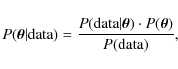
where
 is the data probability (the latter does not depend on the
parameters and hence, can be considered to be a normalisation factor).
This theorem links the posterior probability to the
likelihood of the data
is the data probability (the latter does not depend on the
parameters and hence, can be considered to be a normalisation factor).
This theorem links the posterior probability to the
likelihood of the data
 and the so-called prior probability,
 ,
indicating the degree
of belief one has before observing the data.
To extract information about a single parameter,
,
indicating the degree
of belief one has before observing the data.
To extract information about a single parameter,
 ,
the posterior density is integrated over all other parameters
,
the posterior density is integrated over all other parameters
 in a procedure called marginalisation. Finally,
by integrating the individual posterior PDF further, we are able to determine
the expectation value, confidence level, or higher order mode of the parameter
.
This illustrates the technical difficulty of Bayesian parameter estimates:
determining the individual posterior PDF requires a high-dimensional
integration of the overall posterior density. Thus, an efficient sampling
method for the posterior PDF is mandatory.
For models of more than a few parameters, regular grid-sampling approaches
are not applicable and statistical techniques are required (Cowan 1997).
in a procedure called marginalisation. Finally,
by integrating the individual posterior PDF further, we are able to determine
the expectation value, confidence level, or higher order mode of the parameter
.
This illustrates the technical difficulty of Bayesian parameter estimates:
determining the individual posterior PDF requires a high-dimensional
integration of the overall posterior density. Thus, an efficient sampling
method for the posterior PDF is mandatory.
For models of more than a few parameters, regular grid-sampling approaches
are not applicable and statistical techniques are required (Cowan 1997).
Among these techniques, MCMC algorithms have been fully tried and
tested for Bayesian parameter inference (Neal 1993; MacKay 2003).
MCMC methods explore any target distribution given by a vector of
parameters
 ,
by generating a sequence of n points (hereafter a
chain)
,
by generating a sequence of n points (hereafter a
chain)
| (3) |
Each
 is a vector of m components (as defined in
Eq. (1)). In addition, the chain is Markovian in the sense that
the distribution of
is a vector of m components (as defined in
Eq. (1)). In addition, the chain is Markovian in the sense that
the distribution of
 is influenced entirely
by the value of
is influenced entirely
by the value of
 .
MCMC algorithms are developed so that the time
spent by the Markov chain in a region of the parameter space is proportional to
the target PDF value in this region. Hence, from
such a chain, one can obtain an independent sampling of the PDF.
The target PDF as well as all marginalised PDF are estimated by counting the
number of samples within the related region of parameter space.
.
MCMC algorithms are developed so that the time
spent by the Markov chain in a region of the parameter space is proportional to
the target PDF value in this region. Hence, from
such a chain, one can obtain an independent sampling of the PDF.
The target PDF as well as all marginalised PDF are estimated by counting the
number of samples within the related region of parameter space.
Below, we provide a brief introduction to an MCMC using the Metropolis-Hastings algorithm (see Neal 1993; MacKay 2003, Chap. 29, for further details and references).
3.1 The algorithm
The prescription that we use to generate the Markov chains from the unknown target
distribution is the so-called Metropolis-Hastings algorithm. The Markov chain increases by
jumping from the current point in the parameter space
to the following
 .
As said before, the PDF of the new point only depends on the
current point, i.e.
.
As said before, the PDF of the new point only depends on the
current point, i.e.
![]() .
This quantity defines the transition
probability for state
from the state
.
The Metropolis-Hastings algorithm specifies
.
This quantity defines the transition
probability for state
from the state
.
The Metropolis-Hastings algorithm specifies
 to ensure that the stationary distribution of the chain asymptotically
tends to the target PDF one wishes to sample from.
to ensure that the stationary distribution of the chain asymptotically
tends to the target PDF one wishes to sample from.
At each step i (corresponding to a
state
), a trial state
 is
generated from a proposal density
is
generated from a proposal density
 .
This proposal density is chosen so that samples can be easily generated
(e.g., a Gaussian distribution centred on the current state).
The state
is accepted or rejected depending on
the following criterion. By forming the quantity
.
This proposal density is chosen so that samples can be easily generated
(e.g., a Gaussian distribution centred on the current state).
The state
is accepted or rejected depending on
the following criterion. By forming the quantity
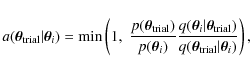
the trial state is accepted as a new state with a probability a (rejected with probability 1-a). The transition probability is then
If accepted,
 ,
whereas if rejected,
the new state is equivalent to the current state,
,
whereas if rejected,
the new state is equivalent to the current state,
 .
This criterion ensures that once at its equilibrium, the chain samples the target
distribution
.
If the proposal density
is chosen to be symmetric, it cancels out in the expression of the acceptance probability,
which becomes:
.
This criterion ensures that once at its equilibrium, the chain samples the target
distribution
.
If the proposal density
is chosen to be symmetric, it cancels out in the expression of the acceptance probability,
which becomes:
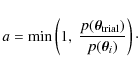
We note that the process requires only evaluations of ratios of the target PDF. This is a major virtue of this algorithm, in particular for Bayesian applications, in which the normalisation factor in Eq. (2),
3.2 Chain analysis
The chain analysis refers to the study of several properties of the chains. The following quantities are inspected in order to convert the chains in PDFs.
Burn-in length
The burn-in describes the practice of removing some
iterations at the beginning of the chain to eliminate the
transient time needed to reach the equilibrium or stationary
distribution, i.e., to forget the starting point. The burn-in
length b is defined to be the number of first samples
 of the chain that must be discarded.
The stationary distribution is reached when the
chain enters the most probable parameter region corresponding to
the region where the target function is close to its maximal value.
To estimate b, the following criterion is used: we define
p1/2 to be the median of the target function distribution obtained from
the entire chain of N samples. The burn-in length b corresponds to the first sample
of the chain that must be discarded.
The stationary distribution is reached when the
chain enters the most probable parameter region corresponding to
the region where the target function is close to its maximal value.
To estimate b, the following criterion is used: we define
p1/2 to be the median of the target function distribution obtained from
the entire chain of N samples. The burn-in length b corresponds to the first sample
 ,
for which
,
for which
 (see Appendix C for an illustration).
Correlation length
By construction (see Eq. (5)), each step of the chain depends on the previous one, which ensures that the steps of the chain are correlated. We can obtain independent samples by thinning the chain, i.e. by selecting only a fraction of the steps with a periodicity chosen to derive uncorrelated samples. This period is estimated by computing the autocorrelation functions for each parameter. For a parameter
(
 ), the autocorrelation function
is given by
), the autocorrelation function
is given by
![\begin{displaymath}c_j^{(\alpha)} = \frac{E \left[ \theta_i^{(\alpha)} \theta_{j...
...ght)^2}{E \left[ \left(
\theta_i^{(\alpha)} \right)^2\right]},
\end{displaymath}](/articles/aa/full_html/2009/15/aa10824-08/img56.png) |
(7) |
which we calculate with the Fast Fourier Transformation (FFT). The correlation length
 for the
th parameter is defined as the smallest j for
which
for the
th parameter is defined as the smallest j for
which
 ,
i.e. the
values
,
i.e. the
values
 and
and
 of the chain that are considered to be uncorrelated.
The correlation length l for the chain, for all parameters,
is defined to be
of the chain that are considered to be uncorrelated.
The correlation length l for the chain, for all parameters,
is defined to be

which is used as the period of the thinning (see Appendix C, for an illustration).
Independent samples and acceptance
The independent samples of the chain are chosen to be
 ,
where k is an integer. The number of independent samples
,
where k is an integer. The number of independent samples
 is defined to be the fraction of steps remaining after discarding the burn-in steps
and thinning the chain,
is defined to be the fraction of steps remaining after discarding the burn-in steps
and thinning the chain,

The independent acceptance
 is the
ratio of the number of independent samples
to the total step
number
is the
ratio of the number of independent samples
to the total step
number
 ,
,

3.3 Choice of the target and trial functions
3.3.1 Target function
As already said, we wish to sample the target function
 .
Using Eq. (2) and the fact that the algorithm
is insensitive to the normalisation factor, this amounts to sampling the product
.
Using Eq. (2) and the fact that the algorithm
is insensitive to the normalisation factor, this amounts to sampling the product
 .
Assuming a flat prior
.
Assuming a flat prior
 ,
the target distribution reduces to
,
the target distribution reduces to
and here, the likelihood function is taken to be
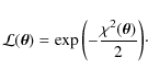
The
 function for
 data is

where
 is the measured value,
 is the hypothesised value for both a certain model and the parameters
 ,
and
,
and  is the known variance of the measurement.
For example,
and
represent
the measured and calculated B/C ratios.
is the known variance of the measurement.
For example,
and
represent
the measured and calculated B/C ratios.
The link between the target function, i.e., the posterior PDF of the parameters, and the experimental data is established with the help of Eqs. (11) to (13). This link guarantees the proper sampling of the parameter space using Markov chains, which spend more time in more relevant regions of parameter space, as described above.
3.3.2 Trial function
Despite the effectiveness of the Metropolis-Hastings algorithm, to optimise the efficiency of the MCMC and minimise the number of chains to be processed, trial functions should be as close as possible to the true distributions. We use a sequence of three trial functions to explore the parameter space. The first step is a coarse determination of the parameter PDF. This allows us to calculate the covariance matrix leading to a better coverage of parameter space, provided that the target PDF is sufficiently close to being an N-dimensional Gaussian. The last step takes advantage of a binary-space partitioning (BSP) algorithm.
Gaussian step
For the first iteration, the proposal density
 ,
required to obtain the trial value
from
is written as
,
required to obtain the trial value
from
is written as
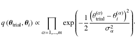
These represent m independent Gaussian distributions centred on
.
The distribution is symmetric, so that the acceptance
probability a follows Eq. (6).
The variance
 for each parameter is to be specified.
Each parameter
for each parameter is to be specified.
Each parameter
 is hence calculated to be

where x is a random number obeying a Gaussian distribution centred on zero with unit variance.
It is important to choose an optimal width
 to sample properly the posterior (target) distribution.
If the width is too large, as soon as the chain reaches a region of
high probability, most of the trial parameters fall into
a region of low probability and are rejected, leading to
a low acceptance and a long correlation length.
Conversely, for too small a width, the chain will take a longer time
to reach the interesting regions. Eventually, even if the chain
reaches these regions of high acceptance, only a partial
coverage of the PDF support will be sampled (also leading to
a long correlation length).
to sample properly the posterior (target) distribution.
If the width is too large, as soon as the chain reaches a region of
high probability, most of the trial parameters fall into
a region of low probability and are rejected, leading to
a low acceptance and a long correlation length.
Conversely, for too small a width, the chain will take a longer time
to reach the interesting regions. Eventually, even if the chain
reaches these regions of high acceptance, only a partial
coverage of the PDF support will be sampled (also leading to
a long correlation length).
In practice, we first define
(
)
equal to the expected range of the parameter. In a subsequent iteration,
is set to be
 times
times
 ,
i.e. the FWHM of the PDF obtained with the
first iteration. The result is actually insensitive to the numerical factor used.
,
i.e. the FWHM of the PDF obtained with the
first iteration. The result is actually insensitive to the numerical factor used.
Covariance matrix
The proposal density is taken to be an N-dimensional Gaussian of covariance
matrix V
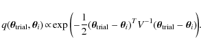
The covariance matrix V is symmetric and diagonalisable (D is a diagonal matrix of eigenvalues and P represents the change in the coordinate matrix),
and where again Eq. (6) holds. The parameters
are hence found to be

where
 is a vector of m random numbers following
a Gaussian distribution centred on zero and with unit variance.
is a vector of m random numbers following
a Gaussian distribution centred on zero and with unit variance.
The covariance matrix V is estimated, e.g., from a previous iteration using the Gaussian step. The advantage of this trial function with respect to the previous one is that it takes account of the possible correlations between the m parameters of the model.
Binary space partitioning (BSP)
A third method was developed to define a proposal density for which the results of the Gaussian step or the covariance matrix iterations are used to subdivide the parameter space into boxes, in each of which a given probability is affected.
The partitioning of the parameter space can be organised using a binary-tree data structure known as a binary-space partitioning tree (de Berg et al. 2000). The root node of the tree is the m-dimensional box corresponding to the entire parameter space. The binary-space partitioning is then performed by dividing each box recursively into two child boxes if the partitioning satisfies the following requirement: a box is divided only if the number of independent samples contained in this box is higher than a certain number (here we used a maximum of between 3% and 0.1% of the total number of independent samples). When a box has to be divided, the division is made along the longer side of the box (the box-side lengths are defined relative to the root-box sides). For each end node (i.e. node without any children), a probability, defined as the fraction of the number of independent samples in the box to their total number, is assigned. For empty boxes, a minimum probability is assigned and all the probabilities are renormalised so that the sum of all end-node probabilities equals 1.
The proposal density
 is then defined, in each
end-node box, as a uniform function equal to the assigned probability.
The sampling of this proposal density is simple and efficient:
an end node is chosen with the assigned probability
and the trial parameters are chosen uniformly in the corresponding box.
In comparison to the other two proposal densities, this
proposal density based on a BSP is asymmetric, because it is
only dependent on the proposal state
.
Hence, Eq. (4) must be used.
is then defined, in each
end-node box, as a uniform function equal to the assigned probability.
The sampling of this proposal density is simple and efficient:
an end node is chosen with the assigned probability
and the trial parameters are chosen uniformly in the corresponding box.
In comparison to the other two proposal densities, this
proposal density based on a BSP is asymmetric, because it is
only dependent on the proposal state
.
Hence, Eq. (4) must be used.
4 Implementation in the propagation model
The MCMC with the three above methods
are implemented in the USINE package![]() , which
computes the propagation of Galactic CR nuclei and anti-nuclei for
several propagation models (LBM, 1D and 2D diffusion models). The reader is referred to Maurin et al. (2001)
for a detailed description for the nuclear parameters (fragmentation and
absorption cross-sections), energy losses (ionisation and Coulomb), and
solar modulation (force-field) used.
, which
computes the propagation of Galactic CR nuclei and anti-nuclei for
several propagation models (LBM, 1D and 2D diffusion models). The reader is referred to Maurin et al. (2001)
for a detailed description for the nuclear parameters (fragmentation and
absorption cross-sections), energy losses (ionisation and Coulomb), and
solar modulation (force-field) used.
We briefly describe how the MCMC algorithm is implemented in the propagation part (Sect. 4.1), using a LBM - the procedure would be similar for any other model. The LBM and its parameters are briefly discussed (Sect. 4.2) as well as the input spectrum parameters (Sect. 4.3). Additional information about the data are gathered in Appendix B.
4.1 Flow chart
A flow chart of the Metropolis-Hastings MCMC algorithm used in the context of GCRs is given in Fig. 1.
![\begin{figure}
\par\includegraphics[width = 8.8cm]{0824fig1.eps}
\end{figure}](/articles/aa/full_html/2009/15/aa10824-08/img93.png) |
Figure 1:
Flow chart of the implemented MCMC algorithm:
|
| Open with DEXTER | |
 is the target function given
by Eq. (
is the target function given
by Eq. ( are chosen randomly in their expected range to crank up each Markov chain.
The interstellar (IS) CR fluxes are then calculated for this set
of parameters (see, e.g., Fig. 1 in
Maurin et al. 2002, for further details of the propagation steps).
The IS flux is modulated with the force-field approximation and the
resulting top-of-atmosphere (TOA) spectrum is compared with the data,
which allows us to calculate the
value
(Eq. (13)), hence the likelihood
(Eq. (12)).
This likelihood (in practice the log-likelihood)
is used to compute the acceptance probability (Eq. (4))
of the trial vector of parameters
(as generated by
one of the three trial functions described in Sect. 3.3.2).
Whether the trial vector is accepted or rejected implies whether
are chosen randomly in their expected range to crank up each Markov chain.
The interstellar (IS) CR fluxes are then calculated for this set
of parameters (see, e.g., Fig. 1 in
Maurin et al. 2002, for further details of the propagation steps).
The IS flux is modulated with the force-field approximation and the
resulting top-of-atmosphere (TOA) spectrum is compared with the data,
which allows us to calculate the
value
(Eq. (13)), hence the likelihood
(Eq. (12)).
This likelihood (in practice the log-likelihood)
is used to compute the acceptance probability (Eq. (4))
of the trial vector of parameters
(as generated by
one of the three trial functions described in Sect. 3.3.2).
Whether the trial vector is accepted or rejected implies whether
 or
or
 .
This procedure is repeated for the N steps of the chain. Obviously,
when
,
the propagation step does not
need to be repeated. Because of the nature of the MCMC algorithm, several chains can
be executed in parallel. Once completed, these chains are analysed (see
Sect. 3.2) - discarding the first step belonging
to the burning length and thinned according to the correlation length
l (Eq. (8)) - and combined to recover the
desired posterior PDF
.
.
This procedure is repeated for the N steps of the chain. Obviously,
when
,
the propagation step does not
need to be repeated. Because of the nature of the MCMC algorithm, several chains can
be executed in parallel. Once completed, these chains are analysed (see
Sect. 3.2) - discarding the first step belonging
to the burning length and thinned according to the correlation length
l (Eq. (8)) - and combined to recover the
desired posterior PDF
.
In this procedure, the user must decide i) the data to be used; ii)
the observable to retain in calculating the likelihood; and iii) the number of
free parameters m (of the vector
)
for which we seek the posterior
PDF.
4.2 Leaky-Box Model (LBM)
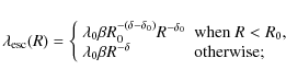
The LBM assumes that all CR species are confined
within the Galaxy with an escape rate that equals
 ,
where the escape
time
,
where the escape
time
 is rigidity-dependent, and is written as
 .
This escape time has two origins.
First, CRs can leak out the confinement volume and leave the Galaxy.
Second, they can be destructed by spallation on interstellar matter nuclei.
This latter effect is parameterised by the grammage x (usually expressed
in g cm-2), defined as the column density of
interstellar matter encountered by a path followed by a CR.
The CRs that reach Earth have followed different paths,
and can therefore be described by a grammage distribution
.
This escape time has two origins.
First, CRs can leak out the confinement volume and leave the Galaxy.
Second, they can be destructed by spallation on interstellar matter nuclei.
This latter effect is parameterised by the grammage x (usually expressed
in g cm-2), defined as the column density of
interstellar matter encountered by a path followed by a CR.
The CRs that reach Earth have followed different paths,
and can therefore be described by a grammage distribution
 .
The LBM assumes that
.
The LBM assumes that
 |
(16) |
where the mean grammage
 is related to the mass m, velocity v and escape time
by means of
is related to the mass m, velocity v and escape time
by means of
The function
 determines the amount of spallations
experienced by a primary species, and thus determines the secondary-to-primary
ratios, for instance B/C. From an experimentalist point of view,
is a quantity that can be inferred from measurements of
nuclei abundance ratios. The grammage
is known
to provide an effective description of diffusion
models (Berezinskii et al. 1990): it can be related to the
efficiency of confinement (which is determined by the diffusion coefficient and
to both the size and geometry of the diffusion volume), spallative destruction (which
tends to shorten the average lifetime of a CR and thus lower
determines the amount of spallations
experienced by a primary species, and thus determines the secondary-to-primary
ratios, for instance B/C. From an experimentalist point of view,
is a quantity that can be inferred from measurements of
nuclei abundance ratios. The grammage
is known
to provide an effective description of diffusion
models (Berezinskii et al. 1990): it can be related to the
efficiency of confinement (which is determined by the diffusion coefficient and
to both the size and geometry of the diffusion volume), spallative destruction (which
tends to shorten the average lifetime of a CR and thus lower
 ), and a mixture of other processes (such as convection,
energy gain, and losses).
), and a mixture of other processes (such as convection,
energy gain, and losses).
In this paper, we compute the fluxes in the framework of the
LBM with minimal reacceleration by the interstellar
turbulence, as described in Osborne & Ptuskin (1988) and Seo & Ptuskin (1994).
The grammage
is parameterised as
where we allow for a break, i.e. a different slope below and above a critical rigidity R0. The standard form used in the literature is recovered by setting
 .
For the entire set of n nuclei, a series of n equations
(see Maurin et al. 2001, for more details) for
the differential densities
.
For the entire set of n nuclei, a series of n equations
(see Maurin et al. 2001, for more details) for
the differential densities
 are solved
at a given kinetic energy per nucleon Ek/n (E is the
total energy), i.e.
are solved
at a given kinetic energy per nucleon Ek/n (E is the
total energy), i.e.
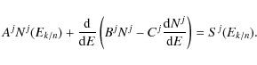
In this equation, the r.h.s. term is the source term that takes into account the primary contribution (see Sect. 4.3), the spallative secondary contribution from all nuclei k heavier than j, and the
 -decay of radioactive nuclei into j. The
first energy-dependent factor Aj is given by
-decay of radioactive nuclei into j. The
first energy-dependent factor Aj is given by

The two other terms correspond to energy losses and first-order reacceleration for Bj and to second-order reacceleration for Cj. Following Osborne & Ptuskin (1988) and Seo & Ptuskin (1994),

where
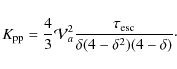
The strength of the reacceleration is mediated by the pseudo Alfvénic speed
 of the scatterers in units of km s-1 kpc-1.
This is related to a true speed given in a diffusion model with a thin
disk h and a diffusive halo L by means of
can be directly transposed and compared to a true speed Va,
as obtained in diffusion models.
of the scatterers in units of km s-1 kpc-1.
This is related to a true speed given in a diffusion model with a thin
disk h and a diffusive halo L by means of
can be directly transposed and compared to a true speed Va,
as obtained in diffusion models.
To summarise, our LBM with reacceleration may involve up to five
free parameters, i.e. the normalisation  ,
the slopes
,
the slopes  and
below or above the cut-off rigidity R0,
and a pseudo-Alfvén velocity
related to
the reacceleration strength.
and
below or above the cut-off rigidity R0,
and a pseudo-Alfvén velocity
related to
the reacceleration strength.
4.3 Source spectra
We assume that the primary source spectrum Qj(E) for
each nuclear species j is given by ( )
)
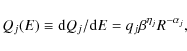
where qj is the source abundance,
 is the slope of the species j,
and the term
is the slope of the species j,
and the term
 manifests our ignorance about the low-energy spectral shape.
We further assume that
manifests our ignorance about the low-energy spectral shape.
We further assume that
 for all j,
and unless stated otherwise,
for all j,
and unless stated otherwise,
 in order to recover
d
in order to recover
d
 ,
as obtained from acceleration models (e.g., Jones 1994).
The constraints existing on
,
as obtained from acceleration models (e.g., Jones 1994).
The constraints existing on  are explored in Sect. 5.3.
The pattern of the source abundances observed in the cosmic radiation differs from that of the solar system. This is due to a segregation mechanism during the acceleration stage. Two hypotheses are disputed in the literature: one is based on the CR composition controlled by volatility and mass-to-charge ratio (Meyer et al. 1997; Ellison et al. 1997), and the other one is based on the first ionisation potential (FIP) of nuclei (e.g., Cassé & Goret 1973). In this work, for each configuration, the source abundances are initialised to the product of the solar system abundances (Lodders 2003), and the value of the FIP taken from Binns et al. (1989). The final fluxes are obtained by an iterative calculation of the propagated fluxes, rescaling the element abundances - keeping fixed the relative isotopic abundances - to match experimental data at each step until convergence is reached (see Fig. 1 in Maurin et al. 2002, for further details). The result is thus insensitive to the input values (more details about the procedure are given in Appendix B.1).
The measurement of all propagated isotopic fluxes should
characterise all source spectra parameters completely, i.e.
the qj and
parameters should be free.
However, only element fluxes are available, which motivates the above
rescaling approach. In Sect. 5.3,
a few calculations are undertaken to determine self-consistently,
along with the propagation parameters, i)
and ;
and ii)
the source abundances for the primary species C, O, and the mixed N elements
(the main contributors to the boron flux).
5 Results
We first examine the relative merits of four different parameterisations
of the LBM, and determine the statistical significance of adding more parameters. These models
correspond to
 with
with
- Model I
 ,
i.e. no reacceleration (
,
i.e. no reacceleration (
 )
and no break in the spectral index (
).
)
and no break in the spectral index (
).
- Model II
 ,
i.e. no critical rigidity (R0 = 0) and no break in the spectral index (
).
,
i.e. no critical rigidity (R0 = 0) and no break in the spectral index (
).
- Model III
 ,
i.e. no break in the spectral index (
).
,
i.e. no break in the spectral index (
).
- Model IV
 .
.
 data alone.
We also consider additional free parameters (Sect. 5.3) related to the source spectra, for a self-consistent determination of the propagation and source properties. Since we show that a break in the slope (Model IV) is not required by current data, we focus on Model III (for the description of the propagation parameters), defining:
- Model III+1
 ,
where the source slope
is a free parameter.
,
where the source slope
is a free parameter.
- Model III+2
 ,
where both the source slope
and the exponent
(of ,
see Eq. (20))
are free parameters.
,
where both the source slope
and the exponent
(of ,
see Eq. (20))
are free parameters.
- Model III+4
 ,
where the abundances qi of the most significantly contributing elements are also free parameters.
,
where the abundances qi of the most significantly contributing elements are also free parameters.
- Model III+5
 .
.
More details about the practical use of the trial functions can be found in Appendix C. In particular, the sequential use of the three sampling methods (Gaussian step, covariance matrix step, and then binary-space partitioning) is found to be the most efficient: all results presented hereafter are based on this sequence.
5.1 Fitting the B/C ratio
5.1.1 HEAO-3 data alone
We first constrain the model parameters with HEAO-3 data only (Engelmann et al. 1990). These data are the most precise data available at the present day for the stable nuclei ratio B/C of energy between 0.62 to 35 GeV/n.
The results for the models I, II, and III are presented in Figs. C.2, 2 top, and 2 bottom. The inner and outer contours are taken to be regions containing 68% and 95% of the PDF respectively (see Appendix A.1).
![\begin{figure}
\par\includegraphics[width = 8.8cm]{0824fig2a.eps}\vspace{3mm}
\includegraphics[width = 8.8cm]{0824fig2b.eps}
\end{figure}](/articles/aa/full_html/2009/15/aa10824-08/img134.png) |
Figure 2: Posterior distributions for Model II ( top) and Model III ( bottom) using HEAO-3 data only. For more details, refer to caption of Fig. C.2. |
| Open with DEXTER | |
As seen in Fig. 2, a more complicated shape for the different
parameters is found for Model II (top panel), and even more so for Model III (bottom panel).
This induces a longer correlation length (1.5 and 6.9 steps instead of 1 step) and
hence reduces the efficiency of the MCMC (75% for model II and 17% for model III).
Physically, the correlation between the parameters, as seen most clearly in Fig. 2 (bottom),
is understood as follows. First, ,
R0, and
are positively correlated.
This originates in the low-energy relation
 ,
which should remain approximately constant to reproduce the bulk of the data at GeV/n energy.
Hence, if R0 or
is increased, also increases to balance the product. On the other hand,
is negatively correlated
with
(and hence with all the parameters): this is the standard result that
to reach smaller
(for instance to reach a Kolmogorov spectrum), more
reacceleration is required. This can also be seen from Eq. (19),
where at constant
,
,
which should remain approximately constant to reproduce the bulk of the data at GeV/n energy.
Hence, if R0 or
is increased, also increases to balance the product. On the other hand,
is negatively correlated
with
(and hence with all the parameters): this is the standard result that
to reach smaller
(for instance to reach a Kolmogorov spectrum), more
reacceleration is required. This can also be seen from Eq. (19),
where at constant
,
 ,
where f is a decreasing function of :
hence, if
decreases,
,
where f is a decreasing function of :
hence, if
decreases,
 increases, and
then has to increase to retain the balance.
increases, and
then has to increase to retain the balance.
The values for the maximum of the PDF for the propagation parameters along with their 68% confidence intervals (see Appendix A) are listed in Table 1.
Table 1: Most probable values of the propagation parameters for different models, using B/C data (HEAO-3 only).
The values obtained for our Model I are in fair agreement with those derived by Webber et al. (1998), who found
could be related to the
fact that Webber et al. (1998) rely on a mere eye inspection to extract
the best-fit solution or/and use a different set of data. For example, comparing
Model I with a combination of HEAO-3 and low-energy data (ACE+Voyager 1 & 2+IMP7-8, see
Sect. 5.1.2) leads to
The reacceleration mechanism was invoked in the literature to decrease the spectral index toward its preferred value of 1/3 given by a Kolmogorov spectrum of turbulence. In Table 1,
the estimated propagation parameter values for the models II and III are indeed slightly smaller than
for Model I, but the Kolmogorov spectral index is excluded for all of these three cases (using HEAO-3 data only).
This result agrees with the findings of Maurin et al. (2001), in which a more realistic
two-dimensional diffusion model with reacceleration and convection was used.
We note that the values for
 km s-1 kpc-1, should lead to
a true speed
km s-1 kpc-1, should lead to
a true speed
![]() km s-1 in a diffusion
model for which the thin disk
half-height is h=0.1 kpc and the halo size is L=10 kpc: this is
consistent with values found in Maurin et al. (2002).
km s-1 in a diffusion
model for which the thin disk
half-height is h=0.1 kpc and the halo size is L=10 kpc: this is
consistent with values found in Maurin et al. (2002).
The final column in Table 1 indicates, for each model, the
best value per degree of freedom,
 d.o.f. This allows us to compare the relative merit of the models.
LB models with reacceleration reproduce the HEAO-3 data more accurately (with /d.o.f. of 1.43 and 1.30 for the Models
II and III respectively compared to /d.o.f. = 4.35
for Model I). The best-fit model B/C fluxes are shown with the
B/C HEAO-3 data modulated at
d.o.f. This allows us to compare the relative merit of the models.
LB models with reacceleration reproduce the HEAO-3 data more accurately (with /d.o.f. of 1.43 and 1.30 for the Models
II and III respectively compared to /d.o.f. = 4.35
for Model I). The best-fit model B/C fluxes are shown with the
B/C HEAO-3 data modulated at  MV in Fig. 3.
![\begin{figure}
\par\includegraphics[width = 8.5cm]{0824fig3.eps}
\end{figure}](/articles/aa/full_html/2009/15/aa10824-08/img154.png) |
Figure 3:
Best-fit ratio for Model I (blue dotted), II (red dashed), and
Model III (black solid) using the HEAO-3 data only (green symbols). The curves are
modulated with
|
| Open with DEXTER | |
at low energy can be related to convection in diffusion models (Jones 1979). Hence, it
is a distinct process as reacceleration.
The fact that Model III performs more successfully than Model II implies that both processes
are significant, as found in Maurin et al. (2001).
In the following, we no longer consider Model I and II, and inspect instead, the parameter dependence of Model III on the dataset selected.
5.1.2 Additional constraints from low-energy data
The actual data sets for the B/C ratio (see, e.g., Fig. 5)
show a separation into two energy domains: the low-energy
range extends from 10-2 GeV/n to 1 GeV/n
and the high-energy range goes from 1 GeV/n to
102 GeV/n. The spectral index
is
constrained by high-energy data, e.g., the HEAO-3 data,
and adding low-energy data allows us to more reliably constrain R0.
We note that by fitting only the low-energy data, only the grammage
crossed in very narrow energy domain would be constrained.
In a first step, we add only the ACE (CRIS) data (de Nolfo et al. 2006), which covers the energy range
from
 GeV/n to
 GeV/n, and which is later referred to as dataset B
(the dataset A being HEAO-3 data alone). The resulting posterior
distributions are similar for the datasets B and A (B is not shown, but A is given in Fig. 2, bottom).
Results for datasets A and B are completely consistent (first and second line of Table 2),
but for the latter, propagation parameters are more tightly constrained and the fit is improved
(
GeV/n, and which is later referred to as dataset B
(the dataset A being HEAO-3 data alone). The resulting posterior
distributions are similar for the datasets B and A (B is not shown, but A is given in Fig. 2, bottom).
Results for datasets A and B are completely consistent (first and second line of Table 2),
but for the latter, propagation parameters are more tightly constrained and the fit is improved
(
 /d.o.f. = 1.09). The ACE (CRIS) data are compatible with R0 = 0, but
the preferred critical rigidity is 2.47 GV.
/d.o.f. = 1.09). The ACE (CRIS) data are compatible with R0 = 0, but
the preferred critical rigidity is 2.47 GV.
All other low-energy data (ISEE-3, Ulysses, IMP7-8, Voyager 1 & 2, ACE) are then included (dataset D).
The resulting values of the propagation parameters are left unchanged. However, a
major difference lies in the higher
/d.o.f. of 4.15, which reflects an inconsistency
between the different low-energy data chosen for the MCMC. If the data point from the Ulysses experiment
is excluded,
/d.o.f. decreases to a value of 2.26, and
by excluding also the ISEE-3 data points (dataset C) it decreases further to 1.06
(see Table 2).
Table 2: Same as in Table 1, testing different B/C data sets.
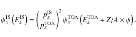
Since the set of low-energy data have different modulation parameters, the difference in the results for the various data subsets becomes clearer after the data have been demodulated. The force-field approximation provides a simple analytical one-to-one correspondence between the modulated top-of-the atmosphere (TOA) and the demodulated interstellar (IS) fluxes. For an isotope x, the IS and TOA energies per nucleon are related by (
(
 is the modulation parameter), and the fluxes
by (px is the momentum per nucleon of x)
is the modulation parameter), and the fluxes
by (px is the momentum per nucleon of x)
 |
(21) |
The B/C ratio results from a combination of various isotopes, and assuming the same Z/A for all isotopes, we find that
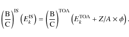 |
(22) |
The modulated and demodulated low-energy B/C data are shown in Fig. 4 (see caption for details). The ISEE-3 and Ulysses data points, as just underlined,
![\begin{figure}
\par\includegraphics[width = 8.5cm]{0824fig4.eps}
\end{figure}](/articles/aa/full_html/2009/15/aa10824-08/img174.png) |
Figure 4: HEAO-3 and ACE (CRIS) modulated (TOA, solid line) and demodulated (IS, dashed line) data points have been connected to guide the eye. Filled symbols (modulated and demodulated) correspond to HEAO-3, ACE (CRIS), IMP7-8 and Voyager 1 and 2. On the TOA curve, the empty red stars and the blue upper triangle correspond to ISEE-3 and Ulysses. |
| Open with DEXTER | |
 MV for
ISEE-3 and MV for Ulysses would be required. Significant uncertainties
MV for
ISEE-3 and MV for Ulysses would be required. Significant uncertainties
 GV are quoted in general, so that it is difficult to
conclude whether there are systematics in the measurement or if the modulation quoted
in the papers is inappropriate. Some experiments have also accumulated the signal for
several years, periods during which the modulation changes. It is beyond the
scope of this paper to discuss this issue further.
Below, we discard both ISEE-3 and Ulysses data in selecting an homogeneous
low-energy data set, which includes the most recent ACE (CRIS) data.
GV are quoted in general, so that it is difficult to
conclude whether there are systematics in the measurement or if the modulation quoted
in the papers is inappropriate. Some experiments have also accumulated the signal for
several years, periods during which the modulation changes. It is beyond the
scope of this paper to discuss this issue further.
Below, we discard both ISEE-3 and Ulysses data in selecting an homogeneous
low-energy data set, which includes the most recent ACE (CRIS) data.
Table 3: Best-fit parameters for selected models and B/C sets.
The resulting best-fit models, when taking low-energy data into account, are
displayed in Fig. 5. The B/C best-fit ratio is displayed for
Model III and the dataset A (red thin lines) and C (black thick lines). Model III-B
(not shown) yields similar results to Model III-C. Solid and dashed lines correspond
to the two modulations
MV (HEAO-3 and IMP7-8) and
 MV
respectively (ACE and Voyager 1 & 2). Although the fit from HEAO-3 alone provides a
good match at low energy, adding ACE (CRIS) and Voyager 1 & 2 constraints slightly
shifts all of the parameters to lower values.
MV
respectively (ACE and Voyager 1 & 2). Although the fit from HEAO-3 alone provides a
good match at low energy, adding ACE (CRIS) and Voyager 1 & 2 constraints slightly
shifts all of the parameters to lower values.
![\begin{figure}
\par\includegraphics[width = 8.5cm]{0824fig5.eps}
\end{figure}](/articles/aa/full_html/2009/15/aa10824-08/img183.png) |
Figure 5:
Best-fit B/C flux (Model III) for datasets A (thin red curves) and C
(thick black curves). Above 300 MeV/n, B/C is modulated to |
| Open with DEXTER | |
In a final try, we take into account all available data (dataset E,
final line of Table 2).
Many data are clearly inconsistent with each other (see Fig. 8), but as
for the low-energy case, although the
/d.o.f.
is worsened, the preferred values of the propagation parameters are not
changed drastically (compare with datasets B, C, and D in Table 2).
We await forthcoming data from CREAM, TRACER, and PAMELA to be able to confirm
and refine the results for HEAO-3 data.
5.1.3 Model IV: break in the spectral index
We have already mentioned that the rigidity cut-off
may be associated with the existence of a galactic wind
in diffusion models. By allowing a break to occur in the spectral
index of
(see Eq. (17)),
we search for a deviations from a single power law
(
 )
or from the cut-off case (
).
)
or from the cut-off case (
).
Adding a new parameter
(Model IV) increases the correlation length of
the MCMC, since R0 and
are correlated
(see Eq. (17)).
The acceptance
(Eq. (9)) is hence extremely low. For Model IV-C
(i.e. using dataset C, see Table 2),
we find
 .
The PDF for
is shown in the
left panel of Fig. 6. The most probable values and 68%
confidence intervals obtained are
.
The PDF for
is shown in the
left panel of Fig. 6. The most probable values and 68%
confidence intervals obtained are
![]() ,
which are consistent with values found for other models,
as given in Tables 1 and 2:
adding a low-energy spectral break only allows us to better adjust low-energy
data (figure not shown). The best-fit parameters, for which
,
which are consistent with values found for other models,
as given in Tables 1 and 2:
adding a low-energy spectral break only allows us to better adjust low-energy
data (figure not shown). The best-fit parameters, for which
 ,
are reported in Table 3. The small value of
(smaller than 1) may indicate an over-adjustment, which would disfavour the model.
,
are reported in Table 3. The small value of
(smaller than 1) may indicate an over-adjustment, which would disfavour the model.
It is also interesting to compel
to be positive, to check whether
(equivalent
to Model III),
(equivalent to Model II), or any
value in-between that is preferred. We find the most probable values to be
![]() .
The corresponding PDF for is shown in the right panel of Fig. 6. The maximum occurs for
,
which is also found to be the best-fit value; we checked that
the best-fit parameters matches those given in Table 3 for Model III-C.
A secondary peak appears at
.
The corresponding PDF for is shown in the right panel of Fig. 6. The maximum occurs for
,
which is also found to be the best-fit value; we checked that
the best-fit parameters matches those given in Table 3 for Model III-C.
A secondary peak appears at
 ,
such as
,
such as
 corresponding to Model II. The associated
for this configuration
is worse than that obtained with
,
in agreement with the conclusion
that Model III provides a closer description of the data than Model II.
corresponding to Model II. The associated
for this configuration
is worse than that obtained with
,
in agreement with the conclusion
that Model III provides a closer description of the data than Model II.
| |
Figure 6:
Marginalised PDF for
the low-energy spectral index |
| Open with DEXTER | |
 ( right panel).
5.1.4 Summary and confidence levels for the B/C ratio
In the previous paragraphs, we have studied several models and B/C datasets. The two main conclusions that can be drawn are i) the best-fit model is Model III, which includes reacceleration and a cut-off rigidity; and ii) the most likely values of the propagation parameters are not too dependent on the data set used, although when data are inconsistent with each other the statistical interpretation of the goodness of fit of a model is altered (all best-fit parameters are gathered in Table 3). The values of the derived propagation parameters are close to the values found in similar studies and the correlation between the LB transport parameters are well understood.
Taking advantage of the knowledge of the
distribution, we can extract
a list of configurations, i.e. a list of parameter sets, based on CLs of
the PDF (as explained in Appendix A.2). The distribution is shown for
our best model, i.e. Model III, in Fig. 7. The red and black areas correspond
to the 68% and 95% confidence intervals, which are used to generate two configuration lists,
from which 68% and 95% CLs on, e.g., fluxes, can be derived![]() .
.
![\begin{figure}
\par\includegraphics[width = 8.5cm]{0824fig7.eps}
\end{figure}](/articles/aa/full_html/2009/15/aa10824-08/img193.png) |
Figure 7:
|
| Open with DEXTER | |
The B/C best-fit curve (dashed blue), the 68% (red solid), and 95% (black solid) CL
envelopes are shown in Fig. 8.
For the specific case of the LBM, this demonstrates that current data are already
able to constrain strongly the B/C flux (as reflected by the
good value
 ), even at high energy.
This provides encouraging support in the discriminating power of forthcoming data.
However, this conclusion must be confirmed by analysis of a more refined model
(e.g., diffusion model), for which the situation might not be so simple.
), even at high energy.
This provides encouraging support in the discriminating power of forthcoming data.
However, this conclusion must be confirmed by analysis of a more refined model
(e.g., diffusion model), for which the situation might not be so simple.
![\begin{figure}
\par\includegraphics[width = 8.5cm]{0824fig8.eps}
\end{figure}](/articles/aa/full_html/2009/15/aa10824-08/img195.png) |
Figure 8:
Confidence regions of the B/C ratio for Model III-C as calculated from all
propagation parameters satisfying Eq. (A.2). The blue-dashed line is the best-fit
solution, red-solid line is 68% CL and black-solid line 95% CL. Two modulation parameters
are used: |
| Open with DEXTER | |
From the same lists, we can also derive the range allowed for the source abundances of elements (we did not try to fit isotopic abundances here, although this can be achieved, e.g., as in Simpson & Connell 2001, and references therein). The element abundances are gathered in Table 4, for elements from C to Si (heavier elements were not used in this study). They can be compared with those found in Engelmann et al. (1990) (see also those derived from Ulysses data, Duvernois et al. 1996). For some elements, the agreement is striking (F, Mg), and is otherwise fair. The difference for the main progenitors of boron, i.e. C, N, and O, is a bit puzzling, and is probably related to a difference in the input-source spectral shape. This is discussed further in Sect. 5.3, where we also determine self-consistently the propagation parameters along with the C, N, and O abundances.
Table 4: Element source abundances for Model III-C and comparison with HEAO-3 results.
5.2 Constraints from 
In the context of indirect dark-matter searches, the antimatter
fluxes (
,
 and e+) are used to look for
exotic contributions on top of the standard, secondary ones.
and e+) are used to look for
exotic contributions on top of the standard, secondary ones.
The standard procedure is to fit the propagation parameters
to B/C data, and apply these parameters in calculating the
secondary and primary (exotic) contributions.
The secondary flux calculated for our best-fit Model III-C is
shown, along with the data (see Appendix B.2 for
more details) in Fig. 9 (black-solid line).
For this model, we can calculate the value for the
data, and we find  d.o.f. = 1.86. The fit is not perfect, and
as found in other studies (e.g., Duperray et al. 2005),
the flux is somehow low at high energy (PAMELA data are awaited
to confirm this trend). However, we checked that these high-energy
data points are not responsible for the large value.
The latter could be attributed to either a small exotic contribution,
a different propagation history for species for which
A/Z=1 or
d.o.f. = 1.86. The fit is not perfect, and
as found in other studies (e.g., Duperray et al. 2005),
the flux is somehow low at high energy (PAMELA data are awaited
to confirm this trend). However, we checked that these high-energy
data points are not responsible for the large value.
The latter could be attributed to either a small exotic contribution,
a different propagation history for species for which
A/Z=1 or
 ,
or inaccurate data.
,
or inaccurate data.
It may therefore appear reasonable to fit directly the propagation parameters
to the
flux, assuming that it is a purely secondary species.
Since the fluxes of its progenitors (p and He) are well measured,
this should provide an independent check of the propagation history.
We first attempted to apply the MCMC method to the
data with Model III,
then Model II and finally Model I. However, even the simplest model exhibits
strong degeneracies, and the MCMC chains could not converge. We had to revert
to a model with no reacceleration (
), no critical rigidity
(R0 = 0), and no break in the spectral index (
), for which
![]() (hereafter Model 0).
The
(hereafter Model 0).
The  values found for the two parameters
 are
are
![]() and
and
![]() .
Hence, only one parameter ()
is required to reproduce
the data, as seen in Fig. 9 (red-dashed line,
.
Hence, only one parameter ()
is required to reproduce
the data, as seen in Fig. 9 (red-dashed line,
 d.o.f. = 1.128).
This is understood as follows: due to the combined effect of modulation and
the tertiary contribution (
inelastically interacting on the ISM, but
surviving as a
of lower energy), the true low-energy data points all
correspond to
produced at a few GeV energies. Due to
the large scattering in the data, it is sufficient to produce the correct
amount of
at this particular energy to account for all of the data.
d.o.f. = 1.128).
This is understood as follows: due to the combined effect of modulation and
the tertiary contribution (
inelastically interacting on the ISM, but
surviving as a
of lower energy), the true low-energy data points all
correspond to
produced at a few GeV energies. Due to
the large scattering in the data, it is sufficient to produce the correct
amount of
at this particular energy to account for all of the data.
![\begin{figure}
\par\includegraphics[width = 8cm]{0824fig9.eps}
\end{figure}](/articles/aa/full_html/2009/15/aa10824-08/img223.png) |
Figure 9:
Demodulated anti-proton data and IS flux for Model 0 (best fit on
|
| Open with DEXTER | |
Due to the importance of antimatter fluxes for indirect dark-matter
searches, this novel approach could be helpful in the future. However, this
would require a more robust statistics of the
flux, especially
at higher energy, to lift the degeneracy in the parameters.
5.3 Adding free parameters related to the source spectra
In all previous studies (e.g., Jones et al. 2001), the source parameters were investigated after the propagation parameters had been determined from the B/C ratio (or other secondary to primary ratio). We propose a more general approach, where we fit simultaneously all of the parameters. With the current data, this already provides strong constraints on the CR source slope
and source abundances (CNO).
Higher-quality data are awaited to refine this analysis.
We also show how this approach can help to uncover inconsistencies in the measured fluxes.
For all models below, taking advantage of the results obtained in Sect. 5.1,
we retain Model III-C. The roman number refers to the free transport parameters
of the model (III =
 ), and the capital refers to
the choice of the B/C dataset (C=HEAO-3+Voyager 1 & 2 + IMP7-8, see Table 2).
This is supplemented by source spectra parameters and additional data for the element
fluxes.
), and the capital refers to
the choice of the B/C dataset (C=HEAO-3+Voyager 1 & 2 + IMP7-8, see Table 2).
This is supplemented by source spectra parameters and additional data for the element
fluxes.
5.3.1 Source shape
and
from Eq. (20)
As a free parameter, we first add a universal source slope .
We then allow ,
parameterising a universal low-energy shape of all spectra,
to be a second free parameter.
In addition to B/C constraining the transport parameters, some primary species must
be added to constrain
and .
We restrict ourselves to O,
the most abundant boron progenitor, because it was measured by both the HEAO-3
experiment (Engelmann et al. 1990), and also the TRACER
experiment (Ave et al. 2008).
The modulation levels were MV for HEAO-3 and  MV for TRACER.
We estmated the latter number from the solar activity at the time of flight
(2 weeks in December 2003) as seen from neutron monitors
data
MV for TRACER.
We estmated the latter number from the solar activity at the time of flight
(2 weeks in December 2003) as seen from neutron monitors
data![]() .
.
In total, we test four models (denoted by 1a, 1b, 2a, and 2b for legibility):
- III-C+1a:
 ,
with O = HEAO-3;
,
with O = HEAO-3;
- III-C+1b:
,
with O=TRACER;
- III-C+2a:
 ,
with O = HEAO-3;
,
with O = HEAO-3;
- III-C+2b:
,
with O = TRACER.
 fixed to 2.65).
Table 5: Most probable values of the propagation and source parameters for different parameterisation of the source spectrum.
We remark that by adding HEAO-3 oxygen data to the fit (1a), the propagation parameters,
R0,
and
overshoot Model III-C's results, while they undershoot those of Model 1b (TRACER data).
The parameter
undershoots and overshoots for these two
models respectively, since it is anti-correlated with the former parameters.
As a consequence, the fit to B/C is worsened, especially at low energy
(see Fig. 10).
![\begin{figure}
\par\includegraphics[width = 8cm]{0824fig10.eps} %
\end{figure}](/articles/aa/full_html/2009/15/aa10824-08/img275.png) |
Figure 10:
B/C ratio from best-fit models of Table 6.
In addition to the propagation parameters, free parameters of the source spectra
are |
| Open with DEXTER | |
The top left panel of Fig. 11 shows the slopes
derived for
Models 1a (solid black) and 1b (dashed blue). In both cases, is well constrained, but the values are inconsistent, a result that is clear because
the low-energy data are also inconsistent: the demodulated (i.e. IS) HEAO-3 and TRACER
oxygen data points are shown in the right panel of Fig. 11.
![\begin{figure}
\par\mbox{\includegraphics[width = 4.2cm]{0824fig11a.eps}\include...
...24fig11b.eps} }
\par\includegraphics[width = 8.4cm]{0824fig11c.eps}
\end{figure}](/articles/aa/full_html/2009/15/aa10824-08/img276.png) |
Figure 11:
Marginalised PDF for models III-C+1 ( |
| Open with DEXTER | |
to be a free parameter (family of models III+2).
The net effect is to absorb any uncertainty originating in either the modulation level
or the source-spectrum low-energy shape. As shown in the bottom panel of Fig. 11,
the source slopes derived from the two experiments are now in far closer agreement (bottom left),
with
 .
The most probable values and the best-fit model values are
given in Tables 5 and 6 respectively. The
effect of this action is evident in the low-energy slope of the source
spectrum .
As seen in the bottom-right
panel, the two data sets contain significantly inconsistent ranges.
The value
.
The most probable values and the best-fit model values are
given in Tables 5 and 6 respectively. The
effect of this action is evident in the low-energy slope of the source
spectrum .
As seen in the bottom-right
panel, the two data sets contain significantly inconsistent ranges.
The value
 probably indicates that
the solar modulation we chose was incorrect. The value
probably indicates that
the solar modulation we chose was incorrect. The value
 might provide a reasonable guess of the low-energy shape of the source spectrum, but
might also be a consequence of systematics in the experiment. The associated
oxygen fluxes are shown in Fig. 12 for the best-fit models:
as explained, models that allow
to vary (thick lines) reproduce more accurately
the data than when
is set to be -1 (thin lines).
might provide a reasonable guess of the low-energy shape of the source spectrum, but
might also be a consequence of systematics in the experiment. The associated
oxygen fluxes are shown in Fig. 12 for the best-fit models:
as explained, models that allow
to vary (thick lines) reproduce more accurately
the data than when
is set to be -1 (thin lines).
![\begin{figure}
\par\includegraphics[width = 8.4cm]{0824fig12.eps} %
\end{figure}](/articles/aa/full_html/2009/15/aa10824-08/img280.png) |
Figure 12: Same models as in Fig. 10, but for the oxygen flux. |
| Open with DEXTER | |
Although it would be precipitate to draw any firm conclusion about the low-energy shape, we can turn the argument
around to serve as a diagnosis of the low-energy data quality. For instance,
assuming that the spectral index
of all elements was the same, extracting and comparing  for each of these i elements may enable us to infer some systematics
remaining in the data. It would be worth fitting the H and He species, which are the
most reliably measured fluxes to date; this will be considered in a future study
using diffusion models.
for each of these i elements may enable us to infer some systematics
remaining in the data. It would be worth fitting the H and He species, which are the
most reliably measured fluxes to date; this will be considered in a future study
using diffusion models.
5.3.2 ,
and source normalisation qi
The final two models add, as free parameters, the CNO element source abundances (relative isotopic abundances are fixed to SS ones). The data used in the fit are B/C, C, N, and O, all measured by HEAO-3 (TRACER data for C and N have not yet been published). The models, which are denoted by short 4a and 5a in the text below, are:
- III-C+4a:
 ;
;
- III-C+5a:
 .
.
![\begin{figure}
\par\includegraphics[width =17cm,clip]{0824fig13.eps}
\end{figure}](/articles/aa/full_html/2009/15/aa10824-08/img284.png) |
Figure 13: PDF (diagonal) and 2D correlations (off-diagonal) plots for the nine free parameters of Model III-C+5 when fitted on B/C, and CNO HEAO-3 data. |
| Open with DEXTER | |
 ),
even using the BSP trial function. To obtain 800 independent points,
a total
),
even using the BSP trial function. To obtain 800 independent points,
a total
 steps were completed. The contours are not as regular as for our 4-parameter
model (see Fig. 2), but correlations between the parameters
are still clearly evident: we recover the
steps were completed. The contours are not as regular as for our 4-parameter
model (see Fig. 2), but correlations between the parameters
are still clearly evident: we recover the
 correlations
(and anti-correlation with
). In addition, we note that
all source-related parameters (,
and element abundances
correlations
(and anti-correlation with
). In addition, we note that
all source-related parameters (,
and element abundances
 )
are correlated among themselves and with
(hence anti-correlated
with the remaining transport parameters). This is especially visible for the
primary species C and O, while less clear for the mixed species N.
This is understood as the parameter ,
i.e. the slope of the propagated
primary fluxes (
)
are correlated among themselves and with
(hence anti-correlated
with the remaining transport parameters). This is especially visible for the
primary species C and O, while less clear for the mixed species N.
This is understood as the parameter ,
i.e. the slope of the propagated
primary fluxes (
 )
is mostly fixed by measurements: if we decrease ,
then
must be
increased to match the data. However, if the source slope is increased,
the exponent
must also increase to match the low-energy data.
The positive correlation between source abundances comes from the
fact that relative fluxes should be preserved.
)
is mostly fixed by measurements: if we decrease ,
then
must be
increased to match the data. However, if the source slope is increased,
the exponent
must also increase to match the low-energy data.
The positive correlation between source abundances comes from the
fact that relative fluxes should be preserved.
The most probable values are gathered in Table 5.
Compared with the respective Models 1a and 2a, leaving
the source abundances  ,
,
 and
and  free in 4a and 5a
does not significantly change our conclusions. Again, adding (2a and 5a) as a free parameter allows us to absorb the
low-energy uncertainties in the data, so that we obtain
free in 4a and 5a
does not significantly change our conclusions. Again, adding (2a and 5a) as a free parameter allows us to absorb the
low-energy uncertainties in the data, so that we obtain
 (5a) instead of the biased value of 2.13 (4a). The same conclusions
hold for other propagation parameters. On the derived source
abundances, the impact of adding the parameter
is for them to increase.
The relative C:N:O abundances (
(5a) instead of the biased value of 2.13 (4a). The same conclusions
hold for other propagation parameters. On the derived source
abundances, the impact of adding the parameter
is for them to increase.
The relative C:N:O abundances ( )
are respectively 0.78:0.36:1 (4a) and 0.82:0.40:1 (5a), the second
model providing values slightly closer to those derived from HEAO-3 data 0.81:0.49:1.
)
are respectively 0.78:0.36:1 (4a) and 0.82:0.40:1 (5a), the second
model providing values slightly closer to those derived from HEAO-3 data 0.81:0.49:1.
The difference in the source element abundances when they are rescaled to match the
data or including them in the MCMC is also seen from Table 6,
which gathers the best-fit parameters. The next-to-last line reproduces
obtained
for all models: all abundances are roughly in agreement, although our approach
underlines the importance of taking the correlations between the parameters
properly into account in extracting unbiased estimates of the propagation and
source parameters.
Table 6: Best-fit values of propagation and source parameters using B/C and CNO data for models as given in Table 5.
The goodness of fit for the models when applied to the B/C, C, N, and O data is shown in
the last column of Table 6, in terms of the
value. The models in which
is free do not provide a closer match between
models and data but also a no poorer fit than when
is fixed.
As soon as primary fluxes are included in the fit
(compared to Model III-C), the
is worsened.
This is due to a combination of an imperfect fit to the primary fluxes and,
as already said, a poorer B/C fit because the propagation parameters are
optimised to match the former rather than the latter (B/C). The best-fit parameters are given in the
same Table, and the associated CNO fluxes are plotted in Fig. 14
for illustration purposes.
![\begin{figure}
\par\mbox{\includegraphics[width = 2.6cm]{0824fig14a.eps}\include...
...]{0824fig14b.eps}\includegraphics[width = 2.6cm]{0824fig14c.eps} }\end{figure}](/articles/aa/full_html/2009/15/aa10824-08/img305.png) |
Figure 14: Carbon, nitrogen and oxygen fluxes from best-fit models of Table 6. |
| Open with DEXTER | |
5.3.3 Perspective on source spectrum parameters
Other primary species could have been included in the
calculation to
i) constrain further ;
and/or ii) to check the hypothesis
for different species; and/or iii) diagnose some problems in the data, if we believe
the slope should be universal.
However, using a few primary species (O or CNO) already affects
the goodness of fit of B/C (compare model III-C to others in Fig. 10).
Since there are many more measured primary fluxes than secondary
ones, taking too many primaries would weigh too significantly in the ,
compared to the B/C contribution, and this would divert the MCMC into regions of
the parameter space that fit these fluxes rather than B/C. Since systematic errors
are known to be larger in flux
measurements than in ratios, this may lead to biased estimates of the propagation parameters.
Allowing
to be a free parameter is a first step to decrease the impact
of this bias (in the low-energy part of the spectrum).
These biases are not necessarily an issue since we may be more
interested in estimates of the source parameters rather than in unbiased
value of the propagation parameters.
To illustrate the difficulty in data systematics, it suffices to say that for the most abundant species H and He, all experiments provided mutually incompatible measurements, until AMS and BESS experiments flew ten years ago. We cannot therefore expect HEAO-3 data, acquired in 1979, to be completely free of such drawbacks. Again, we await the publication of several forthcoming new data sets before pursuing our analysis further in this direction.
6 Conclusion
We have implemented a Markov Chain Monte Carlo to extract the posterior distribution functions of the propagation parameters in a LBM. Three trial functions were used, namely a standard Gaussian step, an N-dimensional Gaussian step and its covariance matrix, and a binary-space partitioning. For each method, a large number of chains were processed in parallel to accelerate the PDF calculations. The three trial functions were used sequentially, each method providing some inputs to the next: while the first one was good at identifying the general range of the propagation parameters, it was not as efficient in providing an accurate description of the PDF. The two other methods provided this accuracy, and the final results were based on PDF obtained from the chains processed with the binary-space partitioning.
Taking advantage of the sound statistical properties of the MCMC, confidence intervals for the
propagation parameters can be given, as well as confidence contours for all fluxes
and other quantities derived from the propagation parameters. The MCMC was also used
to compare the impact of choosing different datasets and ascertain the merits of
different hypotheses concerning the propagation models.
Concerning the first aspect, we have shown that combining different B/C datasets leaves
mostly unchanged the propagation parameters, while strongly affecting the assessment
of the goodness of a model. We also show that at present, the
data do not cover
a sufficiently large energy range to constrain the propagation parameters, but they
could be useful in crosschecking the secondary nature of the flux in the future.
In this first paper, we have focused on the phenomenologically well-understood LBM,
to ease and simplify the discussion and implementation of the MCMC. In agreement with
previous studies, we confirm that a model with a rigidity cutoff performs more successfully
than one without and that reacceleration is preferred over no reacceleration. Such a model
can be associated with a diffusion model with wind and reacceleration. As found in
Maurin et al. (2001), the best-fit models demand both a rigidity cutoff (wind)
and reacceleration, but do not allow us to reconcile the diffusion slope
with a Kolmogorov spectrum for turbulence. An alternative
model with two slopes for the diffusion was used, but it is not favoured by the data.
In a last stage, we allowed the abundance and slope of the source spectra to be free
parameters, as well as the element abundances of C, N, and O. This illustrated a
correlation between the propagation and source parameters, potentially biasing the
estimates of these parameters. The best-fit model slope for the source abundances
was
 using HEAO-3 data, compatible with
the value
using HEAO-3 data, compatible with
the value
 for TRACER data. The MCMC approach allowed us
to draw confidence intervals for the propagation parameters, the source parameters,
and also for all fluxes.
for TRACER data. The MCMC approach allowed us
to draw confidence intervals for the propagation parameters, the source parameters,
and also for all fluxes.
A wealth of new data on Galactic CR fluxes are expected soon. As illustrated for the LBM, the MCMC is a robust tool in handling complex data and model parameters, where one has to fit simultaneously all source and propagation parameters. The next step is to apply this approach to more realistic diffusion models and larger datasets, on a wider range of nuclear species.
Acknowledgements
D.M. and R.T. warmly thank Joanna Dunkley for useful discussions at an early stage of this work. We thank Céline Combet for a careful reading of the paper.
Appendix A: Best fit, goodness of a model, most probable values and confidence levels/intervals
The best-fit model parameters are given by a unique set of parameters for which the value of Eq. (13) is minimized;
the goodness of fit of a model is given by
d.o.f.
On the other hand, the most probable value for each parameter  is defined as the maximum
 of its PDF (after marginalising).
The most probable
of its PDF (after marginalising).
The most probable
 and best-fit model parameters
 do not necessarily coincide, especially when correlations exist between parameters.
The best-fit model parameters are best suited to providing the most likely
CR fluxes, whereas the 1D marginalised PDF provides directly the most likely value
of the parameter.
do not necessarily coincide, especially when correlations exist between parameters.
The best-fit model parameters are best suited to providing the most likely
CR fluxes, whereas the 1D marginalised PDF provides directly the most likely value
of the parameter.
A.1 Confidence levels/intervals on parameters
Confidence intervals (CI), associated with a confidence level (CL), are
constructed from the PDF.
The asymmetric interval
![]() such as
such as
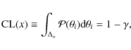 |
(A.1) |
defines the
 confidence level (CL), along with the CI of the
parameter .
Here, the CIs (i.e.
confidence level (CL), along with the CI of the
parameter .
Here, the CIs (i.e.
 and
and
 )
are found by decreasing the value
)
are found by decreasing the value
 from
from
 to
to
 ,
such that
,
such that
 .
This is easily generalised to 2D confidence levels in constructing
2D confidence intervals as shown later in correlation plots. Below, we use the
.
This is easily generalised to 2D confidence levels in constructing
2D confidence intervals as shown later in correlation plots. Below, we use the
 and
and  CLs, corresponding to
and
CLs, corresponding to
and  uncertainties.
A.2 Confidence intervals on fluxes
The best-fit model fluxes (e.g., B/C, O, )
are calculated
from the best-fit model parameters. Confidence levels in these quantities
cannot be obtained from the 1D marginalised CIs of the
parameters. They must be constructed from
a sampling of the (still) correlated parameters. This is achieved
by using all sets of parameters
![]() ,
for which
,
for which
 falls in the
  confidence level of the
PDF.
Once these sets are found, we simply calculate the desired flux for all
the sets: the maximum and minimum values are kept for each energy bin, defining
confidence envelopes for this flux. Thus, the main task is to construct
confidence intervals for the distribution.
confidence level of the
PDF.
Once these sets are found, we simply calculate the desired flux for all
the sets: the maximum and minimum values are kept for each energy bin, defining
confidence envelopes for this flux. Thus, the main task is to construct
confidence intervals for the distribution.
For n parameters in the large sample limit - where the joint PDF for
the estimator of the parameters and the likelihood function become Gaussian -,
the CI is given by
![\begin{displaymath}[\chi^2_{{\rm min}},~ \chi^2_{{\rm min}}+\Delta \chi^2], \quad
{\rm where} \quad \Delta \chi^2 = Q_{\gamma} (1 - \gamma, n)
\end{displaymath}](/articles/aa/full_html/2009/15/aa10824-08/img327.png)
is the quantile of order
(confidence level CL) of the distribution (Cowan 1997).
However, by applying the MCMC, we have access to a direct sampling of the
distribution. Hence, independently of the statistical meaning of a model,
the confidence interval is extracted from the cumulative PDF,
by requiring that
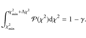
We nevertheless checked that both approaches provide similar results. For instance, the CIs (for Model III-C) obtained directly from Fig. 7 are
 quantiles (Cowan 1997).
Appendix B: Data
In the paper, we focus on the B/C ratio, which is the most accurate
tracer of the propagation parameters (other tracers, such
as the sub-Fe/Fe or the quartet 1H, 2H, 3He and 4He
are not considered). We also estimate the potential
of the
,
a secondary species, as an alternative species
for constraining these parameters. We describe below the typical
configurations used to calculate the corresponding spectrum
as well as the associated datasets used.
B.1 B/C
The default configuration for nuclei is the following: the value of the observed propagated slope,
unless stated otherwise,
is set to be 2.65 (Ave et al. 2008), and source abundances
of the most abundant species (C, N, O, F, Ne, Na, Mg, Al, Si) are
rescaled to match HEAO-3 data at 10.6 GeV/n. Boron is assumed to be a
pure secondary species. Only elements lighter than Si are propagated,
since they are the only relevant ones for determining B/C (Maurin et al. 2001).
For B/C at intermediate GeV energies, we use HEAO-3 data (Engelmann et al. 1990). A collection of low-energy data is formed by data sets for the IMP7-8 (Garcia-Munoz et al. 1987), ISEE-3 (Krombel & Wiedenbeck 1988), Ulysses (Duvernois et al. 1996), and Voyager 1&2 (Lukasiak et al. 1999), and ACE (CRIS) (de Nolfo et al. 2006) spacecrafts. At higher energy, we consider balloon flights (Lezniak & Webber 1978; Simon et al. 1980; Orth et al. 1978; Dwyer & Meyer 1987), the ATIC-2 balloon-borne experiment (Panov et al. 2007), and the Spacelab-2 experiment (Mueller et al. 1991). For element fluxes, HEA0-3 and TRACER results (Ave et al. 2008) are used.
B.2
For the calculation of the
flux, the situation is simpler:
the production of this secondary flux can be directly linked to the accurate
measurements of propagated p and He fluxes, by the
AMS (Alcaraz et al. 2000b; AMS Collaboration et al. 2000; Alcaraz et al. 2000a)
and BESS experiments (Shikaze et al. 2007; Sanuki et al. 2000).
For more details of the
flux calculation (cross sections,
source terms, ...), the reader is referred to Donato et al. (2001).
For the
data, we consider the AMS 98 (AMS Collaboration et al. 2002)
experiment on the shuttle, the balloon-borne experiments
IMAX 92 (Mitchell et al. 1996), CAPRICE 94 (Boezio et al. 1997),
WIZARD-MASS 91 (Basini 1999), CAPRICE 98 (Boezio et al. 2001),
and the series of BESS balloon flights BESS 95+97 (Orito et al. 2000),
BESS 98 (Maeno et al. 2001), BESS 99 and 2000 (Asaoka et al. 2002),
and BESS 2002 (Haino & et al. 2005). We also add the
BESS Polar results (BESS Collaboration et al. 2008). For BESS data,
we use the solar modulation level as provided in Shikaze et al. (2007),
based on proton and helium data.
Appendix C: Illustration of MCMC chains and PDF found with the three
trial functions
q

To compare the three trial functions (Sect. 3.3.2),
a simple setup is retained: the B/C ratio observed from HEAO-3 data
is used to constrain the model parameters
![]() ,
i.e. Model I.
,
i.e. Model I.
Taking advantage of parallel processing (as underlined in Sect. 4.1),
we combine several chains of 10 000 steps for each trial function. We start
with the Gaussian trial function. It combines
 chains and
its output is used to calculate the covariance matrix. Taking
advantage of smaller burn-in and correlation lengths, only 20 chains
need to be combined for the covariance trial function. Again, the resulting
PDFs are used as input to the BSP trial function, which also combines
20 chains. Several chains (shown here for ), along with their burn-in
length and correlation step l, are shown in Fig. C.1.
chains and
its output is used to calculate the covariance matrix. Taking
advantage of smaller burn-in and correlation lengths, only 20 chains
need to be combined for the covariance trial function. Again, the resulting
PDFs are used as input to the BSP trial function, which also combines
20 chains. Several chains (shown here for ), along with their burn-in
length and correlation step l, are shown in Fig. C.1.
![\begin{figure}
\par\mbox{\includegraphics[width=0.43\textwidth,height=0.41\textw...
...height=0.41\textwidth,keepaspectratio=false]{0824figC1c.eps} }
\par
\end{figure}](/articles/aa/full_html/2009/15/aa10824-08/img341.png) |
Figure C.1:
Illustration of MCMC chains (here for the parameter |
| Open with DEXTER | |
![\begin{figure}
\par\mbox{\includegraphics[width=0.43\textwidth,height=0.41\textw...
...height=0.41\textwidth,keepaspectratio=false]{0824figC2d.eps} }
\par
\end{figure}](/articles/aa/full_html/2009/15/aa10824-08/img338.png) |
Figure C.2:
Posterior PDF of
|
| Open with DEXTER | |
 )
obtained from the BSP method.
)
obtained from the BSP method.
The result of the three sampling methods (Gaussian, covariance matrix, and BSP) for the PDF
are shown in Fig. C.2.
The insert in each panel provides mean values (over the number of chains
processed  )
for relevant parameters of the chain analysis (Sect. 3.2): a decrease
in the burn-in length b (421.5, 20.4 and 2.6) and the correlation length l (159.7, 6 and 1)
is found when moving from the Gaussian to the BSP sampling method. The fraction
of independent samples (as defined in Eqs. (9) and (10))
is
)
for relevant parameters of the chain analysis (Sect. 3.2): a decrease
in the burn-in length b (421.5, 20.4 and 2.6) and the correlation length l (159.7, 6 and 1)
is found when moving from the Gaussian to the BSP sampling method. The fraction
of independent samples (as defined in Eqs. (9) and (10))
is
 for the Gaussian step, while nearly every step is valid and
uncorrelated (total of 99.9%) for the BSP mode.
This confirms that, for a given number of steps, refined trial functions are more efficient
in extracting the PDF (note however that some improvement comes from the fact that each
method takes advantage of the previous step of calculation).
for the Gaussian step, while nearly every step is valid and
uncorrelated (total of 99.9%) for the BSP mode.
This confirms that, for a given number of steps, refined trial functions are more efficient
in extracting the PDF (note however that some improvement comes from the fact that each
method takes advantage of the previous step of calculation).
Figure C.2 (bottom-left) illustrates the binary-space partitioning
discussed in Sect. 3.3.2. It
shows the projections of box sides on
the three 2D planes
 ,
,
 and
and
 of the
parameter space. The partitioning has been produced by the BSP method using the
covariance matrix procedure presented on the same figure (top-right), where the box
density is clearly proportional to the estimated target density.
of the
parameter space. The partitioning has been produced by the BSP method using the
covariance matrix procedure presented on the same figure (top-right), where the box
density is clearly proportional to the estimated target density.
References
- Alcaraz, J., Alpat, B., Ambrosi, G., et al. 2000a, Phys. Lett. B, 490, 27 [NASA ADS] [CrossRef]
- Alcaraz, J., Alvisi, D., Alpat, B., et al. 2000b, Phys. Lett. B, 472, 215 [NASA ADS] [CrossRef]
- AMS Collaboration, Alcaraz, J., Alpat, B., et al. 2000, Phys. Lett. B, 494, 193 [NASA ADS] [CrossRef]
- AMS Collaboration, Aguilar, M., Alcaraz, J., et al. 2002, Phys. Rep., 366, 331 [NASA ADS] [CrossRef] (In the text)
- Asaoka, Y., Shikaze, Y., Abe, K., et al. 2002, Phys. Rev. Lett., 88, 051101 [NASA ADS] [CrossRef] (In the text)
- Ave, M., Boyle, P. J., Gahbauer, F., et al. 2008, ApJ, 678, 262 [NASA ADS] [CrossRef]
- Basini, G. 1999, 3, 77 (In the text)
- Berezhko, E. G., Ksenofontov, L. T., Ptuskin, V. S., Zirakashvili, V. N., & Völk, H. J. 2003, A&A, 410, 189 [NASA ADS] [CrossRef] [EDP Sciences]
- Berezinskii, V. S., Bulanov, S. V., Dogiel, V. A., & Ptuskin, V. S. 1990, Astrophysics of cosmic rays, ed. V. L. Ginzburg (Amsterdam: North-Holland) (In the text)
- BESS Collaboration, Abe, K., Fuke, H., et al. 2008, Phys. Lett. B, 670, 103 [NASA ADS] [CrossRef] (In the text)
- Binns, W. R., Garrard, T. L., Gibner, P. S., et al. 1989, ApJ, 346, 997 [NASA ADS] [CrossRef] (In the text)
- Blasi, P. 2008, ArXiv e-prints, 801 (In the text)
- Bloemen, J. B. G. M., Dogiel, V. A., Dorman, V. L., & Ptuskin, V. S. 1993, A&A, 267, 372 [NASA ADS]
- Boezio, M., Carlson, P., Francke, T., et al. 1997, ApJ, 487, 415 [NASA ADS] [CrossRef] (In the text)
- Boezio, M., Bonvicini, V., Schiavon, P., et al. 2001, ApJ, 561, 787 [NASA ADS] [CrossRef] (In the text)
- Boyle, P. J., Ave, M., Gahbauer, F., et al. 2007, 36th COSPAR Scientific Assembly [arXiv:astro-ph/0703707]
- Casolino, M., Picozza, P., Altamura, F., et al. 2008, Adv. Space Res., 42, 455 [NASA ADS] [CrossRef] (In the text)
- Cassé, M., & Goret, P. 1973, 1, 584 (In the text)
- Christensen, N., Meyer, R., Knox, L., & Luey, B. 2001, Classical and Quantum Gravity, 18, 2677 [NASA ADS] [CrossRef] (In the text)
- Cowan, G. 1997, Statistical data analysis (Oxford: Clarendon Press), 1998 Series: Oxford science publications (In the text)
- de Berg, M., van Kreveld, M., Overmars, M., & Schwarzkop, O. 2000, Computational Geometry, Binary Space Partitions (Springer-Verlag), 2nd revised edition, 251 (In the text)
- de Nolfo, G. A., Moskalenko, I. V., Binns, W. R., et al. 2006, Adv. Space Res., 38, 1558 [NASA ADS] [CrossRef] (In the text)
- Delahaye, T., Lineros, R., Donato, F., Fornengo, N., & Salati, P. 2008, Phys. Rev. D, 77, 063527 [NASA ADS] [CrossRef] (In the text)
- Donato, F., Maurin, D., Salati, P., et al. 2001, ApJ, 563, 172 [NASA ADS] [CrossRef] (In the text)
- Donato, F., Fornengo, N., Maurin, D., Salati, P., & Taillet, R. 2004, Phys. Rev. D, 69, 063501 [NASA ADS] [CrossRef] (In the text)
- Dunkley, J., Bucher, M., Ferreira, P. G., Moodley, K., & Skordis, C. 2005, MNRAS, 356, 925 [NASA ADS] [CrossRef] (In the text)
- Duperray, R., Baret, B., Maurin, D., et al. 2005, Phys. Rev. D, 71, 083013 [NASA ADS] [CrossRef] (In the text)
- Duvernois, M. A., Simpson, J. A., & Thayer, M. R. 1996, A&A, 316, 555 [NASA ADS] (In the text)
- Dwyer, R., & Meyer, P. 1987, ApJ, 322, 981 [NASA ADS] [CrossRef]
- Ellison, D. C., Drury, L. O., & Meyer, J.-P. 1997, ApJ, 487, 197 [NASA ADS] [CrossRef]
- Engelmann, J. J., Ferrando, P., Soutoul, A., Goret, P., & Juliusson, E. 1990, A&A, 233, 96 [NASA ADS] (In the text)
- Evoli, C., Gaggero, D., Grasso, D., & Maccione, L. 2008, J. Cosmol. Astropart. Phys., 10, 18 [NASA ADS] [CrossRef]
- Garcia-Munoz, M., Simpson, J. A., Guzik, T. G., Wefel, J. P., & Margolis, S. H. 1987, ApJS Ser., 64, 269 [NASA ADS] [CrossRef] (In the text)
- Haino, S., et al. 2005, ICRC, 3, 13 (In the text)
- Jones, F. C. 1979, ApJ, 229, 747 [NASA ADS] [CrossRef] (In the text)
- Jones, F. C. 1994, ApJS, 90, 561 [NASA ADS] [CrossRef] (In the text)
- Jones, F. C., Lukasiak, A., Ptuskin, V., & Webber, W. 2001, ApJ, 547, 264 [NASA ADS] [CrossRef] (In the text)
- Krombel, K. E., & Wiedenbeck, M. E. 1988, ApJ, 328, 940 [NASA ADS] [CrossRef] (In the text)
- Lewis, A., & Bridle, S. 2002, Phys. Rev. D, 66, 103511 [NASA ADS] [CrossRef] (In the text)
- Lezniak, J. A., & Webber, W. R. 1978, ApJ, 223, 676 [NASA ADS] [CrossRef]
- Lionetto, A. M., Morselli, A., & Zdravkovic, V. 2005, J. Cosmol. Astropart. Phys., 9, 10 [NASA ADS] [CrossRef] (In the text)
- Lodders, K. 2003, ApJ, 591, 1220 [NASA ADS] [CrossRef] (In the text)
- Lukasiak, A., McDonald, F. B., & Webber, W. R. 1999, 3, 41 (In the text)
- MacKay, D. 2003, Information Theory, Inference, and Learning Algorithms (Publisher: Cambridge University Press) (In the text)
- Maeno, T., Orito, S., Matsunaga, H., et al. 2001, Astropart. Phys., 16, 121 [NASA ADS] [CrossRef] (In the text)
- Marrocchesi, P. S., The Cream Collaboration et al. 2006, 36, 3129 (In the text)
- Maurin, D., Donato, F., Taillet, R., & Salati, P. 2001, ApJ, 555, 585 [NASA ADS] [CrossRef] (In the text)
- Maurin, D., Taillet, R., & Donato, F. 2002, A&A, 394, 1039 [NASA ADS] [CrossRef] [EDP Sciences]
- Meyer, J.-P., Drury, L. O., & Ellison, D. C. 1997, ApJ, 487, 182 [NASA ADS] [CrossRef]
- Mitchell, J. W., Barbier, L. M., Christian, E. R., et al. 1996, Phys. Rev. Lett., 76, 3057 [NASA ADS] [CrossRef] (In the text)
- Mueller, D., Swordy, S. P., Meyer, P., L'Heureux, J., & Grunsfeld, J. M. 1991, ApJ, 374, 356 [NASA ADS] [CrossRef] (In the text)
- Neal, R. M. 1993, Probabilistic Inference Using Markov Chain Monte Carlo Methods, Technical Report CRG-TR-93-1, Department of Computer Science, University of Toronto (In the text)
- Orito, S., Maeno, T., Matsunaga, H., et al. 2000, Phys. Rev. Lett., 84, 1078 [NASA ADS] [CrossRef] (In the text)
- Orth, C. D., Buffington, A., Smoot, G. F., & Mast, T. S. 1978, ApJ, 226, 1147 [NASA ADS] [CrossRef]
- Osborne, J. L., & Ptuskin, V. S. 1988, Sov. Astron. Lett., 14, 132 [NASA ADS] (In the text)
- Panov, A. D., Adams, J. H., Ahn, H. S., et al. 2006, 29th Russian Cosmic Rays Conference [arXiv:astro-ph/0612377] (In the text)
- Panov, A. D., Sokolskaya, N. V., Adams, J. H., et al. 2007, 30th International Cosmic Rays Conference [arXiv:0707.4415] (In the text)
- Picozza, P., Galper, A. M., Castellini, G., et al. 2007, Astropart. Phys., 27, 296 [NASA ADS] [CrossRef] (In the text)
- Sanuki, T., Motoki, M., Matsumoto, H., et al. 2000, ApJ, 545, 1135 [NASA ADS] [CrossRef]
- Seo, E. S., & Ptuskin, V. S. 1994, ApJ, 431, 705 [NASA ADS] [CrossRef] (In the text)
- Seo, E. S., Ahn, H. S., Beatty, J. J., et al. 2004, Adv. Space Res., 33, 1777 [NASA ADS] [CrossRef] (In the text)
- Seo, E. S., The Cream Collaboration 2006, 36th COSPAR Scientific Assembly, 1846 (In the text)
- Shibata, T., Hareyama, M., Nakazawa, M., & Saito, C. 2006, ApJ, 642, 882 [NASA ADS] [CrossRef]
- Shikaze, Y., Haino, S., Abe, K., et al. 2007, Astropart. Phys., 28, 154 [NASA ADS] [CrossRef]
- Simon, M., Spiegelhauer, H., Schmidt, W. K. H., et al. 1980, ApJ, 239, 712 [NASA ADS] [CrossRef]
- Simpson, J. A., & Connell, J. J. 2001, Space Sci. Rev., 97, 337 [NASA ADS] [CrossRef] (In the text)
- Strong, A. W., & Moskalenko, I. V. 1998, ApJ, 509, 212 [NASA ADS] [CrossRef] (In the text)
- Strong, A. W., Moskalenko, I. V., & Ptuskin, V. S. 2007, Ann. Rev. Nucl. Part. Sci., 57, 285 [NASA ADS] [CrossRef] (In the text)
- Wakely, S. P., The Cream Collaboration 2006, 36th COSPAR Scientific Assembly, 3231 (In the text)
- Webber, W. R., Lee, M. A., & Gupta, M. 1992, ApJ, 390, 96 [NASA ADS] [CrossRef] (In the text)
- Webber, W. R., Kish, J. C., Rockstroh, J. M., et al. 1998, ApJ, 508, 940 [NASA ADS] [CrossRef] (In the text)
Footnotes
- ... 2008
![[*]](/icons/foot_motif.png)
- http://cosmicray.umd.edu/cream/cream.html
- ... package
- A public version will be released soon (Maurin, in preparation).
- ... derived
- For instance,
it can be used to predict the
or
background flux to look for
a dark-matter annihilating contribution, e.g., as in Donato et al. (2004).
Note however that the statistical procedure described here is far more robust than
the crude approach used by Maurin et al. (2001); Donato et al. (2004).
- ...
data
- http://ulysses.sr.unh.edu/NeutronMonitor/Misc/neutron2.html.
Indeed, the solar activity between 2002 and 2004 has not varied much, so that we use a value
for
 derived from the BESS 2002 flight (see Fig. 2 of Shikaze et al. 2007).
All Tables
Table 1: Most probable values of the propagation parameters for different models, using B/C data (HEAO-3 only).
Table 2: Same as in Table 1, testing different B/C data sets.
Table 3: Best-fit parameters for selected models and B/C sets.
Table 4: Element source abundances for Model III-C and comparison with HEAO-3 results.
Table 5: Most probable values of the propagation and source parameters for different parameterisation of the source spectrum.
Table 6: Best-fit values of propagation and source parameters using B/C and CNO data for models as given in Table 5.
All Figures
| |
Figure 1:
Flow chart of the implemented MCMC algorithm:
|
| Open with DEXTER | |
| In the text | |
| |
Figure 2: Posterior distributions for Model II ( top) and Model III ( bottom) using HEAO-3 data only. For more details, refer to caption of Fig. C.2. |
| Open with DEXTER | |
| In the text | |
| |
Figure 3:
Best-fit ratio for Model I (blue dotted), II (red dashed), and
Model III (black solid) using the HEAO-3 data only (green symbols). The curves are
modulated with
|
| Open with DEXTER | |
| In the text | |
| |
Figure 4: HEAO-3 and ACE (CRIS) modulated (TOA, solid line) and demodulated (IS, dashed line) data points have been connected to guide the eye. Filled symbols (modulated and demodulated) correspond to HEAO-3, ACE (CRIS), IMP7-8 and Voyager 1 and 2. On the TOA curve, the empty red stars and the blue upper triangle correspond to ISEE-3 and Ulysses. |
| Open with DEXTER | |
| In the text | |
| |
Figure 5:
Best-fit B/C flux (Model III) for datasets A (thin red curves) and C
(thick black curves). Above 300 MeV/n, B/C is modulated to |
| Open with DEXTER | |
| In the text | |
| |
Figure 6:
Marginalised PDF for
the low-energy spectral index |
| Open with DEXTER | |
| In the text | |
| |
Figure 7:
|
| Open with DEXTER | |
| In the text | |
| |
Figure 8:
Confidence regions of the B/C ratio for Model III-C as calculated from all
propagation parameters satisfying Eq. (A.2). The blue-dashed line is the best-fit
solution, red-solid line is 68% CL and black-solid line 95% CL. Two modulation parameters
are used: |
| Open with DEXTER | |
| In the text | |
| |
Figure 9:
Demodulated anti-proton data and IS flux for Model 0 (best fit on
|
| Open with DEXTER | |
| In the text | |
| |
Figure 10:
B/C ratio from best-fit models of Table 6.
In addition to the propagation parameters, free parameters of the source spectra
are |
| Open with DEXTER | |
| In the text | |
| |
Figure 11:
Marginalised PDF for models III-C+1 ( |
| Open with DEXTER | |
| In the text | |
| |
Figure 12: Same models as in Fig. 10, but for the oxygen flux. |
| Open with DEXTER | |
| In the text | |
| |
Figure 13: PDF (diagonal) and 2D correlations (off-diagonal) plots for the nine free parameters of Model III-C+5 when fitted on B/C, and CNO HEAO-3 data. |
| Open with DEXTER | |
| In the text | |
| |
Figure 14: Carbon, nitrogen and oxygen fluxes from best-fit models of Table 6. |
| Open with DEXTER | |
| In the text | |
| |
Figure C.1:
Illustration of MCMC chains (here for the parameter |
| Open with DEXTER | |
| In the text | |
| |
Figure C.2:
Posterior PDF of
|
| Open with DEXTER | |
| In the text | |
Copyright ESO 2009
Current usage metrics show cumulative count of Article Views (full-text article views including HTML views, PDF and ePub downloads, according to the available data) and Abstracts Views on Vision4Press platform.
Data correspond to usage on the plateform after 2015. The current usage metrics is available 48-96 hours after online publication and is updated daily on week days.
Initial download of the metrics may take a while.