| Issue |
A&A
Volume 497, Number 2, April II 2009
|
|
|---|---|---|
| Page(s) | 445 - 450 | |
| Section | Stellar structure and evolution | |
| DOI | https://doi.org/10.1051/0004-6361/200810677 | |
| Published online | 24 February 2009 | |
Searching for pulsed emission from XTE J0929-314 at high radio frequencies
M. N. Iacolina1 - M. Burgay2 - L. Burderi1 - A. Possenti2 - T. Di Salvo3
1 - Università di Cagliari, Dipartimento di Fisica,
SP Monserrato-Sestu km 0.7, 09042 Monserrato (CA), Italy
2 -
INAF-Osservatorio Astronomico di Cagliari,
Loc. Poggio dei Pini, Strada 54, 09012 Capoterra (CA), Italy
3 -
Università di Palermo, Dipartimento di Scienze Fisiche
ed Astronomiche, via Archirafi 36, 90123 Palermo, Italy
Received 25 July 2008 / Accepted 15 January 2009
Abstract
Aims. The aim of this work is to search for radio signals in the quiescent phase of accreting millisecond X-ray pulsars, in this way giving an ultimate proof of the recycling model, thereby unambiguously establishing that accreting millisecond X-ray pulsars are the progenitors of radio millisecond pulsars.
Methods. To overcome the possible free-free absorption caused by matter surrounding accreting millisecond X-ray pulsars in their quiescence phase, we performed the observations at high frequencies. Making use of particularly precise orbital and spin parameters obtained from X-ray observations, we carried out a deep search for radio-pulsed emission from the accreting millisecond X-ray pulsar XTE J0929-314 in three steps, correcting for the effect of the dispersion due to the interstellar medium, eliminating the orbital motions effects, and finally folding the time series.
Results. No radio pulsation is present in the analyzed data down to a limit of 68  Jy at 6.4 GHz and 26 Jy at 8.5 GHz.
Conclusions. We discuss several mechanisms that could prevent the detection, concluding that beaming factor and intrinsic low luminosity are the most likely explanations.
Key words: pulsars: general - methods: data analysis - methods: observational - X-rays: binaries - stars: neutron
1 Introduction
The neutron star low-mass X-ray binaries (NS-LMXB) are systems
containing a neutron star (NS) believed to have a weak magnetic field
(
B < 1010 G) and accreting matter from a low-mass (
 )
companion. A special subgroup of NS-LMXBs is that of the neutron star soft X-ray transients (NS-SXT; see e.g. White et al. 1995). These systems are usually found in a
quiescent state with luminosities in the range
1031-1034 erg s-1. On occasion they exhibit outbursts with peak luminosities in the 0.5-10 keV range between 1036 and 1038 erg s-1, during which their behaviour closely resembles
that of the persistent NS-LMXBs (Campana et al. 1998). According to the recycling scenario (Alpar et al. 1982; Bhattacharya & van den Heuvel
1991), the NS-LMXBs are the progenitors of the millisecond
radio pulsars (MSPs), reaccelerated by mass and angular momentum
transfer from the companion star.
)
companion. A special subgroup of NS-LMXBs is that of the neutron star soft X-ray transients (NS-SXT; see e.g. White et al. 1995). These systems are usually found in a
quiescent state with luminosities in the range
1031-1034 erg s-1. On occasion they exhibit outbursts with peak luminosities in the 0.5-10 keV range between 1036 and 1038 erg s-1, during which their behaviour closely resembles
that of the persistent NS-LMXBs (Campana et al. 1998). According to the recycling scenario (Alpar et al. 1982; Bhattacharya & van den Heuvel
1991), the NS-LMXBs are the progenitors of the millisecond
radio pulsars (MSPs), reaccelerated by mass and angular momentum
transfer from the companion star.
Although widely accepted, there is no direct evidence to confirm this scenario yet. However, in 1998, the idea that NSs in NS-LMXBs are spinning at millisecond periods was spectacularly demonstrated by the discovery of coherent X-ray pulsation at 2.5 ms in SAX J1808.4-3658, an NS-SXT with an orbital period
 h (Wijnands & van der Klis 1998; Chakrabarty & Morgan 1998). For almost four years, SAX J1808.4-3658 has been considered a rare object in which some peculiarity of the system (e.g. its inclination)
allowed detection of the NS spin; however, the situation is now dramatically changed as nine other NS-SXTs in outburst have been discovered in which coherent X-ray pulsations in the millisecond range
have been found (e.g. Wijnands et al. 2006; Krimm et al. 2007; Casella et al. 2008; Altamirano et al. 2008). We are, therefore, facing a
new class of astronomical objects (dubbed accreting millisecond X-ray
pulsars: AMXPs) that may constitute the bridge between
accretion-powered rapidly-rotating and rotation-powered NSs; in
particular, the detection of radio pulsations from these sources during
quiescence would be the ultimate proof of the validity of the recycling model.
h (Wijnands & van der Klis 1998; Chakrabarty & Morgan 1998). For almost four years, SAX J1808.4-3658 has been considered a rare object in which some peculiarity of the system (e.g. its inclination)
allowed detection of the NS spin; however, the situation is now dramatically changed as nine other NS-SXTs in outburst have been discovered in which coherent X-ray pulsations in the millisecond range
have been found (e.g. Wijnands et al. 2006; Krimm et al. 2007; Casella et al. 2008; Altamirano et al. 2008). We are, therefore, facing a
new class of astronomical objects (dubbed accreting millisecond X-ray
pulsars: AMXPs) that may constitute the bridge between
accretion-powered rapidly-rotating and rotation-powered NSs; in
particular, the detection of radio pulsations from these sources during
quiescence would be the ultimate proof of the validity of the recycling model.
During the mass transfer, the plasma from the companion settles into
an accretion disk, whose inner rim is located at a distance  from
the NS centre, with
the so-called magnetospheric radius, which is
equal to a fraction
from
the NS centre, with
the so-called magnetospheric radius, which is
equal to a fraction
 of the Alfvèn radius, at which the
ram pressure of the infalling matter from the accretion disk balances
the pressure of the NS magnetic field:
of the Alfvèn radius, at which the
ram pressure of the infalling matter from the accretion disk balances
the pressure of the NS magnetic field:
 |
(1) |
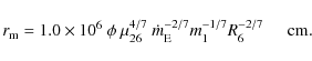
Here
 is the magnetic moment in units of 1026 G cm3, R6 is the NS radius in units of 106 cm,
 the Eddington accretion rate in
  yr-1 (for
R6=1,
yr-1 (for
R6=1,
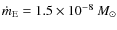 yr-1 and scales with the radius of the compact object), and m1 the NS mass in solar masses.
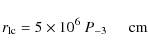
For the radio emission mechanism to switch on in a rotating magnetized
NS, the space surrounding the NS must be free of matter up to the
light cylinder radius (at which the speed of the material co-rotating
with the NS would be equal to the speed of light):
 |
(2) |
where P-3 is the pulse period in milliseconds.
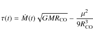
During an outburst, the occurrence, in some cases, of type I bursts
and the observation of coherent X-ray pulsation indicate that at the
origin of the observed luminosity is the accretion mechanism onto the
NS surface. As a consequence coherent radio emission cannot occur in
this phase. In the quiescent state, the 0.5-10 keV luminosity is
detected at levels ranging between 1031.5 and 1034 erg s-1. Accretion of matter at a lower rate was originally proposed to account for this lower luminosity emission. However
detailed studies of the X-ray spectrum in quiescence (Rutledge et al. 2001) and of the thermal relaxation of the NS crust
during this phase (Colpi et al. 2001) suggest that the
cooling of the periodically warmed up NS surface (Brown et al. 1998) is a viable explanation for the bulk of the luminosity in quiescence. If this is the correct interpretation,
there should be no mass accreted onto the neutron star surface
during the X-ray quiescent phase, hence
 ,
and
thus, plausibly,
,
and
thus, plausibly,
 |
(3) |
The timescale for the expansion of the magnetospheric radius beyond the light cylinder radius, in response to a sudden drop in the mass transfer rate, is much shorter (Burderi et al. 2001) than the typical duration (approximately years) of a phase of quiescence in an NS-SXT, allowing the radio pulsar to switch on in principle.
1.1 Absorption effect of the matter surrounding the system
In 2001 Burderi et al. proposed a model able to explain the failure of
previous and subsequent searches (Burgay et al. 2003, and references therein) for pulsed radio emission from quiescent NS-SXTs. As mentioned above, a temporary
significant reduction of the mass-transfer rate may cause the
magnetospheric radius to overcome
 ,
thus allowing a radio
pulsar to switch on. In some cases, even if the secular mass-transfer
rate is restored, the accretion of matter onto the NS can be inhibited
because the radiation pressure from the rotating dipole may be capable of
ejecting most of the matter overflowing from the
companion out of the system. This phase has been defined as radio-ejection. One of
the strongest predictions of this model is the presence, during the
radio-ejection phase (hence during X-ray quiescence), of a strong wind
of matter emanating from the companion star swept away by the
radiation pressure of the pulsar (see Di Salvo et al. 2008a, for a discussion of a possible secular
evolution of these systems). This matter, as well as that residual
from a previous outburst, can play a role in absorbing the radio
signal. Following Burderi et al. (2001) and Burgay et al. (2003), we can estimate the optical depth,
,
thus allowing a radio
pulsar to switch on. In some cases, even if the secular mass-transfer
rate is restored, the accretion of matter onto the NS can be inhibited
because the radiation pressure from the rotating dipole may be capable of
ejecting most of the matter overflowing from the
companion out of the system. This phase has been defined as radio-ejection. One of
the strongest predictions of this model is the presence, during the
radio-ejection phase (hence during X-ray quiescence), of a strong wind
of matter emanating from the companion star swept away by the
radiation pressure of the pulsar (see Di Salvo et al. 2008a, for a discussion of a possible secular
evolution of these systems). This matter, as well as that residual
from a previous outburst, can play a role in absorbing the radio
signal. Following Burderi et al. (2001) and Burgay et al. (2003), we can estimate the optical depth,
 ,
at various radio frequencies due to matter engulfing an NS-SXT in its quiescent phase:
,
at various radio frequencies due to matter engulfing an NS-SXT in its quiescent phase:
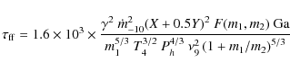
where
 is the mass transfer rate in outburst in units
of
is the mass transfer rate in outburst in units
of
 y-1, X and Y are the mass fraction
of hydrogen and helium respectively,
y-1, X and Y are the mass fraction
of hydrogen and helium respectively,  is the fraction of
ionized hydrogen, T4 the temperature of the outflowing matter in
units of 104 K,
is the fraction of
ionized hydrogen, T4 the temperature of the outflowing matter in
units of 104 K,  the frequency of the radio emission in
units of 109 Hz,
the frequency of the radio emission in
units of 109 Hz,  is the orbital period in hours, m1 and m2 are the masses of the NS and its companion in solar masses,
F(m1, m2) = 1-0.462 m2 / (m1 + m2), Ga = Ga (T4, ,
Z) = 1.00 + 0.48 (
is the orbital period in hours, m1 and m2 are the masses of the NS and its companion in solar masses,
F(m1, m2) = 1-0.462 m2 / (m1 + m2), Ga = Ga (T4, ,
Z) = 1.00 + 0.48 (
 )
- 0.25
)
- 0.25  takes
into account the dependencies of the Gaunt factor from the
temperature, the atomic number Z, and the frequency.
takes
into account the dependencies of the Gaunt factor from the
temperature, the atomic number Z, and the frequency.
One example of a system in the radio-ejection phase is PSR J1740-5340,
an eclipsing MSP, with a spin period of 3.65 ms located in the
globular cluster NGC 6397 (D'Amico et al. 2001). For this source
 at
at  (with X = 0.7, Y = 0.3,
  ,
T4=1,
,
T4=1,
 for Z = 1.1). This shows that the effect of
free-free absorption at 1.4 GHz is important, but not severe, for this
system. The radio signal from this PSR is indeed visible at this
frequency although it is eclipsed and distorted at many orbital phases
(D'Amico et al. 2001). X-ray millisecond pulsars are very similar to PSR J1740-5340, the main difference being the orbital period, which is
for Z = 1.1). This shows that the effect of
free-free absorption at 1.4 GHz is important, but not severe, for this
system. The radio signal from this PSR is indeed visible at this
frequency although it is eclipsed and distorted at many orbital phases
(D'Amico et al. 2001). X-ray millisecond pulsars are very similar to PSR J1740-5340, the main difference being the orbital period, which is  32 h in the case of PSR J1740-5340 and typically ranges from 40 min to 4 h in the case of the X-ray millisecond pulsars. The difference in the orbital period results in a very different optical depth for the free-free absorption caused by the matter present around these systems. But the dependence of
 on the square inverse of the radio frequency implies that, at higher frequencies, the effect of the surrounding matter will be less important. For instance, applying Eq. (4) to one of the tighter orbits AMXPs, XTE J0929-314, at 1.4 GHz, at 6.4 GHz and at 8.5 GHz, with parameters
 ,
,
 ,
,
 ,
X = 0.7, Y = 0.3,
,
X = 0.7, Y = 0.3,
 ,
,
 ,
,
 (Galloway et al. 2002) leads to
(1.4 GHz)
(Galloway et al. 2002) leads to
(1.4 GHz)  5,
(6.5 GHz)
0.2,
(8.5 GHz)
0.1. Adopting these two observing frequencies, the problem of the absorption of the radiation is totally overcome. Prompted by these considerations, we have undertaken a programme to search for millisecond pulsations in NS-SXT XTE J0929-314 at 6.5 and 8.5 GHz.
5,
(6.5 GHz)
0.2,
(8.5 GHz)
0.1. Adopting these two observing frequencies, the problem of the absorption of the radiation is totally overcome. Prompted by these considerations, we have undertaken a programme to search for millisecond pulsations in NS-SXT XTE J0929-314 at 6.5 and 8.5 GHz.
The observations and the method of data analysis are presented in Sect. 2, and the results are reported in Sect. 3 and discussed in Sect. 4.
2 Observations and data analysis
Radio observations of the millisecond pulsar XTE J0929-314 were made with the Parkes 64 m radio telescope. Three data series were taken on 2003 December 19-21 with a bandwidth of 576 MHz. The first was at a central radio frequency of 6410.5 MHz, the other two at a central radio frequency of 8453.5 MHz.
The collected signal for each polarization was split into 192 3 MHz
channels using an analogue filterbank, in order to minimize the pulse
broadening caused by dispersion in the interstellar medium (ISM). The
outputs from each channel were one bit digitized every 100 s.
The resulting time series were stored on digital linear tapes (DLT)
for off-line analysis. The observations lasted 7.5 h each,
corresponding to 228 samples. We then rebinned the data to obtain
227 samples in order to reduce the computational time; therefore,
the effective time resolution of the analysed data is 200 s.
The data analysis methodology was chosen on the basis of the precise knowledge of the orbital and spin parameters for XTE J0929-314, obtained from the X observation. The original ephemerides were presented by Galloway et al. (2002), while we used those reported in Table 1, which have been recently refined by Di Salvo et al. (in prep.; see also Di Salvo et al. 2008b).
Off-line analysis was made by means of a software suite that, in the
first stage, aimed to reduce the dispersion effects on the signal due
to the interstellar medium. The data series were dedispersed according
to 72 trial dispersion-measure (DM) values ranging from 5.51 to 396.74 pc cm-3 for the data series at 6410.5 MHz and 33 trial DM values ranging from 12.64 to 416.99 pc cm-3 for the data
series at 8453.5 MHz. The maximum DM was chosen to be 4 times the nominal DM value obtained using either the Taylor & Cordes (1993) or the Cordes & Lazio (2001) models for the distribution of free electrons in the ISM, in order to account
for the errors in the estimated distance of the source, for the uncertainties in the ISM model, and for the presence of local matter surrounding the system, hence increasing the
local DM (estimated to be at most 100 pc/cm3 for this source; Burgay et al. 2003).
The successive step is to deorbit and barycentre the time series, i.e. to eliminate the effects of the orbital motion of the NS in the binary system and the earth in the solar system. This was obtained by resampling the time series in order to mimick time series collected from a telescope located in the barycentre of the solar system and looking at the source as if it were located at the barycentre of the pulsar orbit.
Table 1: Orbital and spin parameters for XTE J0929-314 (Di Salvo et al., in prep.; see also Di Salvo et al. 2008b).
In doing this exercise it is important to estimate the effect on the
putative pulsar signal due to the uncertainties in the adopted
ephemeris for the system. Therefore we simulated dedispersed time
series containing a periodic signal with the spin and orbital
characteristics of XTE J0929-314, as derived by Di Salvo et al. (Table 1). We then deorbited and barycentred these time series using the upper and the lower limits of the parameters in Table 1, adopting 1 errors.
It turned out that even a variation in all the parameters (but the orbital period, see later) at  level does not affect the detectability of the pulsations, since that produced a maximum
broadening of the pulse much smaller than 0.1 in pulsar phase. The only exception is for the orbital period: 1
variation in
level does not affect the detectability of the pulsations, since that produced a maximum
broadening of the pulse much smaller than 0.1 in pulsar phase. The only exception is for the orbital period: 1
variation in
 ,
propagated over the 19 500 orbits occurred between X-ray and radio observations, produces a broadening of 0.4 in pulsar phase for our observation. Therefore, to obtain a maximum broadening of the pulse of 0.1 in phase, we corrected the time series using 8 trial values of
(4 above and 4 below the
nominal value), covering the 1
uncertainty range.
,
propagated over the 19 500 orbits occurred between X-ray and radio observations, produces a broadening of 0.4 in pulsar phase for our observation. Therefore, to obtain a maximum broadening of the pulse of 0.1 in phase, we corrected the time series using 8 trial values of
(4 above and 4 below the
nominal value), covering the 1
uncertainty range.
The third step in the procedure was to fold the (already deorbited and
barycentred) time series according to the rotational parameters
reported in Table 1. The trial values of the spin
period used for the folding, were chosen taking into account that
the nominal value of  dates from the X-ray observations of May
2002, while our observations occurred 19 months later. Therefore we
explored a range of spin period
dates from the X-ray observations of May
2002, while our observations occurred 19 months later. Therefore we
explored a range of spin period
 ,
with
,
with
 and
and
 ,
where
and
,
where
and  are the values reported in Table 1,
 and
and
 their 1
errors, and
their 1
errors, and  T is the time between the observations in X-ray and radio bands. As a first guess we used the outburst value of
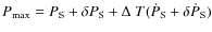
 for this calculation, resulting a safe upper limit for the dipolar spin-down
![]() , as shown below. For a safer investigation, we also checked on spin period values lower than our previous estimate
, as shown below. For a safer investigation, we also checked on spin period values lower than our previous estimate
 and for the double of the nominal value,
 .
.
Since the spin period derivative measured in outburst is usually
different from that in the quiescent phase, we checked the
plausibility of the adopted trial period interval through an estimate
of the surface magnetic field  .
This estimate can be obtained
evaluating the magnetic torque acting on the NS through the formula
(Rappaport et al. 2004; Di Salvo et al., in prep.):
.
This estimate can be obtained
evaluating the magnetic torque acting on the NS through the formula
(Rappaport et al. 2004; Di Salvo et al., in prep.):
where
 is the mass accretion rate, M the NS mass, the magnetic dipole moment,
 the corotation radius (at
which the disc matter in Keplerian motion rotates with the same
angular speed of the NS) in cgs units. Since this AMXP is observed to
spin down, the contribution to the spin up from the accretion (first
additive term in 5) is neglected. The torque can also
be written:
the corotation radius (at
which the disc matter in Keplerian motion rotates with the same
angular speed of the NS) in cgs units. Since this AMXP is observed to
spin down, the contribution to the spin up from the accretion (first
additive term in 5) is neglected. The torque can also
be written:
 |
(6) |
where I is the NS moment of inertia and
 the spin
frequency derivative. Since
and
are known and,
assuming
I = 1045 g cm2, we can obtain the value of the
magnetic moment and, in turn, an estimate of .
Then, through the relation
the spin
frequency derivative. Since
and
are known and,
assuming
I = 1045 g cm2, we can obtain the value of the
magnetic moment and, in turn, an estimate of .
Then, through the relation
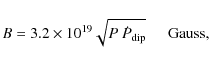 |
(7) |
we can obtain an estimate of the dipolar spin-down
 during observation (in quiescence),
assuming the spin down is governed by magnetodipole braking. It
leads to
during observation (in quiescence),
assuming the spin down is governed by magnetodipole braking. It
leads to
 Gauss and
 and then we can conclude that the adopted
 is safely large.
Therefore, since the pulse broadening for an error equal to 1/20 of the
is safely large.
Therefore, since the pulse broadening for an error equal to 1/20 of the  interval is less than 0.1 in phase over our observations, we selected 40 trial values of the period, 20 to the right and 20 to the left of the nominal value to cover the
interval calculated above.
interval is less than 0.1 in phase over our observations, we selected 40 trial values of the period, 20 to the right and 20 to the left of the nominal value to cover the
interval calculated above.
A further check of the validity of the derived
(hence of the adopted
)
can be derived from optical observations (Monelli et al. 2005; D'Avanzo et al. 2008). In fact, the optical counterpart of the XTE J0929-314 companion observed in December 2003 (very close to our radio observations) with the VLT has a luminosity one order of magnitude higher than expected. This luminosity excess can be interpreted as the luminosity
 isotropically irradiated by the rotating magneto-dipole, intercepted, and reprocessed by the companion star, as observed e.g. by Burderi et al. (2003) and Campana et al. (2004) for SAX J1808.4-3658, and by D'Avanzo et al. (2007) for IGR J00291+5934.
The excess luminosity can be written as the fraction
 of dipolar radiation intercepted by the companion star and the disk (see Burderi et al. 2003):
 |
(8) |
where
 is the rotational frequency of the NS and
  can be written as
 )/(4
)/(4 a2), where a is the the orbital separation and
  the angle subtended by the companion star as seen from the central source. If the companion star fills its Roche lobe, this can be written as
 ,
where
,
where
 is the Roche lobe radius of the secondary and
 /[0.6
/[0.6
 )] (Eggleton 1983). Assuming a mass ratio of
q = m2/m2=0.02/1.4 and
)] (Eggleton 1983). Assuming a mass ratio of
q = m2/m2=0.02/1.4 and
 ,
we obtain
,
we obtain
 ;
while
;
while
 is evaluated adopting a standard Shakura-Sunyaev disk model (Shakura & Sunyaev 1973) with
 ,
and is given by the projected area of the disk as seen by the central source, 2
,
and is given by the projected area of the disk as seen by the central source, 2
 (where R is the disk outer radius and H(R) the disk semi-thickness at R), divided by the total area, 4
 .
.
Adopting the value of
 erg s-1 reported by Monelli et al. (2005) and
 ,
we can thus derive
,
we can thus derive
 Gauss, in good agreement with the value estimated above.
3 Results
Spanning the searched ranges of
,
and DM we have
obtained 50 922 plots, reporting the result from the folding of the
deorbited and barycentred time series.
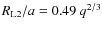
An example of these plots (obtained from the observation at 6.5 GHz) is shown in
Fig. 1. The bottom diagram shows the integrated
pulse profile (6 phases), while the grayscale on the left represents
the signal in the 255 subintegrations in which the observation has
been subdivided. A good candidate should display a roughly linear
trend in the grayscale and a high signal-to-noise ratio pulse
profile. On the right, the parameters used for the folding of this
candidate are shown, along with the parameters of the observation.
![\begin{figure}
\par\includegraphics[width=8.8cm,clip]{0677fig1.eps}
\end{figure}](/articles/aa/full_html/2009/14/aa10677-08/img93.png) |
Figure 1: Example of a plot resulting from the procedure described in the text. The bottom diagram shows six integrated pulse profiles, while the grayscale on the left represents the signal in the 255 subintegrations in which the observation has been subdivided. On the right, the parameters used for the folding are shown, along with the parameters of the observation. |
| Open with DEXTER | |
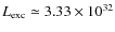
A useful diagnostic tool that can be adopted to further evaluate the
plausibility of a suspect is shown in Fig. 2, where a
grayscale of the strength of the signal (with darker points at
higher S/N), plotted as a function of dispersion measure DM and spin frequency
 ,
should define a clear peak around the correct parameters of the
putative pulsar. The same kind of plot can be created at a constant DM
with
and
on the axes or at a constant
,
tracing the S/N trend at varying DMs and
s.
,
should define a clear peak around the correct parameters of the
putative pulsar. The same kind of plot can be created at a constant DM
with
and
on the axes or at a constant
,
tracing the S/N trend at varying DMs and
s.
The plots in Figs. 1 and 2 refer to the suspect with the highest S/N found in our search. Its folding parameters are listed in Table 2. The peak in the profile has a 3.4
significance that, over the 26 568 trial foldings performed on the 6.5 GHz dataset (72 DMs  9
s
41 s), has a probability of not being randomly generated by noise of 10-6. We also note that, in Fig. 2 the decreasing S/N trend is not particularly defined, although a maximum is present. Also, that the DM that maximises the S/N is close to zero (w.r.t an expected value of
9
s
41 s), has a probability of not being randomly generated by noise of 10-6. We also note that, in Fig. 2 the decreasing S/N trend is not particularly defined, although a maximum is present. Also, that the DM that maximises the S/N is close to zero (w.r.t an expected value of
 100 pc/cm3) weakens the credibility of the signal. Finally, this signal suspect is
not confirmed in the observations at higher frequency (8.5 GHz), elaborated with the same parameters.
We can conclude that no radio pulsation with the expected
periodicity has been found in the source XTE J0929-314 during its
quiescent phase.
100 pc/cm3) weakens the credibility of the signal. Finally, this signal suspect is
not confirmed in the observations at higher frequency (8.5 GHz), elaborated with the same parameters.
We can conclude that no radio pulsation with the expected
periodicity has been found in the source XTE J0929-314 during its
quiescent phase.
Table 2: Parameters for the pulsar candidate with the highest S/N shown in Fig. 1.
![\begin{figure}
\par\includegraphics[width=5.6cm,angle=-90,clip]{0677fig2.epsi}
\end{figure}](/articles/aa/full_html/2009/14/aa10677-08/img98.png) |
Figure 2:
Signal-to-noise ratio in function of the spin frequency (20 step above and 20 below the nominal value, corresponding to 0) and the dispersion measure (72 steps corresponding to values interval from 5.51 to 396.74 cm-3 pc) at
|
| Open with DEXTER | |
 s.
The highest point corresponds to the best S/N,
s.
The highest point corresponds to the best S/N,
3.1 Flux density upper limits
A rough estimate of the flux density for a pulsar of period P is (e.g. Manchester et al. 1996)
where
 is the threshold (in unit of sigma) for having a statistically significant signal, given the number of performed foldings;
 K the system noise temperature for the observations at 6 GHz and
 K for those at 8 GHz (see Parkes website: http://www.parkes.atnf.csiro.au/observing/documentation);
 is the sky temperature in Kelvin, calculated from that at
 MHz and considering a scaling with the frequency as
 ;
G is the gain of the radio telescope (in K Jy-1), with 0.46 for the observations at 6 GHz and 0.59 for those at 8 GHz, (see Parkes website);
;
G is the gain of the radio telescope (in K Jy-1), with 0.46 for the observations at 6 GHz and 0.59 for those at 8 GHz, (see Parkes website);  is the integration time in seconds,
  the number of polarizations (here 2), and
 MHz is the bandwidth in MHz. The term
 is a factor accounting for the sensitivity reduction due to digitisation and other losses. The term
  is the effective width of the pulse:

Its value depends on the sampling time (
 s in this
case), on the technical characteristics of the receiver (
s in this
case), on the technical characteristics of the receiver ( ),
on the broadening of the pulse introduced by both the dispersion of
the signal in each channel (
),
on the broadening of the pulse introduced by both the dispersion of
the signal in each channel (
 DM s, depending on the frequency), on the scattering
induced by inhomogeneities in the ISM (
DM s, depending on the frequency), on the scattering
induced by inhomogeneities in the ISM (
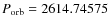
 s), and on the intrinsic pulse width W. The dependence of the minimum flux density achievable from the duty cycle, W/P, is shown in Fig. 3. A duty cycle of 15% of the spin period is assumed and, with this
value, the flux density upper limits for XTE J0929-314 are:
s), and on the intrinsic pulse width W. The dependence of the minimum flux density achievable from the duty cycle, W/P, is shown in Fig. 3. A duty cycle of 15% of the spin period is assumed and, with this
value, the flux density upper limits for XTE J0929-314 are:
 Jy at 6410.5 MHz and
 Jy at 8453.5 MHz.
![\begin{figure}
\par\includegraphics[width=8.8cm,clip]{0677fig3.eps}
\end{figure}](/articles/aa/full_html/2009/14/aa10677-08/img118.png) |
Figure 3:
Flux density upper limits in |
| Open with DEXTER | |
4 Discussion
In the hypothesis that a radio pulsar was on during our observations, we examine several possible explanations for the lack of the detection of radio pulsation from our source.
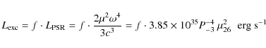
4.1 The luminosity
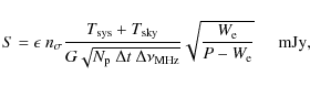
In Fig. 4 the pseudoluminosity
 in
mJy kpc2 (where S is the measured flux density and d the
distance of the source) distribution at 1.4 GHz for a sample of 42
galactic field MSPs is shown
in
mJy kpc2 (where S is the measured flux density and d the
distance of the source) distribution at 1.4 GHz for a sample of 42
galactic field MSPs is shown![]() .
For XTE J0929-314 the upper limits on the pseudoluminosity has been calculated assuming a distance of 6 kpc (Galloway et al. 2002) and our flux density upper limits at 6.4 and 8.5 GHz scaled to 1.4 GHz assuming a spectral index for MSPs of 1.7 (Kramer et al. 1998). As a result, about 90% of the known MSPs are below the pseudoluminosity upper limits of XTE J0929-314.
.
For XTE J0929-314 the upper limits on the pseudoluminosity has been calculated assuming a distance of 6 kpc (Galloway et al. 2002) and our flux density upper limits at 6.4 and 8.5 GHz scaled to 1.4 GHz assuming a spectral index for MSPs of 1.7 (Kramer et al. 1998). As a result, about 90% of the known MSPs are below the pseudoluminosity upper limits of XTE J0929-314.
![\begin{figure}
\par\includegraphics[width=9cm]{0677fig4.eps}
\end{figure}](/articles/aa/full_html/2009/14/aa10677-08/img120.png) |
Figure 4: Pseudoluminosity distribution of a sample of 42 field MSPs. The arrows indicate the upper limits of the pseudoluminosity scaled at 1.4 GHz for XTE J0929-314, derived on the basis of the minimum flux detectable and assuming a distance of 6 kpc (Galloway et al. 2002). |
| Open with DEXTER | |
This suggests that XTE J0929-314 in quiescence might not be a very bright MSP and that a deeper search should be carried out to sample lower values of the flux density. However, given the distance of XTE J0929-314 (significantly higher than the typical distance of the sample of known MSPs), only next-generation instruments, like the Square Kilometer Array, will be able to discover pulsed radio emission from this source at the high frequencies adopted in this work, if its luminosity is at the faintest end of the known distribution.
4.2 The beaming factor
The emission from a pulsar is strongly anisotropic. This means that it does not irradiate in the same way in all directions, but only on one usually narrow portion of sky, which can be quantified through the so-called beaming factor. Therefore, the lack of a detection of a radio signal could be due to unfavourable geometry of the radio emission with respect to the observer.
The average value,  ,
of the fraction of the sky swept from
two conal radio beams of half width
,
of the fraction of the sky swept from
two conal radio beams of half width  is (Emmering & Chevalier
1989):
is (Emmering & Chevalier
1989):

where
 is the angle (supposed randomly distributed) between the
magnetic axis (aligned with the radio beams) and the rotational axis,
and
is the angle (supposed randomly distributed) between the
magnetic axis (aligned with the radio beams) and the rotational axis,
and
![$f(\alpha,\eta)=\cos[\max(0,~ \eta-\alpha)]-\cos[\min(0,~ \eta+\alpha )]$](/articles/aa/full_html/2009/14/aa10677-08/img125.png) .
.
Considering a 10%  30% interval of width of the pulse, it
follows that
30% interval of width of the pulse, it
follows that
 and, therefore, using
Eq. (11),
and, therefore, using
Eq. (11),
 . In particular,
assuming 15% typical value of width of the impulse, the probability
that the radio emission cone does not intersect our line of sight is
66%, with
. In particular,
assuming 15% typical value of width of the impulse, the probability
that the radio emission cone does not intersect our line of sight is
66%, with
 .
.
5 Conclusions
The aim of this work was to search for radio pulsations from the AMXP
XTE J0929-314. The detection of radio signals in the quiescent phase
of this kind of transient systems would be ultimate proof of the
recycling model, unambiguously establishing that the AMXPs are the
progenitors of radio MSP. No radio pulsation has been detected in the
analysed data down to a limit of 68 Jy at 6.4 GHz and 26 Jy
at 8.5 GHz. Assuming that a radio pulsar was on during the observation,
the free-free absorption cannot be responsible for the lack of a
detection, given the relatively high radio frequencies. The
beaming factor is a viable explanation for that, since the probability
of any unfavourable geometry of radio emission with respect to the
observer is
 .
However, the most likely reason for a
negative result is that the source has a luminosity lower than our
limits. In fact, more than 90% of the known MSPs show a luminosity
lower than the upper limits that we have derived for XTE J0929-314.
.
However, the most likely reason for a
negative result is that the source has a luminosity lower than our
limits. In fact, more than 90% of the known MSPs show a luminosity
lower than the upper limits that we have derived for XTE J0929-314.
To get round to these problems, one can make observations at an intermediate frequency between 6.5 and 1.4 GHz. For a maximum mass transfer rate in quiescence equal to the outburst value, we can estimate that the lower limit in frequency for obtaining
 is 3 GHz. Calculating
 for an observation with all the same parameters (adopted in the present work) but the frequency (now set at 3 GHz), we could sample more than a half of the known MSPs luminosity distribution.
Acknowledgements
A.P. and M.B. acknowledge the financial support to this research provided by the Ministero dell'Istruzione, dell'Università e della Ricerca (MIUR) under the national programme PRIN052005024090_002.
References
- natexlab
- Alpar, M. A., Cheng, A. F., Ruderman, M. A., & Shaham, J. 1982, Nature, 300, 728 In the text
- Altamirano, D., Casella, P., Patruno, A., Wijnands, R., & van der Klis, M. 2008, ApJ, 674, L45 In the text
- Bhattacharya, D., & van den Heuvel, E. P. J. 1991, Phys. Rep., 203, 1 In the text
- Brown, E. F., Bildsten, L., & Rutledge, R. E. 1998, ApJ, 504, L95 In the text
- Burderi, L., Possenti, A., D'Antona, F., et al. 2001, ApJ, 560, L71 In the text
- Burderi, L., Di Salvo, T., D'Antona, F., Robba, N. R., & Testa, V. 2003, A&A, 404, L43 In the text
- Burgay, M., Burderi, L., Possenti, A., et al. 2003, ApJ, 589, 902 In the text
- Campana, S., Colpi, M., Mereghetti, S., Stella, L., & Tavani, M. 1998, A&ARv, 8, 279 In the text
- Casella, P., Altamirano, D., Patruno, A., Wijnands, R., & van der Klis, M. 2008, ApJ, 674, L41 In the text
- Chakrabarty, D., & H., M. E. 1998, Nature, 394, 346 In the text
- Colpi, M., Geppert, U., Page, D., & Possenti, A. 2001, ApJ, 548, L175 In the text
- Cordes, J. M., & Lazio, T. J. W. 2001, ApJ, 549, 997 In the text
- D'Amico, N., Possenti, A., Manchester, R. N., et al. 2001, ApJ, 561, L89
- D'Avanzo, P., Campana, S., Casares, J., et al. 2008, AIP Conf. Ser., 1068, 217
- Di Salvo, T., Burderi, L., Riggio, A., Papitto, A., & Menna, M. T. 2008a, MNRAS, 389, 1851 In the text
- Di Salvo, T., Burderi, L., Riggio, A., Papitto, A., & Menna, M. T. 2008b, AIP Conf. Ser., 1054, 173 In the text
- Eggleton, P. P. 1983, ApJ, 268, 368 In the text
- Emmering, R. T., & Chevalier, R. A. 1989, ApJ, 345, 931 In the text
- Galloway, D. K., Chakrabarty, D., Morgan, E. H., & Remillard, R. A. 2002, ApJ, 576, L137 In the text
- Kramer, M., Xilouris, K. M., Lorimer, D. R., et al. 1998, ApJ, 501, 270 In the text
- Krimm, H. A., Markwardt, C. B., Deloye, C. J., et al. 2007, ApJ, 668, L147 In the text
- Manchester, R. N., Lyne, A. G., D'Amico, N., et al. 1996, MNRAS, 279, 1235 In the text
- Manchester, R. N., Hobbs, G. B., Teoh, A., & Hobbs, M. 2005, VizieR Online Data Catalog, 7245, 0
- Monelli, M., Fiorentino, G., Burderi, L., et al. 2005, in Interacting Binaries: Accretion, Evolution, and Outcomes, ed. L. Burderi, L. A. Antonelli, F. D'Antona, et al., AIP Conf. Ser., 797, 565 In the text
- Rappaport, S. A., Fregeau, J. M., & Spruit, H. 2004, ApJ, 606, 436 In the text
- Rutledge, R. E., Bildsten, L., Brown, E. F., Pavlov, G. G., & Zavlin, V. E. 2001, ApJ, 559, 1054 In the text
- Shakura, N. I., & Syunyaev, R. A. 1973, A&A, 24, 337 In the text
- Taylor, J. H., & Cordes, J. M. 1993, ApJ, 411, 674 In the text
- White, N. E., Nagase, F., & Parmar, A. N. 1995, in X-ray binaries, ed. W. H. G. Lewin, J. van Paradijs, & E. P. J. van den Heuvel (Cambridge University Press), 1 In the text
- Wijnands, R. 2006, in BAAS, 38, 1183 In the text
- Wijnands, R., & van der Klis, M. 1998, Nature, 394, 344 In the text
Footnotes
- ... spin-down
![[*]](/icons/foot_motif.png)
- The expected variation of the
during the radio observation is negligible and hence does not affect a correct folding.
- ... shown
- These values are derived from the ATNF catalogue - http://www.atnf.csiro.au/research/pulsar/psrcat/; Manchester et al. (2005).
All Tables
Table 1: Orbital and spin parameters for XTE J0929-314 (Di Salvo et al., in prep.; see also Di Salvo et al. 2008b).
Table 2: Parameters for the pulsar candidate with the highest S/N shown in Fig. 1.
All Figures
| |
Figure 1: Example of a plot resulting from the procedure described in the text. The bottom diagram shows six integrated pulse profiles, while the grayscale on the left represents the signal in the 255 subintegrations in which the observation has been subdivided. On the right, the parameters used for the folding are shown, along with the parameters of the observation. |
| Open with DEXTER | |
| In the text | |
| |
Figure 2:
Signal-to-noise ratio in function of the spin frequency (20 step above and 20 below the nominal value, corresponding to 0) and the dispersion measure (72 steps corresponding to values interval from 5.51 to 396.74 cm-3 pc) at
|
| Open with DEXTER | |
| In the text | |
| |
Figure 3:
Flux density upper limits in |
| Open with DEXTER | |
| In the text | |
| |
Figure 4: Pseudoluminosity distribution of a sample of 42 field MSPs. The arrows indicate the upper limits of the pseudoluminosity scaled at 1.4 GHz for XTE J0929-314, derived on the basis of the minimum flux detectable and assuming a distance of 6 kpc (Galloway et al. 2002). |
| Open with DEXTER | |
| In the text | |
Copyright ESO 2009
Current usage metrics show cumulative count of Article Views (full-text article views including HTML views, PDF and ePub downloads, according to the available data) and Abstracts Views on Vision4Press platform.
Data correspond to usage on the plateform after 2015. The current usage metrics is available 48-96 hours after online publication and is updated daily on week days.
Initial download of the metrics may take a while.