| Issue |
A&A
Volume 496, Number 3, March IV 2009
|
|
|---|---|---|
| Page(s) | 869 - 877 | |
| Section | Planets and planetary systems | |
| DOI | https://doi.org/10.1051/0004-6361/200810509 | |
| Published online | 30 January 2009 | |
Consequences of expanding exoplanetary atmospheres for magnetospheres
E. P. G. Johansson1 - T. Bagdonat1 - U. Motschmann1,2
1 -
Institute for Theoretical Physics, TU Braunschweig,
Mendelssohnstrasse 3, 38106 Braunschweig, Germany
2 -
Institute for Planetary Research, DLR, Berlin, Germany
Received 3 July 2008 / Accepted 5 January 2009
Abstract
The atmospheres of close-in extrasolar planets are expected to both undergo hydrodynamic expansion due to strong heating and produce strong expanding ionospheres due to intense photoionization, while at the same time being exposed to strong stellar winds. This scenario can be expected to lead to new types of magnetospheres and previously unseen interactions between stellar wind plasma and ionospheres. Our aim is to start looking at these kinds of scenarios for close-in terrestrial planets using hybrid simulations.
For this purpose we used a hybrid code, treating electrons as a massless, charge-neutralizing, adiabatic fluid and ions as macroparticles, to study the influence of a strongly expanding ionosphere on the stellar wind interaction for an unmagnetized close-in extrasolar terrestrial planet.
For both with and without expansion, we can identify bow shock, magnetopause, and ion-composition boundary. The expanding ionosphere pushes the bow shock, magnetic draping, and ion composition boundary upstream and increases the size of the entire interaction region, creating a large wake behind the planet, largely void of electromagnetic fields and dominated only by the expanding ionosphere. On the dayside, little ionospheric radial bulk flow is actually observed since the ions are quickly thermalized after being added to the ionosphere.
Key words: plasmas - stars: planetary systems - stars: winds, outflows - magnetic fields
1 Introduction
Of the ![]() 304 extrasolar planets
304 extrasolar planets![]() discovered to date, a substantial fraction (
discovered to date, a substantial fraction (![]() 90 exoplanets or
90 exoplanets or ![]() )
are so called close-in extrasolar giant planets, orbiting at close ranges of
)
are so called close-in extrasolar giant planets, orbiting at close ranges of
![]() .
New research programs, like the now ongoing Convection Rotation and planetary Transits (CoRoT) mission and the future Kepler Mission will within the foreseeable future detect and investigate not only close-in giant planets but also close-in terrestrial planets (Bordé et al. 2003; Marcy et al. 2006). The domination of giants planets among the already known close-in extrasolar planets is very likely an observational effect and we speculate, based on theory and simulations of planet formation as well as the statistics of known exoplanets (Lin 2006; Raymond et al. 2006; Lovis et al. 2006), that there is also a significant population of close-in terrestrial planets, yet to be discovered.
.
New research programs, like the now ongoing Convection Rotation and planetary Transits (CoRoT) mission and the future Kepler Mission will within the foreseeable future detect and investigate not only close-in giant planets but also close-in terrestrial planets (Bordé et al. 2003; Marcy et al. 2006). The domination of giants planets among the already known close-in extrasolar planets is very likely an observational effect and we speculate, based on theory and simulations of planet formation as well as the statistics of known exoplanets (Lin 2006; Raymond et al. 2006; Lovis et al. 2006), that there is also a significant population of close-in terrestrial planets, yet to be discovered.
Due to the proximity to their respective host stars one can expect close-in exoplanets to be exposed to very different stellar winds and plasma environments compared to the familiar bodies of the solar system, but whereas the solar wind interactions with various solar system bodies have for long been studied, not much is known about the equivalent extrasolar stellar wind interactions with close-in extrasolar planets.
The stellar wind interactions in these close-in orbits can be expected to be different for multiple reasons and there are several expected scenarios that may take place: 1) the close-in stellar wind is different from farther out, e.g. slower, hotter, denser and with a stronger frozen-in magnetic field and may lead to subsonic flows sufficiently close to the host star (Preusse et al. 2005; Ip et al. 2004) as opposed to in most of the solar system; 2) the high orbital velocities paired with the Parker spiral geometry of the interplanetary magnetic field leads to a range of orbits with quasiparallel interaction, i.e. the interplanetary magnetic field being approximately parallel to the direction of the stellar wind in the frame of the exoplanet; 3) strong tidal interactions with the star may slow down or even halt planetary rotation. Absence of planetary rotation in turn completely or mostly eliminates any internal dynamo and therefor intrinsic magnetic field, thus leaving the planet's atmosphere and ionosphere unprotected from the stellar wind (Griessmeier et al. 2004), similar to the situation for Venus; 4) the proximity to the star implies intense photoionization and thus stronger ionosphere, free to interact with the stellar wind; 5) intense dayside heating leading to hydrodynamically expanding as well as strongly expanded atmospheres up to altitudes of planetary radii (Vidal-Madjar et al. 2004; Yelle 2004; Tian et al. 2005; Lammer et al. 2004; Vidal-Madjar et al. 2003). All these scenarios speak for that we should expect very different and unexplored stellar wind interactions.
The now famous observations of transiting close-in extrasolar giant planet HD 209458 b (Vidal-Madjar et al. 2004,2003) seem to imply that the planet possesses an extended and constantly expanding atmosphere, reaching altitudes of several planetary radii and thus fitting the last category above. A great number of articles have followed trying to find out what such an atmosphere may look like, which mechanisms that can generate such an expansion and what kinds of mass loss rates one can expect as well as its subsequent implications for planetary evolution (Lammer et al. 2003,2004; Lecavelier des Etangs et al. 2004; Yelle 2004; Tian et al. 2005; Baraffe et al. 2004; Hubbard et al. 2007; Holmström et al. 2008). In principle, this should not be an unusual scenario, given that there are many close-in extrasolar planets exposed to similar conditions.
We are especially interested in the terrestrial counterparts to the above scenario. Therefore the aim of this article is to start looking at similar scenarios via simulations of the stellar wind interaction with the expanding ionosphere which should accompany the expanding atmosphere of a close-in extrasolar terrestrial planet. We do this with a hybrid code since it, as opposed to pure fluid approaches like magnetohydrodynamics (MHD), also can handle non-Maxwellian velocity distributions and resolve kinetic effects in regions with sufficiently low magnetic field strength, like the tail region in our simulation results, but also because we have a well tested hybrid code, ``the Braunschweig code'', available locally.
Stellar wind interaction with extrasolar planets has been simulated before by among others Ip et al. (2004, MHD), Lipatov et al. (2005, both hybrid simulation and drift-kinetic) and Preusse et al. (2007, MHD).
2 Model description
2.1 Code description
The plasma simulation code used, ``The Braunschweig code'', was introduced in Bagdonat & Motschmann (2002) to simulate the solar wind interaction with comets, but has since then been modified to simulate the solar wind interaction for extended celestial bodies, like Mars and Titan (see e.g. Simon et al. 2006; Boesswetter et al. 2007,2004). The basic premise for the simulations is an obstacle, e.g. a planet with an ionospheric plasma, located at the center of a three-dimensional simulation box which is then immersed in a stellar wind plasma flow and time integrated until reaching a quasistationary state. The time integration scheme is based on that introduced by Matthews (1994).
The Braunschweig code is a hybrid code, meaning that it represents plasmas by simultaneously using a macroparticle description for the ions and a massless fluid description for the electrons. The macroparticles, each representing a larger number of physical ions, move solely under the influence of the Lorentz force, a drag force due to collisions with a prescribed neutral background atmosphere, and a planetary gravity field according to
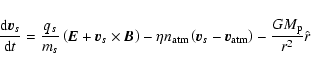
where vs, qs and ms are the velocity, charge and mass of a particular macroparticle of ion species s.
We use the assumption of an electron fluid with a momentum equation
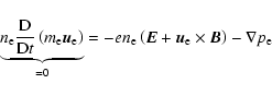
where
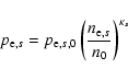
An actual electron fluid may consist of several components of different origin and different thermal properties which would require multiple versions of the electron fluid momentum Eq. (2) and additional coupling equations. Since this would complicate the time integration, we use a somewhat simpler model where the total electron fluid pressure ![]() is the sum of the contributions
is the sum of the contributions
![]() from one adiabatic electron fluid per ion species s
from one adiabatic electron fluid per ion species s
 |
(3) |
where
We also assume quasineutrality within every ion species, i.e.
| (4) |
where
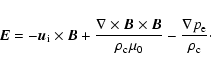
Using the aforementioned assumptions together with Faraday's law and the Darwin approximation
| (5) |
i.e. Ampère's law with
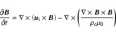
where
The ion number density
The planet itself is implemented as a spherical region in the simulation box with an imposed constant density and zero ion velocity. All macroparticles that enter it are removed. The planetary ionosphere is implemented as a continuosly plasma producing region surrounding the planet. No recombination process is implemented. The simulation box boundaries are all inflow boundaries, i.e. with imposed field and plasma values, except the downstream boundary (positive x boundary) which is an outflow boundary, i.e. plasma is removed and field values are copied from those in adjacent cells inside the simulation box.
2.2 Model parameters
Our scenario is in several aspects chosen to approximate that of an Earth-like body orbiting a Sun-like star at an orbital distance of
![]() .
Thus we use a planetary mass of
.
Thus we use a planetary mass of
![]() and a planetary radius of
and a planetary radius of
![]() .
Our planet does however not have an intrinsic magnetic field.
.
Our planet does however not have an intrinsic magnetic field.
The size of our simulation box is
![]() and it is divided into
and it is divided into
![]() approximately cube-shaped cells. The planet is located
approximately cube-shaped cells. The planet is located
![]() downstream of the center of the simulation box. We also use two different ion species: one hydrogen species for the stellar wind and one hydrogen species for the ionospheric plasma. There are three reasons for numerically using two different hydrogen ion species: 1) to let us follow the plasmas of different origin; 2) to enable the code's use of different electron temperatures for stellar wind and ionospheric plasma; and 3) to enable the code's macroparticles to represent different numbers of physical ions for the different plasmas, which in turn saves memory and computations.
downstream of the center of the simulation box. We also use two different ion species: one hydrogen species for the stellar wind and one hydrogen species for the ionospheric plasma. There are three reasons for numerically using two different hydrogen ion species: 1) to let us follow the plasmas of different origin; 2) to enable the code's use of different electron temperatures for stellar wind and ionospheric plasma; and 3) to enable the code's macroparticles to represent different numbers of physical ions for the different plasmas, which in turn saves memory and computations.
All simulations have been running for a time equivalent to an undisturbed stellar wind passing through the box more than seven times, at which point they have all reached a quasistationary state.
2.2.1 Stellar wind parameters
By using a Parker stellar wind model (Parker 1958) and fitting it to the Sun and the solar wind speed
![]() at
at
![]() (Schwenn 1990) it is possible to calculate an approximate stellar wind speed of
(Schwenn 1990) it is possible to calculate an approximate stellar wind speed of
![]() in a non-orbiting frame at
in a non-orbiting frame at
![]() .
At these small orbital distances it starts to become important to distinguish between absolute and relative stellar wind speed since the orbital velocity becomes comparable to the stellar wind speed. For the same reason, the stellar wind direction will appear to be different in that frame, thus changing the angle between the stellar wind velocity and the magnetic field (Zarka et al. 2001).
.
At these small orbital distances it starts to become important to distinguish between absolute and relative stellar wind speed since the orbital velocity becomes comparable to the stellar wind speed. For the same reason, the stellar wind direction will appear to be different in that frame, thus changing the angle between the stellar wind velocity and the magnetic field (Zarka et al. 2001).
Accounting for this orbital motion by assuming a stellar mass of
![]() and rounding off gives us a stellar wind speed in the frame of the planet of
and rounding off gives us a stellar wind speed in the frame of the planet of
![]() .
Using the estimated solar wind mass loss rate in Mann et al. (1999) and assuming spherical symmetry together with a stellar wind as above gives us a stellar wind number density of
.
Using the estimated solar wind mass loss rate in Mann et al. (1999) and assuming spherical symmetry together with a stellar wind as above gives us a stellar wind number density of
![]() at
at
![]() .
The frozen-in magnetic field (interplanetary magnetic field, IMF) used is
.
The frozen-in magnetic field (interplanetary magnetic field, IMF) used is
![]() .
.
The stellar wind temperatures are based on a scaling law for the solar wind used in Schwenn & Marsch (1991),
 |
(8) |
where
The above given values correspond to an Alfvénic Mach number of
![]() and a magnetosonic Mach number of
and a magnetosonic Mach number of
![]() .
The angle between the stellar wind flow and stellar wind magnetic field is
.
The angle between the stellar wind flow and stellar wind magnetic field is
![]() .
The magnetic field is parallel to the xy-plane of our simulation box. Since on average the stellar wind magnetic field is parallel to the ecliptic, we will refer to the xy-plane as the equatorial plane and the xz-plane as the polar plane. See Fig. 1.
.
The magnetic field is parallel to the xy-plane of our simulation box. Since on average the stellar wind magnetic field is parallel to the ecliptic, we will refer to the xy-plane as the equatorial plane and the xz-plane as the polar plane. See Fig. 1.
A technical, limiting factor for hybrid codes in general is the strength of the magnetic field, in our case typically of order ![]()
![]() ,
which implies a typical ion gyration frequency
,
which implies a typical ion gyration frequency
 |
(9) |
where
![\begin{figure}
\par\includegraphics[width=5cm,clip]{0509f1.eps}
\end{figure}](/articles/aa/full_html/2009/12/aa10509-08/img66.gif) |
Figure 1:
Cartoon showing the coordinate axes of the simulation box.
|
| Open with DEXTER | |
2.2.2 Ionosphere
The simulations naturally require information on where and how to insert ionospheric plasma in the simulation box. Ideally this would be in the form of ionospheric production rate profiles and initial radial ion velocity profiles, calculated from precipitation of energetic particles, photoionization etc applied to a neutral expanding atmosphere, processes which naturally create an ion producing layer, bounded at high altitudes by the scarcity of neutral particles to ionize and at low altitudes by the impenetrability of the thickening atmosphere (see e.g. Baumjohann & Treumann 1996). The nature of these kinds of atmospheres however is highly nontrivial due to both several unknowns and some very special effects, e.g. intense dayside (i.e. asymmetric) heating and photoionization, dependence of radiative emissions on ion chemistry which complicates the thermodynamics, an atmosphere that reaches up to the very small Roche lobe, uncertainty in stellar conditions and atmospheric composition etc (see e.g. Seager et al. 2005; Yelle 2004; Tian et al. 2005; Lecavelier des Etangs et al. 2004). Due to these difficulties we have not been able to use ionospheric profiles based on a specific atmospheric model as input data.
The observations of the expanding atmosphere of extrasolar close-in giant HD 209458 b (Vidal-Madjar et al. 2003) imply that hydrogen leaves the planet at
![]() in the anti-sunward direction and hinted that hydrogen is also expelled in the sunward direction at similar velocities. Various modelling efforts of HD 209458 b have however only yielded atmospheric expansion velocities of
in the anti-sunward direction and hinted that hydrogen is also expelled in the sunward direction at similar velocities. Various modelling efforts of HD 209458 b have however only yielded atmospheric expansion velocities of
![]() at altitudes of
at altitudes of
![]() (Yelle 2004; Tian et al. 2005).
(Yelle 2004; Tian et al. 2005).
Since we are interested in the effects of expanding ionospheres on the stellar wind interaction we choose to investigate scenarios with the higher range of atmospheric outflow velocities, and consequently, higher ionospheric outflow velocities. The scenarios we here use are: 1.) stationary, or very slowly expanding, atmosphere, i.e.
![]() ;
2) expanding atmosphere, with
;
2) expanding atmosphere, with
![]() ;
and 3) high speed atmosphere, with
;
and 3) high speed atmosphere, with
![]() .
The imagined expanding neutral atmosphere in each scenario gives rise to an ionosphere where the ions on average are produced with an initial velocity u equal to that of the neutral background atmosphere, i.e.
.
The imagined expanding neutral atmosphere in each scenario gives rise to an ionosphere where the ions on average are produced with an initial velocity u equal to that of the neutral background atmosphere, i.e.
![]() .
Note though that as opposed to the ionosphere, the neutral background atmosphere is not a part of our simulations but is only the conceptual background to why and how we insert ionospheric plasma into our simulation box. Note also that in the strictest sense we are using the word ``ionosphere'' to mean the region of space where ions originating from the ionization of an imagined neutral atmosphere are created and not necessarily where those ions will reside later on.
.
Note though that as opposed to the ionosphere, the neutral background atmosphere is not a part of our simulations but is only the conceptual background to why and how we insert ionospheric plasma into our simulation box. Note also that in the strictest sense we are using the word ``ionosphere'' to mean the region of space where ions originating from the ionization of an imagined neutral atmosphere are created and not necessarily where those ions will reside later on.
Since the detailed modelling of a real ionosphere and atmosphere is beyond the scope of this article we resort to postulating an ionosphere to use in our simulation runs. A first approach to an ionosphere would be a spherically symmetric and infinitely thin shell surrounding the planet, continuosly producing ionospheric plasma with a fixed initial radial velocity. Such an approach however would likely suffer from numerical problems in the stationary atmosphere scenario as ionospheric plasma would pile-up in very small volumes before being transported away due to stellar wind interaction or diffusion. It would also fail to model any kind of scenario where the stellar wind actually manages to reach the ionosphere where the production of ions takes place. A somewhat more refined approach would be an ionosphere with a production rate profile Q(r), and thus a thickness, combined with an initial ion velocity profile,
![]() ,
thereby solving the above problems and enabling it to mimic some of the spreadth in u with altitude. Additionally, extended atmospheres may have extended ionospheres and therefore there may be some interest in letting the ionosphere be ``deep'' even if we have not here tried to quantify what that means.
,
thereby solving the above problems and enabling it to mimic some of the spreadth in u with altitude. Additionally, extended atmospheres may have extended ionospheres and therefore there may be some interest in letting the ionosphere be ``deep'' even if we have not here tried to quantify what that means.
The postulated ionosphere we have used follows the second approach above and is a spherically symmetric ionosphere described by one hydrogen ion production profile Q(r) used for all three scenarios, and three different initial ion velocity profiles u(r) for the respective three scenarios. Even though expansion velocity in itself does not influence ionization, it is not obvious that the change in circumstances which gives rise to different expansion velocities in an actual atmosphere would not also influence the ionization profiles. In principle it would be more adequate to choose our simulation scenarios by changing some underlying parameter such as e.g. degree of atmospheric heating and then calculate how the expansion velocity and ionosphere change. How the ionosphere and atmosphere are functions of such underlying parameters is however outside of the scope of this article and we find it wiser to change only one variable describing the ionosphere instead, i.e. the expansion velocity profile, and be able to draw qualitative conclusions from comparing the outcomes.
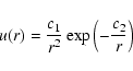
The initial radial ion velocity profile used is
 |
(10) |
where c1 = 0 in the stationary scenario,
![\begin{displaymath}Q =
c_3
\exp \left[ -\left( \frac{r-r_{Q,{\rm max}}}{\Delta r_Q} \right)^2 \right]
\exp \left[ \frac{c_2}{r} \right]
\end{displaymath}](/articles/aa/full_html/2009/12/aa10509-08/img79.gif) |
(11) |
where
| |
Figure 2: Ionospheric ion production rate profile used in all scenarios, and three initial radial velocity profiles used for inserting ionospheric ions in the different scenarios. Thick solid line: production rate of ionospheric ions. Dashed line: velocity profile for the stationary atmosphere scenario. Dashed-dotted line: velocity profile for the expanding atmosphere scenario. Dotted line: velocity profile for the high speed atmosphere scenario. The left-hand y axis is the ion production rate for all simulation runs. The right-hand y axis is the initial (radial) ionospheric outflow velocity. |
| Open with DEXTER | |
Thermospheric temperatures in close-in extrasolar giant planets such as HD 209458 b are expected to be ![]()
![]() (Seager et al. 2005; Yelle 2004). Although we are not modelling a giant planet here we use this as motivation for giving our ionospheric plasma an initial ion temperature of
(Seager et al. 2005; Yelle 2004). Although we are not modelling a giant planet here we use this as motivation for giving our ionospheric plasma an initial ion temperature of
![]() ,
equivalent to a thermal velocity of
,
equivalent to a thermal velocity of
![]() ,
and an electron temperature
,
and an electron temperature
![]() .
The initial electron temperature can not be set to a single well defined value since the electron fluid is adiabatic and is inserted under different pressures simultaneously.
.
The initial electron temperature can not be set to a single well defined value since the electron fluid is adiabatic and is inserted under different pressures simultaneously.
![\begin{figure}
\par\includegraphics[width=12cm,clip]{0509f3.eps}
\end{figure}](/articles/aa/full_html/2009/12/aa10509-08/img94.gif) |
Figure 3: Simulation results for the ionospheric plasma density in the stationary atmosphere scenario ( left), expanding atmosphere scenario ( middle) and high speed scenario ( right). The density is normalized to the background stellar wind density. Parts of the simulation box with zero ionospheric density have been removed for easier viewing. |
| Open with DEXTER | |
Finally, it remains to consider the neutral drag term in Eq. (1). We estimate (order of magnitude) and compare the electromagnetic force and the drag force for photoions in the rest frame of the stellar wind where E=0. Thus the electromagnetic acceleration is
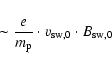 |
(12) |
and the drag acceleration is
| (13) |
respectively. The first estimation consists of known variables and is equal to
3 Results
![\begin{figure}
\par\includegraphics[width=16cm,clip]{0509f4co.ps}
\end{figure}](/articles/aa/full_html/2009/12/aa10509-08/img101.gif) |
Figure 4: Comparison of simulation results for the stationary atmosphere scenario ( left column), expanding atmosphere scenario ( middle column) and the high speed atmosphere scenario ( right column). The rows show magnetic field (row 1), stellar wind ion density (row 2), ionospheric ion density (row 3) and ionospheric ion velocity (row 4). All subfigures display the same equatorial plane through the center of the planet. All values are normalized to the background stellar wind. The white color in the third row represents zero density. |
| Open with DEXTER | |
![\begin{figure}
\par\includegraphics[width=16cm,clip]{0509f5co.ps}
\end{figure}](/articles/aa/full_html/2009/12/aa10509-08/img102.gif) |
Figure 5: Comparison of simulation results for the stationary atmosphere scenario ( left column), expanding atmosphere scenario ( middle column) and the high speed scenario ( right column). The rows show magnetic field (row 1), stellar wind ion density (row 2), ionospheric ion density (row 3) and ionospheric ion velocity (row 4). All subfigures display the same polar plane through the center of the planet. All values are normalized to the background stellar wind. The white color in the third row represents zero density. |
| Open with DEXTER | |
![\begin{figure}
\par\includegraphics[width=12cm,clip]{0509f6.eps}
\par\end{figure}](/articles/aa/full_html/2009/12/aa10509-08/img106.gif) |
Figure 6:
Comparison of simulation results along the x axis, parallel to the undisturbed stellar wind, and through the planet, between the stationary ( top), expanding ( middle) and high speed ( bottom) atmosphere runs. Thick solid line: stellar wind density. Dashed line: ionospheric density. Dotted line: ionospheric velocity in the x direction. Dash-dotted line: magnetic field in y direction. Thin solid line: ideal expansion density (nightside only). All values are normalized to the background stellar wind values. Plasma densities and ionospheric velocity have been removed in the interior of planet,
|
| Open with DEXTER | |
The results of our three simulation runs are illustrated in Figs. 3-6. Figure 3 is an overview of the results in the form of one 3D graph per scenario, each showing the ionospheric densities on three different cross sections. Figures 4 and 5 show the magnetic fields, plasma densities and ionospheric ion velocities in the equatorial and polar plane respectively. Lastly, Fig. 6 shows graphs of parameters along the x axis through the simulation box and the planet.
Starting by looking at Fig. 4, the equatorial plane, and Fig. 5, the polar plane, we can see that as expected in all scenarios, the planet is preceeded by a bow shock, clearly visible as a strong gradient in both magnetic field and stellar wind density. One can however see that the bow shock in the magnetic field is not as wide in the equatorial plane as in the polar plane. In particular it is cut off in the negative y direction in the equatorial plane, as can be expected since this part of the bow shock is nearly a parallel shock. Closer scrutiny reveals that also the bow shocks seen in stellar wind density in Figs. 4d-f are actually mirror asymmetric, since the negative y flanks are somewhat further downstream.
Looking again at Figs. 4 and 5, the bow shock in turn constitutes the upstream boundary of the magnetosheath, most clearly visible as a region of high stellar wind density. In Fig. 6 one can also see at the bow shock and magnetosheath how the stellar wind density and magnetic field match each other as theoretically expected until encountering the dayside ionosphere. In the equatorial plane, Figs. 4a-c, we see a very clear case of magnetic pile-up and draping. The magnetic pile-up region however has progressed not only into the dayside ionosphere in all three runs but also even into the planet for the stationary atmosphere run in Fig. 4a, likely because of the artificial magnetic diffusion which results from our smoothing procedure.
In the stationary atmosphere run, Fig. 4a, the magnetic draping in turn leads to the formation of two lobes in the equatorial plane, downstream of the planet, and what could be considered a thick current sheet in between. This is a very different picture compared to the configuration in the polar plane, Fig. 5a, where the same tail region is much wider and defined by its very weak magnetic field. In Figs. 4a-c and 5a-c however, we see that as expansion of the ionosphere is turned on, the current sheet greatly widens to a tail region similar in size to that in the polar plane.
Looking at the stellar wind density in Figs. 5d-f and to a lesser extent in the magnetic field in Figs. 5b and 5c, we also note the existence of artifacts in the form of reflections from the rear corners of the polar plane. The impact of these on the tail structure however is neglible.
The downstream boundary of the magnetosheath, the so called ion composition boundary (ICB, see e.g. Simon et al. 2007; Boesswetter et al. 2004), separates the incoming stellar wind from the ionospheric plasma. Looking at the stellar wind density on the dayside ICB in Figs. 4d-f and 5d-f, one can note that the ICB is less discrete for the stationary and expanding atmosphere run respectively but very discrete for the high speed atmosphere run. The picture is clearer when looking at the plasma densities along the x axis in Fig. 6. Apparently, in the stationary and expanding atmosphere runs, the stellar wind manages to penetrate fairly deeply into the ![]()
![]() thick plasma producing region surrounding the planet before being carried away around the planet, leading to ionospheric plasma being produced inside the stellar wind and thus a mixing of the two plasmas. In the high speed atmosphere run however, the ionospheric ram pressure is high enough to push the incoming stellar wind mostly out of this region, and thus not mix in the first place. Logically, as the same mixed or unmixed plasmas follow the ICB downstream, this pattern of ``fuzzy'' and discrete ICB should hold also for the ICB along the flanks. Looking at Figs. 4d-f and 5d-f, this seems to hold especially for the former. It is harder to say for Fig. 5f, since the different velocities on the different sides of the ICB here lead to the onset of a Kelvin-Helmholtz instability although not completely obvious if only analyzing the time step illustrated in this article. The ``lumpy'' structures on the ICB in Figs. 5h, 5i and 4i are also due to instability, most likely Kelvin-Helmholtz.
thick plasma producing region surrounding the planet before being carried away around the planet, leading to ionospheric plasma being produced inside the stellar wind and thus a mixing of the two plasmas. In the high speed atmosphere run however, the ionospheric ram pressure is high enough to push the incoming stellar wind mostly out of this region, and thus not mix in the first place. Logically, as the same mixed or unmixed plasmas follow the ICB downstream, this pattern of ``fuzzy'' and discrete ICB should hold also for the ICB along the flanks. Looking at Figs. 4d-f and 5d-f, this seems to hold especially for the former. It is harder to say for Fig. 5f, since the different velocities on the different sides of the ICB here lead to the onset of a Kelvin-Helmholtz instability although not completely obvious if only analyzing the time step illustrated in this article. The ``lumpy'' structures on the ICB in Figs. 5h, 5i and 4i are also due to instability, most likely Kelvin-Helmholtz.
Looking again at Fig. 6 and the effects of an expanding atmosphere, we see that it is clear that the added ionospheric ram pressure manages to displace all the major dayside structures upstream: bow shock, magnetic pile-up and ICB. Comparing the stationary atmosphere with the high speed atmosphere we see that the added ram pressure from the expanding ionosphere pushes the bow shock upstream by
![]() .
However, the initial dayside bulk velocity of the ionospheric plasma,
.
However, the initial dayside bulk velocity of the ionospheric plasma,
![]() for the expanding atmosphere and
for the expanding atmosphere and
![]() for the high-speed atmosphere, that is inherited from the postulated background atmosphere at ionization, is never really visible as a negative
for the high-speed atmosphere, that is inherited from the postulated background atmosphere at ionization, is never really visible as a negative
![]() in Fig. 6 as one might expect. The typical distance a hydrogen ion can travel before being diverted by the magnetic field is the gyration radius
in Fig. 6 as one might expect. The typical distance a hydrogen ion can travel before being diverted by the magnetic field is the gyration radius
 |
(14) |
where
Finally, we look at the ionospheric tail region, going from the stationary, to the expanding, to the high speed atmosphere run in Fig. 6. We there see that as opposed to on the dayside, the ionospheric tail velocity increases, which is quite natural since this is the only region where the ionosphere can continue to expand several ![]() away from the planet relatively undisturbed by the stellar wind. This also fits with the tail density decrease as plasma is more rapidly being transported out of the simulation box. In Fig. 6 we have for comparison also plotted the calculated density in the case of ideal spherically symmetric ionospheric expansion with the different (constant) expansion velocities for the respective scenarios. For the stationary atmosphere scenario we have used the thermal velocity of the ions. The agreement between the ideal expansion density with the simulation results is particularly good for high speed atmosphere scenario.
away from the planet relatively undisturbed by the stellar wind. This also fits with the tail density decrease as plasma is more rapidly being transported out of the simulation box. In Fig. 6 we have for comparison also plotted the calculated density in the case of ideal spherically symmetric ionospheric expansion with the different (constant) expansion velocities for the respective scenarios. For the stationary atmosphere scenario we have used the thermal velocity of the ions. The agreement between the ideal expansion density with the simulation results is particularly good for high speed atmosphere scenario.
Looking at Figs. 4g-l and 5g-l we can also see the structure of the tail change from being largely homogeneous in the stationary atmosphere run to dividing itself into two parts in the high speed atmosphere run: one undisturbed zone where the ionosphere can continue to expand and even maintain spherical symmetry, and a layer between this zone and the ICB which seems to be some kind of extension of the dayside ionosphere. Note the differences between the two planes: in the equatorial plane, the spherically symmetric tail region is wider, in the polar plane the ionospheric velocity in the layer is higher and thickens with distance from the planet.
Due to its weak magnetic field and thus large gyration radii of
![]() ,
the forementioned undisturbed tail region is that region where one could suspect kinetic effects to be significant on scales larger than one cell. The apparent spherical symmetry however suggests that no such exists.
,
the forementioned undisturbed tail region is that region where one could suspect kinetic effects to be significant on scales larger than one cell. The apparent spherical symmetry however suggests that no such exists.
Looking at the polar plane for the lower outflow velocities in Figs. 5j-l, i.e. stationary and expanding atmosphere runs, we note the existence of a thin layer of ionospheric ions with higher velocities on the ICB, accelerated by the interaction with the stellar wind plasma.
A further minor simulation result can be obtained by counting the number of ionospheric macroparticles which manage to leave the simulation box rather than be removed from the simulation by reaching the surface of the planet. This number, as a percentage of the total production rate of
![]() gives a hint to how large a fraction of the ionosphere that is lost to space rather than be ``recombined'' and returned to the lower parts of the planet's neutral atmosphere. We record 90% for the stationary atmosphere, and (virtually) 100% for the two other scenarios. Unsurprisingly, expansion prevents ions from reaching the planetary surface again.
gives a hint to how large a fraction of the ionosphere that is lost to space rather than be ``recombined'' and returned to the lower parts of the planet's neutral atmosphere. We record 90% for the stationary atmosphere, and (virtually) 100% for the two other scenarios. Unsurprisingly, expansion prevents ions from reaching the planetary surface again.
4 Discussion and conclusions
We have studied the influence of very rapidly expanding ionospheres on the stellar wind interaction for an unmagnetized close-in extrasolar terrestrial planet by comparing the simulation results for three different scenarios corresponding to a stationary atmosphere, an expanding atmosphere and an extremely expanding atmosphere (here referred to as ``high speed'' atmosphere). For this we have used a hybrid code, representing the plasma ions as macroparticles while treating the electrons as a charge-neutralizing, adiabatic fluid.
We have found that the added ionospheric ram pressure from the expanding ionosphere manages to displace all the major dayside structures upstream: bow shock, magnetic pile-up and ICB, as well as expand the entire interaction region. However, on the dayside the initial ionospheric expansion velocity never manifests itself as upstream bulk flow of plasma. Instead, the bulk velocity the ions are given upon insertion into the simulation box (i.e. at ionization) is very quickly thermalized in the already existing ionospheric plasma. The ram pressure exerted on the ionosphere from this process however still helps push the ionosphere upstream.
The high speed expansion qualitatively changes the tail region by creating a large nightside tail region unaffected by the stellar wind and largely void of electromagnetic fields where the ionosphere can continue to expand virtually undisturbed. Although in principle susceptible to large-scale kinetic effects (gyrations), this undisturbed tail region does not seem to display any such effects.
The postulated ``deep'' ionosphere (compared to solar system conditions) leads in the absence of expansion to more mixing of the ionospheric and stellar wind plasmas and to a partly less well defined ICB. We also note the onset of some Kelvin-Helmholtz instability for the two expanding atmosphere scenarios preventing a truly quasistationary state in our simulations.
Due to a lack of information on the nature of these ionospheres we have used a postulated ionosphere with inspiration from the expanding atmospheres of close-in extrasolar giant planets. We realize however that a more serious effort would require more intimate knowledge of these complex atmospheres. Future options for refining these kinds of simulations include constraining the ionosphere with some sort of rudimentary model, trying smaller angles between the stellar wind velocity and the stellar wind magnetic field as well as intrinsic planetary magnetic fields.
Acknowledgements
The authors acknowledge the fellowship of E.P.G.J. from the International Max Planck Research School (IMPRS) on Physical Processes in the Solar System and Beyond of the Max Planck Institute for Solar System Research (MPS) and the Universities of Braunschweig and Göttingen. The work of U.M. is supported by the Deutsche Forschungsgemeinschaft through grants MO539/13 and MO539/16.
References
- Bagdonat, T., & Motschmann, U. 2002, J. Comp. Phys., 183, 470 [NASA ADS] [CrossRef] (In the text)
- Baraffe, I., Selsis, F., Chabrier, G., et al. 2004, A&A, 419, L13 [NASA ADS] [CrossRef] [EDP Sciences]
- Baumjohann, W., & Treumann, R. A. 1996, Basic space plasma physics (London: Imperial College Press) (In the text)
- Boesswetter, A., Bagdonat, T., Motschmann, U., & Sauer, K. 2004, Annales Geophysicae, 22, 4363 [NASA ADS]
- Boesswetter, A., Simon, S., Bagdonat, T., et al. 2007, Annales Geophysicae, 25, 1851 [NASA ADS]
- Bordé, P., Rouan, D., & Léger, A. 2003, A&A, 405, 1137 [NASA ADS] [CrossRef] [EDP Sciences]
- Griessmeier, J.-M., Stadelmann, A., Penz, T., et al. 2004, A&A, 425, 753 [NASA ADS] [CrossRef] [EDP Sciences] (In the text)
- Holmström, M., Ekenbäck, A., Selsis, F., et al. 2008, Nature, 451, 970 [CrossRef]
- Hubbard, W. B., Hattori, M. F., Burrows, A., Hubeny, I., & Sudarsky, D. 2007, Icarus, 187, 358 [NASA ADS] [CrossRef]
- Ip, W.-H., Kopp, A., & Hu, J.-H. 2004, ApJ, 602, L53 [NASA ADS] [CrossRef]
- Kasting, J. F., & Pollack, J. B. 1983, Icarus, 53, 479 [NASA ADS] [CrossRef]
- Lammer, H., Selsis, F., Ribas, I., et al. 2003, ApJ, 598, L121 [NASA ADS] [CrossRef]
- Lammer, H., Selsis, F., Ribas, I., et al. 2004, in Stellar Structure and Habitable Planet Finding, ed. F. Favata, S. Aigrain, & A. Wilson, ESA SP, 538, 339
- Lecavelier des Etangs, A., Vidal-Madjar, A., McConnell, J. C., & Hébrard, G. 2004, A&A, 418, L1 [NASA ADS] [CrossRef] [EDP Sciences]
- Lin, D. N. C. 2006, Overview and prospective in theory and observation of planet formation (Planet Formation), 256
- Lipatov, A. S., Motschmann, U., Bagdonat, T., & Griessmeier, J.-M. 2005, Planet. Space Sci., 53, 423 [NASA ADS] [CrossRef] (In the text)
- Lovis, C., Mayor, M., & Udry, S. 2006, From hot Jupiters to hot Neptunes... and below (Planet Formation), 203
- Mann, G., Jansen, F., MacDowall, R. J., Kaiser, M. L., & Stone, R. G. 1999, A&A, 348, 614 [NASA ADS] (In the text)
- Marcy, G., Fischer, D. A., Butler, R. P., & Vogt, S. S. 2006, Properties of exoplanets: a Doppler study of 1330 stars (Planet Formation), 179
- Matthews, A. P. 1994, J. Comput. Phys., 112, 102 [NASA ADS] [CrossRef] (In the text)
- Parker, E. N. 1958, ApJ, 128, 664 [NASA ADS] [CrossRef] (In the text)
- Preusse, S., Kopp, A., Büchner, J., & Motschmann, U. 2005, A&A, 434, 1191 [NASA ADS] [CrossRef] [EDP Sciences]
- Preusse, S., Kopp, A., Büchner, J., & Motschmann, U. 2007, Planet. Space Sci., 55, 589 [NASA ADS] [CrossRef] (In the text)
- Raymond, S. N., Mandell, A. M., & Sigurdsson, S. 2006, Science, 313, 1413 [NASA ADS] [CrossRef]
- Schunk, R. W. & Nagy, A. F. 2000, Ionospheres: Physics, Plasma Physics, and Chemistry (Cambridge University Press) (In the text)
- Schwenn, R. 1990, Large-Scale Structure of the Interplanetary Medium (Physics of the Inner Heliosphere I), 99 (In the text)
- Schwenn, R., & Marsch, E. 1991, Physics of the Inner Heliosphere II. Particles, Waves and Turbulence (Berlin, Heidelberg, New York: Springer-Verlag) (In the text)
- Seager, S., Liang, M.-C., Parkinson, C. D., & Yung, Y. L. 2005, in Astrochemistry: Recent Successes and Current Challenges, ed. D. C. Lis, G. A. Blake, & E. Herbst, IAU Symp., 231, 491
- Simon, S., Boesswetter, A., Bagdonat, T., Motschmann, U., & Glassmeier, K.-H. 2006, Annales Geophysicae, 24, 1113 [NASA ADS]
- Simon, S., Boesswetter, A., Bagdonat, T., & Motschmann, U. 2007, Annales Geophysicae, 25, 99 [NASA ADS]
- Sonett, C. P., Coleman, P. J., & Wilcox, J. M., 1972, Solar Wind, National Aeronautics and Space Administration, NASA SP-308 (In the text)
- Tian, F., Toon, O. B., Pavlov, A. A., & De Sterck, H. 2005, ApJ, 621, 1049 [NASA ADS] [CrossRef]
- Vidal-Madjar, A., Lecavelier des Etangs, A., Désert, J.-M., et al. 2003, Nature, 422, 143 [NASA ADS] [CrossRef]
- Vidal-Madjar, A., Désert, J.-M., Lecavelier des Etangs, A., et al. 2004, ApJ, 604, L69 [NASA ADS] [CrossRef]
- Yelle, R. V. 2004, Icarus, 170, 167 [NASA ADS] [CrossRef]
- Zarka, P., Treumann, R. A., Ryabov, B. P., & Ryabov, V. B. 2001, Ap&SS, 277, 293 [NASA ADS] [CrossRef] (In the text)
Footnotes
- ... planets
![[*]](/icons/foot_motif.gif)
- Retrieved on July 2nd 2008 from The Extrasolar Planets Encyclopaedia on http://exoplanet.eu/.
All Figures
| |
Figure 1:
Cartoon showing the coordinate axes of the simulation box.
|
| Open with DEXTER | |
| In the text | |
| |
Figure 2: Ionospheric ion production rate profile used in all scenarios, and three initial radial velocity profiles used for inserting ionospheric ions in the different scenarios. Thick solid line: production rate of ionospheric ions. Dashed line: velocity profile for the stationary atmosphere scenario. Dashed-dotted line: velocity profile for the expanding atmosphere scenario. Dotted line: velocity profile for the high speed atmosphere scenario. The left-hand y axis is the ion production rate for all simulation runs. The right-hand y axis is the initial (radial) ionospheric outflow velocity. |
| Open with DEXTER | |
| In the text | |
| |
Figure 3: Simulation results for the ionospheric plasma density in the stationary atmosphere scenario ( left), expanding atmosphere scenario ( middle) and high speed scenario ( right). The density is normalized to the background stellar wind density. Parts of the simulation box with zero ionospheric density have been removed for easier viewing. |
| Open with DEXTER | |
| In the text | |
| |
Figure 4: Comparison of simulation results for the stationary atmosphere scenario ( left column), expanding atmosphere scenario ( middle column) and the high speed atmosphere scenario ( right column). The rows show magnetic field (row 1), stellar wind ion density (row 2), ionospheric ion density (row 3) and ionospheric ion velocity (row 4). All subfigures display the same equatorial plane through the center of the planet. All values are normalized to the background stellar wind. The white color in the third row represents zero density. |
| Open with DEXTER | |
| In the text | |
| |
Figure 5: Comparison of simulation results for the stationary atmosphere scenario ( left column), expanding atmosphere scenario ( middle column) and the high speed scenario ( right column). The rows show magnetic field (row 1), stellar wind ion density (row 2), ionospheric ion density (row 3) and ionospheric ion velocity (row 4). All subfigures display the same polar plane through the center of the planet. All values are normalized to the background stellar wind. The white color in the third row represents zero density. |
| Open with DEXTER | |
| In the text | |
| |
Figure 6:
Comparison of simulation results along the x axis, parallel to the undisturbed stellar wind, and through the planet, between the stationary ( top), expanding ( middle) and high speed ( bottom) atmosphere runs. Thick solid line: stellar wind density. Dashed line: ionospheric density. Dotted line: ionospheric velocity in the x direction. Dash-dotted line: magnetic field in y direction. Thin solid line: ideal expansion density (nightside only). All values are normalized to the background stellar wind values. Plasma densities and ionospheric velocity have been removed in the interior of planet,
|
| Open with DEXTER | |
| In the text | |
Copyright ESO 2009
Current usage metrics show cumulative count of Article Views (full-text article views including HTML views, PDF and ePub downloads, according to the available data) and Abstracts Views on Vision4Press platform.
Data correspond to usage on the plateform after 2015. The current usage metrics is available 48-96 hours after online publication and is updated daily on week days.
Initial download of the metrics may take a while.