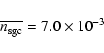
| Issue |
A&A
Volume 496, Number 1, March II 2009
|
|
|---|---|---|
| Page(s) | 7 - 23 | |
| Section | Cosmology (including clusters of galaxies) | |
| DOI | https://doi.org/10.1051/0004-6361:200810575 | |
| Published online | 14 January 2009 | |
Large-scale fluctuations in the distribution of galaxies from the two-degree galaxy redshift survey
F. Sylos Labini1,2 - N. L. Vasilyev3 - Y. V. Baryshev3
1 - Centro Studi e Ricerche Enrico Fermi, via Panisperna 89 A, Compendio del Viminale, 00184 Rome, Italy
2 - Istituto dei Sistemi Complessi CNR, via dei Taurini 19, 00185 Rome, Italy
3 - Institute of Astronomy, St.Petersburg State University, Staryj Peterhoff, 198504,
St. Petersburg, Russia
Received 11 July 2008 / Accepted 5 December 2008
Abstract
We study statistical properties of galaxy structures in
several samples extracted from the two-degree galaxy redshift survey (2dFRGS). In
particular, we measure conditional fluctuations by means of the
scale-length method and determined their probability
distribution. In this way we find that galaxy distribution in these
samples is characterized by large amplitude fluctuations with a
large spatial extension, whose size is only limited by the sample's
boundaries. These fluctuations are quite typical and persistent in
the sample's volumes, and they are detected in two independent
regions in the northern and southern galactic caps. We discuss the
relation of the scale-length method to several statistical
quantities, such as counts of galaxies as a function of redshift and
apparent magnitude. We confirm previous results, which have
determined by magnitude and redshift counts that there are
fluctuations of about 30% between the southern and the northern
galactic caps and we relate explicitly these counts to structures in
redshift space. We show that the estimation of fluctuation amplitude
normalized to the sample density is biased by systematic effects,
which we discuss in detail. We consider the type of fluctuations
predicted by standard cosmological models of structure formation in
the linear regime and, to study nonlinear clustering, we analyze
several samples of mock-galaxy catalogs generated from the distribution of dark matter in cosmological N-body simulations. In this way we conclude that the galaxy fluctuations present in these samples are too large in amplitude and too extended in space to be compatible with the predictions of the standard models of structure formation.
Key words: cosmology: observations - cosmology: large-scale structure of Universe
1 Introduction
In one of his seminal papers de Vaucouleurs (1970) put into a historical
perspective the problem of galaxy large-scale structures and the
question about the scale where galaxy distribution turns to
homogeneity![]() . He points out
that observations have first found that galaxies are not randomly
distributed, then that in the fifties the same property was assigned
to cluster centers, and finally that at the end of the sixties the
discovery of super-clusters has still enlarged the scale of structures
in the universe, thus pushing the scale where the approach to
homogeneity occurs to larger and larger scales.
. He points out
that observations have first found that galaxies are not randomly
distributed, then that in the fifties the same property was assigned
to cluster centers, and finally that at the end of the sixties the
discovery of super-clusters has still enlarged the scale of structures
in the universe, thus pushing the scale where the approach to
homogeneity occurs to larger and larger scales.
In the past twenty years many observations have been dedicated to the
study of the large-scale distributions of galaxies
(Falco et al. 1999; Huchra et al. 1983; Giovanelli & Haynes 1993; da Costa et al. 1988; Colless et al. 2001; Shectman et al. 1996; York et al. 2000). Despite the fact that
large-scale galaxy structures, of about several hundred Mpc/h
size![]() , have been observed
(Geller & Huchra 1989; Giovanelli & Haynes 1993; Gott et al. 2005; de Lapparent Huchra & Geller 1986) to be the typical feature of the
distribution of visible matter in the local universe, the statistical
analysis measuring their properties has identified a characteristic
scale that has only slightly changed since its discovery forty years
ago in angular catalogs. This scale, r0, was measured to be the one
at which fluctuations in the galaxy density field are about twice the
value of the sample density and it was indeed determined to be
, have been observed
(Geller & Huchra 1989; Giovanelli & Haynes 1993; Gott et al. 2005; de Lapparent Huchra & Geller 1986) to be the typical feature of the
distribution of visible matter in the local universe, the statistical
analysis measuring their properties has identified a characteristic
scale that has only slightly changed since its discovery forty years
ago in angular catalogs. This scale, r0, was measured to be the one
at which fluctuations in the galaxy density field are about twice the
value of the sample density and it was indeed determined to be
![]() Mpc/h in the Shane and Wirtanen angular catalog
(Totsuji & Kihara 1969). Subsequent measurements of this scale - see
e.g. Davis & Peebles (1983), Davis et al. (1988), Park et al. (1994), Benoist et al. (1996), Norberg et al. (2001, 2002b), Zehavi et al. (2004) - found a similar value,
although in several samples larger values of r0 have been found
(i.e.,
Mpc/h in the Shane and Wirtanen angular catalog
(Totsuji & Kihara 1969). Subsequent measurements of this scale - see
e.g. Davis & Peebles (1983), Davis et al. (1988), Park et al. (1994), Benoist et al. (1996), Norberg et al. (2001, 2002b), Zehavi et al. (2004) - found a similar value,
although in several samples larger values of r0 have been found
(i.e.,
![]() -12 Mpc/h). This variation was then ascribed to
a luminosity dependent effect - see e.g.
Davis et al. (1988), Park et al. (1994), Benoist et al. (1996), Zehavi et al. (2002).
-12 Mpc/h). This variation was then ascribed to
a luminosity dependent effect - see e.g.
Davis et al. (1988), Park et al. (1994), Benoist et al. (1996), Zehavi et al. (2002).
Theoretical models of galaxy formation, like the cold dark matter
(CDM) one (see Peacock 1999) are able to predict the scale r0 once it is given the amplitude and correlation properties of
fluctuations of the initial conditions in the early universe. The
normalization of the matter initial condition can be obtained by
measuring the amplitude and correlation properties of the
anisotropies of the cosmic microwave background radiation
(CMBR). Then by calculating the evolution of small density
fluctuations in the linear perturbation analysis of a
self-gravitating fluid in an expanding universe, it is possible to
predict the scale r0 today. This turns out, in current models such
as the CDM ones, to be
![]() Mpc/h (Springel et al. 2005). On
scales r<r0 models are unable to make precise predictions of the
shape of the correlation function because gravitational clustering in
the nonlinear regime is difficult to be treated. Gravitational N-body
simulations are then used to investigate structure formation in the
nonlinear phase. In addition, given that models predict, for
r>r0, a precise type of small amplitude fluctuations, it is
possible to simply relate, by using the linear perturbation analysis
mentioned above, the properties of fluctuations in the present matter
density field to those in the initial conditions. In a certain range
of scales greater than r0, small amplitude. fluctuations should
have still positive correlations. Particularly, for
Mpc/h (Springel et al. 2005). On
scales r<r0 models are unable to make precise predictions of the
shape of the correlation function because gravitational clustering in
the nonlinear regime is difficult to be treated. Gravitational N-body
simulations are then used to investigate structure formation in the
nonlinear phase. In addition, given that models predict, for
r>r0, a precise type of small amplitude fluctuations, it is
possible to simply relate, by using the linear perturbation analysis
mentioned above, the properties of fluctuations in the present matter
density field to those in the initial conditions. In a certain range
of scales greater than r0, small amplitude. fluctuations should
have still positive correlations. Particularly, for
![]() ,
fluctuations have very small amplitude and weak positive correlations
(see Sylos Labini & Vasilyev 2008). On even larger scales
,
fluctuations have very small amplitude and weak positive correlations
(see Sylos Labini & Vasilyev 2008). On even larger scales
![]() (where this is
estimated from CMBR measurements to be
(where this is
estimated from CMBR measurements to be
![]() Mpc/h), all
models predict that the matter density field presents anti-correlations that tend to zero with a (negative) power-law
behavior of the type -r-4 (Sylos Labini & Vasilyev 2008; Gabrielli et al. 2002). This negative
power-law tail corresponds in real-space to the linear dependence of
the matter power-spectrum (PS) on the wave-number; i.e.,
Mpc/h), all
models predict that the matter density field presents anti-correlations that tend to zero with a (negative) power-law
behavior of the type -r-4 (Sylos Labini & Vasilyev 2008; Gabrielli et al. 2002). This negative
power-law tail corresponds in real-space to the linear dependence of
the matter power-spectrum (PS) on the wave-number; i.e.,
![]() .
The former represents a behavior that can be interpreted as a
consistency requirement for the properties of density fluctuations in
Friedmann-Robertson-Walker models (Gabrielli et al. 2002). Because of the
change in sign of the correlation function at
.
The former represents a behavior that can be interpreted as a
consistency requirement for the properties of density fluctuations in
Friedmann-Robertson-Walker models (Gabrielli et al. 2002). Because of the
change in sign of the correlation function at ![]() ,
this
length-scale represents the cut-off in the size of weak amplitude
structures in standard models. Thus, in the regime where fluctuations
are small and have weak positive correlations; i.e., for
,
this
length-scale represents the cut-off in the size of weak amplitude
structures in standard models. Thus, in the regime where fluctuations
are small and have weak positive correlations; i.e., for
![]() ,
the present matter-density field reflects the imprint of the
initial conditions.
,
the present matter-density field reflects the imprint of the
initial conditions.
The fundamental test for current models of galaxy formation then
concerns whether density fluctuations on large scales (i.e., r>10 Mpc/h) have small amplitude or not. Another important question
concerns the detection of anti-correlations on scales of
![]() Mpc/h (Sylos Labini & Vasilyev 2008). The primary problem to be
considered in this respect concerns the statistical methods used to
measure the amplitude of fluctuations and the range of
correlations. There has been intense debate in the past decade
concerning this crucial point
(Wu et al. 1999; Baryshev & Teerikorpi 2005; Sylos Labini et al. 2008; Gabrielli et al. 2005; Sylos Labini et al. 1998; Hogg et al. 2005).
Before one determines the amplitude of fluctuations in a given volume
with respect to the sample density, one must have firstly tested that
the former quantity is stable; i.e., that it does not depend on the
sample size and/or it does not present large fluctuations in
different samples containing the same type of objects. Indeed, in
case the distribution presents structures and fluctuations on all
scales in a given sample (i.e., it is inhomogeneous) the sample
density is not a well-defined descriptor (Sylos Labini et al. 2008,1998). In
this situation all statistical quantities that are normalized to the
sample density are affected by systematic effects. For this reason,
prior to the characterization of fluctuations with respect to the
sample density, a fundamental test consists in measuring conditional
correlation properties (Gabrielli et al. 2005). It has been found that
conditional statistical quantities, such as the conditional number of
points in spheres, indeed show scaling properties on small
scales r <20 Mpc/h, e.g., the former grows as a function of
distance more slowly than the volume
(Sylos Labini et al. 2007,2008; Vasilyev et al. 2006; Sylos Labini et al. 1998; Hogg et al. 2005). This result implies
that unconditional quantities are affected by systematic finite-size
effects and thus do not give a reliable and meaningful estimation of
correlations and amplitude of fluctuations. In this situation the
length scale r0 can be an artifact of a statistical analysis,
which assumes that the sample average is a meaningful estimation of
the asymptotic density; i.e., it assumes that the distribution is
homogeneous and that fluctuations have a small amplitude well inside
the sample volume.
Mpc/h (Sylos Labini & Vasilyev 2008). The primary problem to be
considered in this respect concerns the statistical methods used to
measure the amplitude of fluctuations and the range of
correlations. There has been intense debate in the past decade
concerning this crucial point
(Wu et al. 1999; Baryshev & Teerikorpi 2005; Sylos Labini et al. 2008; Gabrielli et al. 2005; Sylos Labini et al. 1998; Hogg et al. 2005).
Before one determines the amplitude of fluctuations in a given volume
with respect to the sample density, one must have firstly tested that
the former quantity is stable; i.e., that it does not depend on the
sample size and/or it does not present large fluctuations in
different samples containing the same type of objects. Indeed, in
case the distribution presents structures and fluctuations on all
scales in a given sample (i.e., it is inhomogeneous) the sample
density is not a well-defined descriptor (Sylos Labini et al. 2008,1998). In
this situation all statistical quantities that are normalized to the
sample density are affected by systematic effects. For this reason,
prior to the characterization of fluctuations with respect to the
sample density, a fundamental test consists in measuring conditional
correlation properties (Gabrielli et al. 2005). It has been found that
conditional statistical quantities, such as the conditional number of
points in spheres, indeed show scaling properties on small
scales r <20 Mpc/h, e.g., the former grows as a function of
distance more slowly than the volume
(Sylos Labini et al. 2007,2008; Vasilyev et al. 2006; Sylos Labini et al. 1998; Hogg et al. 2005). This result implies
that unconditional quantities are affected by systematic finite-size
effects and thus do not give a reliable and meaningful estimation of
correlations and amplitude of fluctuations. In this situation the
length scale r0 can be an artifact of a statistical analysis,
which assumes that the sample average is a meaningful estimation of
the asymptotic density; i.e., it assumes that the distribution is
homogeneous and that fluctuations have a small amplitude well inside
the sample volume.
While estimations of real-space correlation properties can be affected
by finite-size effects, this is not the case when one counts galaxies
as a function of redshift or apparent magnitude. In this case indeed
one does not normalize statistical quantities to the sample average,
and large fluctuations have been found both in redshift
(Chiaki et al. 2003; Kerscher et al. 1999) and angular surveys
(see Picard 1991; Frith et al. 2003). In particular, in a CCD survey of
bright galaxies within the northern and southern strips of the 2dF
galaxy redshift survey (2dFGRS) conclusive evidence is found of
fluctuations of ![]() 30% in galaxy counts as a function
of apparent magnitude (Busswell et al. 2004).
Since in the angular region toward the southern galactic cap (SGC) a
deficiency, with respect to the northern galactic cap (NGC) in the
counts below magnitude
30% in galaxy counts as a function
of apparent magnitude (Busswell et al. 2004).
Since in the angular region toward the southern galactic cap (SGC) a
deficiency, with respect to the northern galactic cap (NGC) in the
counts below magnitude ![]() 17 (in the B filter) was found,
persisting over the full area of the APM and APMBGC catalogs, this
would be evidence that there is a large void with a radius of about
150 Mpc/h, implying that there is more excess large-scale power than
detected in the 2dFGRS correlation function
17 (in the B filter) was found,
persisting over the full area of the APM and APMBGC catalogs, this
would be evidence that there is a large void with a radius of about
150 Mpc/h, implying that there is more excess large-scale power than
detected in the 2dFGRS correlation function![]() (Norberg et al. 2002b,2001) or expected in the CDM models. It is
indeed evident that, because of the difference in the counts'
amplitude, and thus in the sample density, between the NGC and the SGC
samples, any estimation of the sample density is not stable. Thus the
problems for the normalization of fluctuations amplitude to the
estimation of the sample density should be studied in great detail.
(Norberg et al. 2002b,2001) or expected in the CDM models. It is
indeed evident that, because of the difference in the counts'
amplitude, and thus in the sample density, between the NGC and the SGC
samples, any estimation of the sample density is not stable. Thus the
problems for the normalization of fluctuations amplitude to the
estimation of the sample density should be studied in great detail.
In this paper we use the 2dFGRS to study fluctuations in galaxy distribution on large scales and to determine their statistical properties in redshift and magnitude space. Our aim is to employ statistical descriptors that do not, implicitly or explicitly, make use of the normalization of fluctuations to the sample average, thus avoiding the a-priori assumption of homogeneity inside a given sample. Thus we determine conditional statistical properties, thereby expanding our previous findings in this same survey (Vasilyev et al. 2006; Sylos Labini et al. 2009). We find that the puzzle of the coexistence of difference in densities in the NGC and SGC volumes on large spatial scales with a relatively small typical length scale of a few Mpc, can be understood as due to finite size effects in the estimation of the correlation function.
The paper is organized as follows. In Sect. 2 we discuss the 2dFGRS data and the procedure used to construct the sub samples for the statistical analysis. The methods for characterizing homogeneous and heterogeneous distributions are briefly reviewed in Sect. 3. In Sect. 4 we present the main results of the analysis and consider in detail the problems related to estimating fluctuations' amplitude normalized to the sample density. The properties of fluctuations of the matter density field predicted by theoretical models, in the linear regime, are briefly reviewed in Sect. 5. Then, to study expected nonlinear fluctuations in standard theoretical models, we analyze the properties of mock-galaxy catalogs, generated from the dark matter density fields stemming from a cosmological N-body simulation - the Millennium Run by Springel et al. (2005). Finally in Sect. 6 we discuss the results of the analysis of the 2dFGRS samples and outline our main conclusions.
2 The 2dFGRS samples
The 2dFGRS (Colless et al. 2001) measured redshifts for more than
220 000 galaxies in two strips in the SGC and in the NGC. The
median redshift is
![]() .
The apparent magnitude corrected for
galactic extinction in the bJ filter is limited to
14.0<bJ<19.45. The selection of the samples used in the analysis
is described in detail in Vasilyev et al. (2006). Here we briefly
summarize the main points.
.
The apparent magnitude corrected for
galactic extinction in the bJ filter is limited to
14.0<bJ<19.45. The selection of the samples used in the analysis
is described in detail in Vasilyev et al. (2006). Here we briefly
summarize the main points.
- To avoid the effect of the irregular edges of the survey, we
selected two rectangular regions: in the SGC there is a slice of
size
 limited by
 ,
,
 ,
while the
NGC slice is smaller, i.e.,
,
while the
NGC slice is smaller, i.e.,
 ,
with
limits
,
with
limits
 ,
,
 (coordinates are equatorial). The solid angles are
 steradians for the SGC and the NGC slices.
- We selected galaxies in the redshift interval
 ,
with redshift quality parameter larger or equal to three, in
order to get high quality redshifts (Hawkins et al. 2003).
,
with redshift quality parameter larger or equal to three, in
order to get high quality redshifts (Hawkins et al. 2003).
- We did not use a correction for the redshift-completeness mask
and for the fiber collision effects. In fact, completeness varies
mostly near the survey edges, which are excluded in our sample. We
assumed that fiber collisions do not make a noticeable change in the
small-scale correlation properties given that we set our lower
cut-off to 0.5 Mpc/h, which is larger than the 0.1 Mpc/h used by
Hawkins et al. (2003).
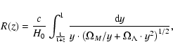
- The metric distance is usually computed as in Zehavi et al. (2002):
where we used the standard model parameters and
and
 ,
and c is the light speed.
,
and c is the light speed.
- The absolute magnitude was computed as in Zehavi et al. (2002):
where K(z) is the K-correction term (Hogg et al. 2002). - To calculate the K-correction K(z) we used relations obtained by Madgwick et al. (2002) and we applied them as in Vasilyev et al. (2006).
- The volume-limited (VL) samples were identified by two limits in the metric distance
 and two corresponding
limits in the absolute magnitude
and two corresponding
limits in the absolute magnitude  and
and  .
In
Table 1 we report the properties of the VL
samples.
.
In
Table 1 we report the properties of the VL
samples.
![\begin{displaymath}
M = b_J - 5 \cdot \log_{10}\left[R(z) \cdot (1+z)\right] - K(z) - 25,
\end{displaymath}](/articles/aa/full_html/2009/10/aa10575-08/img35.gif)
Table 1:
Main properties of the obtained VL samples. ![]() ,
,
![]() are the chosen limits for the metric distance;
are the chosen limits for the metric distance;
![]() are the corresponding limits in the absolute magnitude;
are the corresponding limits in the absolute magnitude; ![]() is the number of galaxies in the sample.
is the number of galaxies in the sample.
As a self-consistent test, we note below that the statistical analysis in the samples constructed with less conservative cuts agree with previous determinations for what concerns the galaxy counts as a function of apparent magnitude (Busswell et al. 2004; Norberg et al. 2002a), the redshift distribution (Ratcliffe et al. 1998; Busswell et al. 2004), and the standard two-point correlation function (Norberg et al. 2002b,2001).
Table 2: As Table 1 but for the case of more conservative cuts in apparent magnitudes; i.e. 14.5<bJ<19.3, were used for selecting the galaxies.
3 Statistical methods
In this section we review the main properties of stationary stochastic point processes. These include both the ones that have a strictly positive ensemble average density and those which have it equal to zero.This discussion clarifies what the useful statistical methods are in both cases for analyzing a finite sample. A more exhaustive treatment can be found in Gabrielli et al. (2005).
3.1 Volume average, ensemble average, and self-averaging property
The problem of the statistical characterization of correlations and fluctuations of a stochastic distribution of points in a finite sample of volume V can be rephrased as the problem of measuring volume-averaged statistical quantities. The basic issue concerns whether or not these are meaningful descriptors, i.e., whether or not they give stable statistical estimations of ensemble averaged quantities. In this respect one has to consider various problems that maybe clarified after the definition of the general probabilistic properties of stochastic point processes.
First of all, we need to define the ensemble properties. In general it
is assumed that galaxy distribution is a stationary stochastic
process, which means that it is statistically, translationally, and
rotationally invariant; i.e., it satisfies the condition of spatial
statistical isotropy and homogeneity in order to avoid special points
or directions![]() . Stationary stochastic distributions also satisfy these conditions when they have zero average density in the infinite
volume limit (Gabrielli et al. 2005).
. Stationary stochastic distributions also satisfy these conditions when they have zero average density in the infinite
volume limit (Gabrielli et al. 2005).
Due to the assumption of ergodicity (i.e., the ensemble average is
equal to the infinite volume average), the existence of a well-defined
average density implies that, for a single realization of the mass
distribution, the following limit is well-defined:
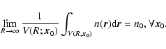
where
Keeping these mathematical properties in mind we have to consider the situation occurring when in a finite sample, of size ![]() V1/3, the distribution is not homogeneous. In this case the estimator of the average mass density gives a large relative error with respect to
the ensemble value making it systematically biased. This implies that only statistical averages conditioned to the fact that the origin of coordinates is a point of the set are well-defined.
V1/3, the distribution is not homogeneous. In this case the estimator of the average mass density gives a large relative error with respect to
the ensemble value making it systematically biased. This implies that only statistical averages conditioned to the fact that the origin of coordinates is a point of the set are well-defined.
Clearly a distribution can be inhomogeneous up to a length scale ![]()
![]() and homogeneous for
and homogeneous for
![]() .
Then for
.
Then for
![]() the distribution
is characterized by large fluctuations, and the average density is not a well-defined quantity if it is estimated in samples of size
the distribution
is characterized by large fluctuations, and the average density is not a well-defined quantity if it is estimated in samples of size
![]() .
Instead density fluctuations are small for
.
Instead density fluctuations are small for
![]() and the sample density converges to the asymptotic (or ensemble) value
when the sample volume is such that
and the sample density converges to the asymptotic (or ensemble) value
when the sample volume is such that
![]() .
The precise behavior of this convergence is determined by the (weak) two-point correlation properties of the distributions, and the
convergence will be slower when correlations are long-range (Gabrielli et al. 2005).
.
The precise behavior of this convergence is determined by the (weak) two-point correlation properties of the distributions, and the
convergence will be slower when correlations are long-range (Gabrielli et al. 2005).
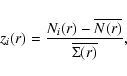
3.2 Probability distribution of conditional fluctuations
In Sylos Labini et al. (2008) we have introduced the scale-length (SL) analysis. This consists in determining the number N(r;Ri) of galaxies in spheres of radius r, centered on the ith galaxy![]() whose distance from the origin is Ri; that is,
whose distance from the origin is Ri; that is,
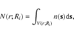
where the integral is performed over the spherical volume V(r;Ri) of radius r centered on the ith galaxy at distance Ri from the origin, and
When Eq. (4) is averaged over the whole sample, it gives an estimate of the average conditional number of galaxies in spheres of radius r
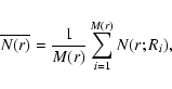
where the sum is extended to the M(r) galaxies, the ith at radial distance Ri from us, whose separation from the boundaries of the sample is less than or equal to r. In this way when r grows the number of values M(r) over which the mean in Eq. (5) is performed decreases with r, because only those galaxies for which the sphere is fully included in the sample volume are considered as centers.
This estimator, known as the full-shell estimator
(Kerscher 1999; Gabrielli et al. 2005; Sylos Labini et al. 1998), has the advantage of making the weakest
a-priori assumptions about the properties of the distribution outside
the sample volume. Indeed one may use incomplete spheres by counting
the number of galaxies inside a portion of a sphere and weighting this
for the corresponding volume of the spherical portion
(Kerscher 1999). However, this method implicitly uses the assumption
that what is inside the incomplete sphere is a statistically
meaningful estimate of the distribution in the whole spherical
volume. This is incorrect when the distribution presents large
fluctuations. For example in the part of a spherical volume that lies
outside the sample boundaries, there can be a void or a large-scale
structure and in this situation the weighted estimation is biased
(Gabrielli et al. 2005). When the full-shell estimator is used, one should
consider that there is an intrinsic selection effect related to the
geometry of the samples, which are small portions of spheres. When ris large only the more distant part of the sample is explored by the
volume average (Sylos Labini et al. 2008; Gabrielli et al. 2005). Indeed, for large-sphere radii,
M(r) decreases and the location of the galaxies contributing to the
average in Eq. (5) is mostly placed at radial distance in the
range ![]()
![]() ,
,
![]() from the radial boundaries of
the sample at
from the radial boundaries of
the sample at ![]() ,
,
![]() .
Given the geometry
of the samples for large r, galaxies contributing to M(r) will
also lie toward the center of the spherical portion.
.
Given the geometry
of the samples for large r, galaxies contributing to M(r) will
also lie toward the center of the spherical portion.
When Eq. (5) scales as

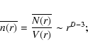
and D=3, the distribution is homogeneous, while for D<3 it has long-range power-law correlations (Gabrielli et al. 2005). The scaling of Eq. (6) with D<3 can be interpreted as the signature that the distribution is a fractal; however there are point distributions that, by construction, are not fractal objects but which may exhibit a scaling of the type given by Eq. (6) (see Gabrielli et al. 2005).
From Eq. (6) we obtain that, in general, for D<3 the conditional density scales as
in this situation the average density is not a well defined quantity and the sample density is depends on the sample size; i.e., it does not give a meaningful estimation of the ensemble average density.
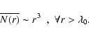
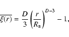
When a distribution is fractal (or generally inhomogeneous) on small scales and homogeneous on large scales, then we can identify the homogeneity scale ![]() to be the scale such that (Gabrielli et al. 2005)
to be the scale such that (Gabrielli et al. 2005)
Depending on the details of the crossover from the strongly correlated regime at
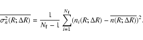
The estimator defined by Eq. (5) gives the first moment (i.e., the
average number of points in spheres of radius r) of the PDF of
conditional fluctuations f(N;r) computed, at fixed r, from the
values
![]() .
This is generally different from
the PDF of unconditional fluctuations - considered by, e.g.,
Saslaw (2000) - both for homogeneous and inhomogeneous
distributions, the difference being more important in the former case.
.
This is generally different from
the PDF of unconditional fluctuations - considered by, e.g.,
Saslaw (2000) - both for homogeneous and inhomogeneous
distributions, the difference being more important in the former case.
When a distribution becomes homogeneous; i.e., Eq. (7) is satisfied, the PDF is expected to converge in a finite volume to a Gaussian function![]() (Gabrielli et al. 2005); i.e.,
(Gabrielli et al. 2005); i.e.,
![\begin{displaymath}
f(N;r \gg \lambda_0) \simeq \frac{1} {\sqrt{2 \pi
\overline...
...r) -
\overline{N(r)}]^2} {2 \overline{ \Sigma^2(r)}} \right),
\end{displaymath}](/articles/aa/full_html/2009/10/aa10575-08/img64.gif)
where
The second moment of f(N,V) gives the conditional variance. For inhomogeneous distributions, this is such that
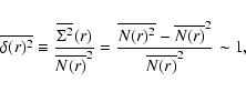
where the last equality means that fluctuations are persistent (Gabrielli & Sylos Labini 2001). On the other hand, for homogeneous distributions with any kind of small-amplitude correlations, we find that (Gabrielli & Sylos Labini 2001)
 |
(11) |
When the sample density
In this case the homogeneity scale can be, for instance, defined as the scale beyond which
4 Results from the 2dFGRS
In this section we present the results of the statistical analysis of
the VL samples of the 2dFGRS catalog discussed in
Sect. 2. We start by presenting the SL analysis to
then move to the description of the determination of the PDF of
conditional fluctuations. Furthermore, we consider its first moment;
i.e., the average number of points in spheres. To illustrate the
usefulness of the SL analysis, we consider its relation to the counts
of galaxies as a function of radial distance and of apparent
magnitude. This allows us to discuss in detail the relation between
small scale two-point correlations and large scale properties of
fluctuations in the galaxy density field. We then consider the
finite-size effects that systematically affect the determination of
fluctuations amplitude normalized to the sample density. In addition
we compute the average of the SL determinations
![]() in bins of radial distance. The comparison of the behaviors in the NGC and SGC slices allows us to place a lower limit on the homogeneity scale.
in bins of radial distance. The comparison of the behaviors in the NGC and SGC slices allows us to place a lower limit on the homogeneity scale.
4.1 The scale-length analysis
In Figs. 1-4 the behavior of the SL analysis is shown in the four 2dFGRS samples we considered. One may note that in all cases there are large density fluctuations in the correspondence of the location of galaxy large-scale structures. In Fig. 5 a three-dimensional plot is shown of the same SL analysis reported in Fig. 4. One may see how well structures are identified by this analysis.
The number of points M(r) over which N(r;Ri) is computed, as a function of the sphere radius r is shown in Fig. 6: when the sphere radius r gets larger, the M(r) decreases quite rapidly. This is due to the geometrical selection effect previously discussed. In addition, the solid angle of the SGC slice is twice that of the NGC slice, and thus for r>20 Mpc/h, there are more center points in the SGC samples than in the NGC ones.
Let us briefly discuss the main features that we detect in the various samples![]()
![\begin{figure}
\par\includegraphics*[angle=0, width=9cm]{0575Fig1-NEW.eps}
\end{figure}](/articles/aa/full_html/2009/10/aa10575-08/img73.gif) |
Figure 1: From top to bottom the SL analysis for the sample NGC400 with r=5,10 Mpc/h. |
| Open with DEXTER | |
![\begin{figure}
\par\includegraphics*[angle=0, width=9cm]{0575Fig2-NEW.eps}
\end{figure}](/articles/aa/full_html/2009/10/aa10575-08/img74.gif) |
Figure 2: The same as Fig. 1 but now for the sample NGC550 with r=10,15 Mpc/h. |
| Open with DEXTER | |
![\begin{figure}
\par\includegraphics*[angle=0, width=9cm]{0575Fig3-NEW.eps}
\end{figure}](/articles/aa/full_html/2009/10/aa10575-08/img75.gif) |
Figure 3: The same as Fig. 1 but now for the sample SGC400 with r=5,10,20 Mpc/h. |
| Open with DEXTER | |
![\begin{figure}
\par\includegraphics*[angle=0, width=9cm]{0575Fig4-NEW.eps}
\end{figure}](/articles/aa/full_html/2009/10/aa10575-08/img76.gif) |
Figure 4: The same as Fig. 1 but now for the sample SGC550 with r=10,20,30 Mpc/h. |
| Open with DEXTER | |
- NGC400: there are large structures, which transversely cross the
sample, at about 240 Mpc/h and at 260, 270, 290 and 320 Mpc/h.
All have approximately the same thickness of about 30-40 Mpc/h.
When the sphere radius is increased to r= 10 Mpc/h the most
prominent structure remains the one at about 250 Mpc/h, which is
not sampled anymore when r=15 Mpc/h. This is due to the sphere
centers being located toward the faraway boundaries of the sample,
because of the geometrical selection effect discussed previously.
For r=15 Mpc/h, although only a few points (i.e
 )
are effectively considered as sphere centers, density fluctuations
are still large, determining variation of a factor four in the
determination of the number of points in spheres at different radial
distances.
)
are effectively considered as sphere centers, density fluctuations
are still large, determining variation of a factor four in the
determination of the number of points in spheres at different radial
distances.
- NGC550: the structure at
 Mpc/h is clearly visible
even in this sample, and other structures are present at larger
radial distances R>350 Mpc/h. Fluctuations are still large up
to the largest sphere radius r=25 Mpc/h where however
the number of centers rapidly decreases for the geometrical
selection effect discussed in Sect. 3.
Mpc/h is clearly visible
even in this sample, and other structures are present at larger
radial distances R>350 Mpc/h. Fluctuations are still large up
to the largest sphere radius r=25 Mpc/h where however
the number of centers rapidly decreases for the geometrical
selection effect discussed in Sect. 3.
- SGC400: for sphere radius r=10 Mpc/h the situation is
similar to the NGC400 case, except for the fact that the radial
distances corresponding to the large variations in the density field
are different. This shows that large-scale structures and the corresponding large fluctuations detected by the SL analysis are quite typical of the galaxy distribution. There are two prominent large-scale structures at radial distance of the order of
 Mpc/h. Finally for r=20 Mpc/h the sample is dominated by one of the two structures just mentioned, which corresponds
to a variation of order five in N(r;R).
Mpc/h. Finally for r=20 Mpc/h the sample is dominated by one of the two structures just mentioned, which corresponds
to a variation of order five in N(r;R).
- SGC550: a structure at
 Mpc/h with thickness of
about 40 Mpc/h is present inside this sample as well. In addition
other structures are visible for R>400 Mpc/h. For the largest
sphere radius r=30 Mpc/h, where only a few points are considered as
sphere centers, fluctuations in N(r;R) are of order five and they
are due to structures located at radial distances R>380 Mpc/h.
Mpc/h with thickness of
about 40 Mpc/h is present inside this sample as well. In addition
other structures are visible for R>400 Mpc/h. For the largest
sphere radius r=30 Mpc/h, where only a few points are considered as
sphere centers, fluctuations in N(r;R) are of order five and they
are due to structures located at radial distances R>380 Mpc/h.
![\begin{figure}
\par\includegraphics[width=12cm,clip]{0575Fig5-NEW.eps}
\end{figure}](/articles/aa/full_html/2009/10/aa10575-08/img81.gif) |
Figure 5: The SL analysis for the SGC550 sample. On the X and Y axes the coordinate of the center of a sphere of radius r=10 Mpc/h (centered on a galaxy) is reported and on the Z axis the number of galaxies inside it. The mean thickness of this slice is about 50 Mpc/h. Large fluctuations in the density field traced by the SL analysis are located in the correspondence of large-scale structures. |
| Open with DEXTER | |
The maximum allowed sphere radius we considered, which, as discussed, is set by the geometry of the samples, is r=30 Mpc/h. For this value of r we find fluctuations of order four in N(r;R) and this allows us to conclude that the homogeneity scale is certainly larger than 40 Mpc/h. In what follows we reinforce this conclusion by considering suitable statistical measurements.
4.2 Probability distributions of conditional fluctuations
We now turn to the discussion of the PDF of conditional fluctuations
The behaviors in the various samples are shown in
Figs. 7-10. We limit the
discussion to the case where the number of determinations
![]() at fixed sphere radius r is larger than few
thousands points. For smaller numbers the measurement is affected by
weak statistics and by finite-size effects, thus not leading to a
statistically robust result. As discussed previously, when the sphere
radius increases, there is a decrease in the number of centers, and
thus a for large r, whose precise value is determined by the
geometry of each specific sample, the measurement is affected by
large statistical and systematic effects (see Fig. 6).
at fixed sphere radius r is larger than few
thousands points. For smaller numbers the measurement is affected by
weak statistics and by finite-size effects, thus not leading to a
statistically robust result. As discussed previously, when the sphere
radius increases, there is a decrease in the number of centers, and
thus a for large r, whose precise value is determined by the
geometry of each specific sample, the measurement is affected by
large statistical and systematic effects (see Fig. 6).
The first point to note is that in all cases the maximum of f(N,r)is statistically stable; i.e., it does not change when it is computed in the whole sample or in two non-overlapping sub samples with equal volume (each half of the sample volume) at small (sub-sample S1) and at large (sub-sample S2) radial distance (see Figs. 7 and 9).
The tail for large values of N is instead affected by the different fluctuations which are present in different sub-volumes. The trend is obvious: the larger the fluctuations of N(r;R) the more extended toward high N values is the tail of f(N,r). In the deepest samples, e.g. SGC550, there is a single structure that dominates the distribution. However this is placed in the middle of the sample and for this reason, apparently, there is no a systematic difference in the PDF when this is computed in the two half volumes of the sample, one nearby and one far-away. However, it is clear that in this situation the shape of the PDF will be strongly affected by this fluctuation. Indeed, in each sub sample, for the largest sphere radius r we find that f(N,r) is systematically distorted with respect to smaller sphere radii. This is because the volume average cannot explore the full sample properly because of the geometrical selection effect which, as discussed, is present in the determination of N(r;R). To properly determine the PDF on scales r>20 Mpc/h larger samples are thus required.
![\begin{figure}
\par\includegraphics*[angle=0, width=8.8cm]{0575Fig6.eps}
\end{figure}](/articles/aa/full_html/2009/10/aa10575-08/img83.gif) |
Figure 6: Number of center-points M(r) as a function of the sphere radius r in the various samples considered. |
| Open with DEXTER | |
In all cases the PDF is systematically different from a Gaussian function, except for the case of NGC550 for which there are the weakest statistics, and it is characterized by a long N tail which is directly related to the large scale structures present in these samples. In addition the PDF differs in different samples, especially for r>10 Mpc/h. This implies that, because of the weak statistics and small volumes, a clean determination of the PDF is impossible. For this reason we limit our discussion in what follows to the first moment of the PDF, leaving the determination of the second moment to the other samples. for instance those of the SDSS, where spatial volumes will be larger (Sylos Labini et al. 2008).
![\begin{figure}
\par\includegraphics*[angle=0, width=8.8cm]{0575Fig7.eps}
\par\end{figure}](/articles/aa/full_html/2009/10/aa10575-08/img84.gif) |
Figure 7:
Probability density function f(N,r) of the values
|
| Open with DEXTER | |
In Fig. 11 we show the collapse plot of the PDF in the
various samples and for the different sphere radius considered. A
rough fit of the large N tail is given by

However, this result requires better samples before being confirmed.
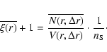
4.3 Conditional average number of galaxies in spheres
In Fig. 12 we show the determination of the whole-sample, average conditional number of points in spheres; i.e., Eq. (5). Given that the PDF in all samples are statistically stable; i.e., they do not show important systematic differences in different sub-volumes, the full
sample volume average provides a meaningful statistical quantity. These behaviors are the same as the ones found by Vasilyev et al. (2006) for the average conditional density. We find that
in all samples,

with
![\begin{figure}
\par\includegraphics*[angle=0, width=8.8cm]{0575Fig8.eps}
\end{figure}](/articles/aa/full_html/2009/10/aa10575-08/img89.gif) |
Figure 8: The same as in Fig. 7 for the sample NGC550 with r=10,15 Mpc/h. For r=15 Mpc/h there are only 3765 determinations. |
| Open with DEXTER | |
![\begin{figure}
\par\includegraphics*[angle=0, width=8.7cm]{0575Fig9.eps}
\end{figure}](/articles/aa/full_html/2009/10/aa10575-08/img90.gif) |
Figure 9: The same as in Fig. 7 for the sample SGC400 with r=5,10,20 Mpc/h. |
| Open with DEXTER | |
![\begin{figure}
\par\includegraphics*[angle=0, width=8.7cm]{0575Fig10.eps}
\end{figure}](/articles/aa/full_html/2009/10/aa10575-08/img91.gif) |
Figure 10: The same as in Fig. 7 for the sample SGC550 with r=10, 20 Mpc/h. |
| Open with DEXTER | |
![\begin{figure}
\par\includegraphics*[angle=0, width=8.7cm]{0575Fig11.eps}
\end{figure}](/articles/aa/full_html/2009/10/aa10575-08/img92.gif) |
Figure 11: Collapse plot of the f(N,r) in the various samples and for the different sphere radius considered. The normalization of the different samples has been performed in an arbitrary way and on the X-axis there are arbitrary units. |
| Open with DEXTER | |
To briefly discuss the determination of the constant pre-factor B in
Eq. (12) (Gabrielli et al. 2005; Joyce & Sylos Labini 2001) and the normalization of the
conditional average density in different VL samples one should
consider the joint conditional probability of finding a galaxy of
luminosity L at distance ![]() from another galaxy; i.e., the
(ensemble) conditional average number of galaxies
from another galaxy; i.e., the
(ensemble) conditional average number of galaxies
![]() with luminosity in the range
with luminosity in the range
![]() and in the volume element
and in the volume element
![]() at distance r from an observer located on a galaxy. We can make the greatly simplifying assumption that
at distance r from an observer located on a galaxy. We can make the greatly simplifying assumption that
where
Using Eq. (13) we may write the conditional average number of galaxies as a function of distance (in case
![]() .)
.)
where N(r;L1VL<L<L2VL) is the number of galaxies in a sphere of radius r and with intrinsic luminosity in the range [L1VL,L2VL], and BVL is the amplitude of the number counts in the VL sample with these limits in absolute luminosity. Because the luminosity function has an exponential cut-off at L*, VL samples containing brighter galaxies show a smaller BVL. By knowing the shape of the luminosity function, it is simple to normalize the different BVL in different VL samples (Joyce & Sylos Labini 2001).
![\begin{figure}
\par\includegraphics*[angle=0, width=8.7cm]{0575Fig12.eps}
\end{figure}](/articles/aa/full_html/2009/10/aa10575-08/img106.gif) |
Figure 12: Average number of points in spheres of radius r around a galaxy. The difference amplitude in samples with different limits in absolute magnitude is simply ascribed by the effect of the luminosity function (see text). Error bars are estimated by the sample dispersion on the average value. |
| Open with DEXTER | |
![\begin{figure}
\par\includegraphics*[angle=0, width=8.7cm]{0575Fig13.eps}
\end{figure}](/articles/aa/full_html/2009/10/aa10575-08/img107.gif) |
Figure 13: The same as in Fig. 12 but divided by the best-fit power-law behavior r2.25. The variation in the amplitude B in Eq. (12) is clearer in this representation. The determination for r>20 Mpc/h is subject to systematic fluctuations, due to the limited volume and the weaker statistics. |
| Open with DEXTER | |
![\begin{figure}
\par\includegraphics*[angle=0, width=8.7cm]{0575Fig14.eps}
\end{figure}](/articles/aa/full_html/2009/10/aa10575-08/img108.gif) |
Figure 14:
Behavior of Eq. (15) with r=5 Mpc/h for NGC400
and SGC400 and
|
| Open with DEXTER | |
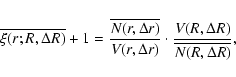
4.4 Average in radial bins
We can now use the data obtained by the SL method to investigate whether there is a convergence to homogeneity on some large scales
![]() Mpc/h; i.e., the largest sphere radius allowed by the geometry of the samples. This is done as follows. We divide the whole range of radial distances in bins of thickness
Mpc/h; i.e., the largest sphere radius allowed by the geometry of the samples. This is done as follows. We divide the whole range of radial distances in bins of thickness ![]() and compute the average
and compute the average
![\begin{displaymath}
\overline{N(r;R,\Delta R)}
= \frac{1}{M_b}
\sum_{R_j\in [R,\Delta R] }^{j=1,M_b} N(r; R_j),
\end{displaymath}](/articles/aa/full_html/2009/10/aa10575-08/img110.gif)
where the sum is extended to the Mb determinations of N(r;R), such that the radial distance is in the interval range
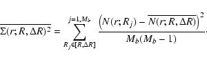
The error analysis in Eq. (16) assumes that the N(r; Rj) are independent, but in fact they are correlated. The errors on these points are therefore substantially under-estimated. However if there is a trend toward homogenization, the error caused by neglecting this correlation will be smaller hence the under estimate of the error bars. Only for the case of a highly correlated distribution does Eq. (16) underestimate the error bars, which than represent a lower limit of the ``true'' error bars.
The quantity given by Eq. (15) and its error (Eq. (16))
provide an estimation of the number of points in spheres of radius r
averaged in thickness bin ![]() .
We expect that, if the distribution converges to uniformity on a scale
.
We expect that, if the distribution converges to uniformity on a scale ![]() ,
then correspondingly
,
then correspondingly
![]() does not
show large fluctuations as a function of R.
does not
show large fluctuations as a function of R.
Results for the four samples are shown in Figs. 14-15. One may note that, for the largest radial bin chosen
![]() Mpc/h, there is no trend
in homogenization, but instead the measurements in bins centered on different R wildly scatters; i.e., their values are outside the statistical error bars given by Eq. (16). This shows that large-scale structures have an amplitude that is incompatible with homogeneity on scales smaller than
Mpc/h, there is no trend
in homogenization, but instead the measurements in bins centered on different R wildly scatters; i.e., their values are outside the statistical error bars given by Eq. (16). This shows that large-scale structures have an amplitude that is incompatible with homogeneity on scales smaller than
![]() Mpc/h.
Mpc/h.
![\begin{figure}
\par\includegraphics*[angle=0, width=9cm]{0575Fig15.eps}\end{figure}](/articles/aa/full_html/2009/10/aa10575-08/img115.gif) |
Figure 15:
As in Fig. 14 but for NGC550 and SGC550 with
r=10 Mpc/h and
|
| Open with DEXTER | |
It is interesting to note that the large fluctuations between the NGC and SGC samples cannot be generated by some redshift-dependent effect, such as the inclusion of galaxy evolution in the computation of absolute magnitudes. Indeed, such a correction, which is expected to be small anyway, given that the redshifts involved do not exceed 0.2, would affect both samples in the same way. Thus by comparing the estimation of the density in bins in the same range of radial distances, we can conclude that the fluctuations we have detected are intrinsic to the distribution of galaxies in these samples. A similar argument can be made for the effect of different cosmologies in the computation of the metric distance.
4.5 Radial counts in VL samples
A complementary way to study fluctuations on large scales in galaxy
redshift surveys is represented by the determination of the radial
counts; i.e., the counts of galaxies as a function of the radial
distance in VL samples (Gabrielli & Sylos Labini 2001). In order to have a statistical
estimator and to evaluate fluctuations, we divided the angular area of
the samples into
![]() non overlapping sub fields of equal solid
angle. For each we compute the differential radial density
non overlapping sub fields of equal solid
angle. For each we compute the differential radial density
![]() in bins of thickness
in bins of thickness
![]() Mpc/h, where ith labels the sub field and R is, as usual, the radial distance. We then can compute the average
Mpc/h, where ith labels the sub field and R is, as usual, the radial distance. We then can compute the average
and the sample variance
Results are shown in Figs. 16-17.
![\begin{figure}
\par\includegraphics*[angle=0, width=9cm]{0575Fig16.eps}
\end{figure}](/articles/aa/full_html/2009/10/aa10575-08/img121.gif) |
Figure 16:
The average differential radial density
|
| Open with DEXTER | |
![\begin{figure}
\par\includegraphics*[angle=0, width=9cm]{0575Fig17.eps}
\end{figure}](/articles/aa/full_html/2009/10/aa10575-08/img122.gif) |
Figure 17: The same as in Fig. 16 for SGC550 and NGC550. |
| Open with DEXTER | |
In the NGC400 sample the structure at 250 Mpc/h is visible as a
relatively large fluctuation of
![]() and a
correspondingly large error. This means that this structure partially
covers the angular area of the survey. In the NGC550 sample, the
radial density is flatter, although there is a large dispersion. In
the SGC400 sample, the structures at 160 Mpc/h and 320 Mpc/h are
identified as local enhancements of
and a
correspondingly large error. This means that this structure partially
covers the angular area of the survey. In the NGC550 sample, the
radial density is flatter, although there is a large dispersion. In
the SGC400 sample, the structures at 160 Mpc/h and 320 Mpc/h are
identified as local enhancements of
![]() .
The
same occurs for the SGC550 case, where the same two structures are
visible. By comparing Figs. 16-17 with
Figs. 1-4 one may note that the SL
analysis is a much more powerful method than the simple counting as a
function of radial distance in tracing large-scale galaxy structures.
.
The
same occurs for the SGC550 case, where the same two structures are
visible. By comparing Figs. 16-17 with
Figs. 1-4 one may note that the SL
analysis is a much more powerful method than the simple counting as a
function of radial distance in tracing large-scale galaxy structures.
4.6 Redshift distribution in the magnitude limit sample
By studying the redshift distribution in the Durham/UKST Galaxy
Redshift Survey, fluctuations have been found in the observed radial
density function are close to 50% occurring on ![]() 50 Mpc/h
scales (Ratcliffe et al. 1998; Busswell et al. 2004). In a similar way in the 2dFGRS
(Busswell et al. 2004), two clear ``holes'' in the galaxy distribution
were detected in the ranges
0.03<z<0.055, with an under-density of
50 Mpc/h
scales (Ratcliffe et al. 1998; Busswell et al. 2004). In a similar way in the 2dFGRS
(Busswell et al. 2004), two clear ``holes'' in the galaxy distribution
were detected in the ranges
0.03<z<0.055, with an under-density of
![]() 40%, and
0.06<z<0.1 where the density deficiency is
40%, and
0.06<z<0.1 where the density deficiency is ![]() 25%. These two under-densities, detected in particular in the 2dFGRS southern galactic cap (SGC), are also clear features in the
Durham/UKST survey. Given that the 2dFGRS SGC field is entirely contained within the areas of sky observed for the Durham/UKST survey, the similarities in the redshift distributions are both proofs of the same features in the galaxy distribution (Busswell et al. 2004).
25%. These two under-densities, detected in particular in the 2dFGRS southern galactic cap (SGC), are also clear features in the
Durham/UKST survey. Given that the 2dFGRS SGC field is entirely contained within the areas of sky observed for the Durham/UKST survey, the similarities in the redshift distributions are both proofs of the same features in the galaxy distribution (Busswell et al. 2004).
We can now compare the redshift distribution in the magnitude limit sample with the results obtained by the SL analysis. In Fig. 18 we report the counting of galaxies as a function of the radial distance, in bins of thickness 10 Mpc/h, in the whole magnitude limited samples. It is interesting to compare these behaviors with Figs. 1-4. The SL method clearly identifies the same structures, which are visible in Fig. 18 as peaks of the radial distribution. However the SL method is able to quantify the amplitude of these fluctuations and, by applying the statistical analysis presented above, to determine how typical these structures are.
![\begin{figure}
\par\includegraphics*[angle=0, width=9cm]{0575Fig18.eps}
\end{figure}](/articles/aa/full_html/2009/10/aa10575-08/img123.gif) |
Figure 18:
Upper panel: radial density in bins of thickness 10 Mpc/h in the NGC magnitude limited sample. The most prominent features identified by the N(r;R) analysis are also visible by the simple counting. There is a large structure at |
| Open with DEXTER | |
4.7 Magnitude counts
In Fig. 19 we report the differential counts of
galaxies as a function of apparent magnitude in the SGC and NGC. The
behaviors are similar to those found by Busswell et al. (2004); Norberg et al. (2002a):
the former paper concluded that there is conclusive evidence that
counts in the SGC are down by 30% relative to the NGC counts. We
find the same difference and, as discussed, we can directly relate it
to the large-scale structures present in both samples. Indeed, as already discussed, the amplitude of the conditional number of galaxies (i.e., Eq. (12)) is ![]()
![]() higher for the NGC samples than for the SGC ones. In other words, in the NGC samples there are more structures, hence fluctuations in the N(r;R), than in SGC samples, as can be seen by
comparing, for instance, Figs. 1-3.
higher for the NGC samples than for the SGC ones. In other words, in the NGC samples there are more structures, hence fluctuations in the N(r;R), than in SGC samples, as can be seen by
comparing, for instance, Figs. 1-3.
![\begin{figure}
\par\includegraphics*[angle=0, width=9cm]{0575Fig19.eps}
\end{figure}](/articles/aa/full_html/2009/10/aa10575-08/img125.gif) |
Figure 19:
Differential counts of galaxies, in bins of
|
| Open with DEXTER | |
4.8 The two-point correlation function
The standard way to measure two-point correlations is accomplished by
determining the function ![]() given by Eq. (11) - see e.g.,
Totsuji & Kihara (1969), Davis & Peebles (1983), Park et al. (1994), Benoist et al. (1996), (), Zehavi et al. (2004), Norberg et al. (2001), Norberg et al. (2002b). As already
mentioned when measuring this quantity it is implicitly assumed that
the distribution is homogeneous well inside the sample volume;
i.e.,
given by Eq. (11) - see e.g.,
Totsuji & Kihara (1969), Davis & Peebles (1983), Park et al. (1994), Benoist et al. (1996), (), Zehavi et al. (2004), Norberg et al. (2001), Norberg et al. (2002b). As already
mentioned when measuring this quantity it is implicitly assumed that
the distribution is homogeneous well inside the sample volume;
i.e.,
![]() .
Let us see what happens when, inside a
spherical sample of radius
.
Let us see what happens when, inside a
spherical sample of radius ![]() there is a fractal distribution with
dimension D<3. We may estimate the sample density
there is a fractal distribution with
dimension D<3. We may estimate the sample density ![]() (which is
not an average quantity) by
(which is
not an average quantity) by
where, in the second equality on the rhs, we used Eq. (12) for the number of points in spheres. Equation (19) shows that the sample density depends on the sample size when D<3. The estimator of the two-point correlation function can be written as (Gabrielli et al. 2005)
The first ratio in the rhs of Eq. (20) is the average conditional density; i.e., the number of galaxies in shells of thickness
which shows that the amplitude of
Equation (21) has been obtained by making the assumption
that the estimation of the sample density is given by the second
equality in the rhs of Eq. (19). This is generallyot the
case, as the sample density in inhomogeneous distributions is subjected to fluctuations of order one on the scale of the sample size. Thus the behavior given by Eq. (21) should be interpreted as giving a very rough estimation of the amplitude of
![]() in a finite sample when there is a fractal distribution inside it.
in a finite sample when there is a fractal distribution inside it.
It is worth noticing that, if the conditional density is a power-law
function of scale, then
![]() is not a power-law
over the same of scales of the conditional density, and particularly
it does not have the same power law index . Indeed, as shown by
Eq. (21),
is not a power-law
over the same of scales of the conditional density, and particularly
it does not have the same power law index . Indeed, as shown by
Eq. (21),
![]() has a a break of the power law
and it is possible to compute analytically the exponent of
has a a break of the power law
and it is possible to compute analytically the exponent of
![]() as a function of the exponent of the conditional
density and the scale ratio
as a function of the exponent of the conditional
density and the scale ratio
![]() (Gabrielli et al. 2005). It is easy to show
that on scales
(Gabrielli et al. 2005). It is easy to show
that on scales
![]() the correlation exponent measured by the
two-point correlation analysis coincides with what is measured by the
conditional density, while on larger scales the exponent measured by
the
the correlation exponent measured by the
two-point correlation analysis coincides with what is measured by the
conditional density, while on larger scales the exponent measured by
the ![]() analysis is generally smaller than D-3. This is indeed
the result obtained by Hawkins et al. (2003, see their Fig. 6).
analysis is generally smaller than D-3. This is indeed
the result obtained by Hawkins et al. (2003, see their Fig. 6).
Let us now evaluate the sample density simply as
![]() in SGC400 and NGC400. Given that the sample geometry is a sphere portion, the volume is given by
in SGC400 and NGC400. Given that the sample geometry is a sphere portion, the volume is given by
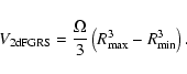 |
(23) |
By using the parameters of the VL samples (see Table 1) we obtain respectively in the SGC400 sample
galaxies per (Mpc/h)3 and in the NGC400 sample
Thus there is a
![\begin{figure}
\par\includegraphics*[angle=0, width=9cm]{0575Fig20.eps}
\end{figure}](/articles/aa/full_html/2009/10/aa10575-08/img141.gif) |
Figure 20: Standard two-point correlation function in the SGC400 and NGC400 sample estimated by Eq. (20). The sample density is simply computed as N/V. |
| Open with DEXTER | |
Different estimators of the two-point correlation function, such as
the Davis and Peebles (DP) (Davis & Peebles 1983) estimator and the Landy and
Szalay (LS) (Landy & Szalay 1993) estimator (see discussion in
Sylos Labini & Vasilyev (2008) for more details about the different estimators),
lead to an estimation of the amplitude of
![]() ,
which
agrees with the one just discussed above. For instance in Fig. 21 a comparison is shown of the different estimators. It is worth noticing that the different estimators give the sample amplitude of
,
which
agrees with the one just discussed above. For instance in Fig. 21 a comparison is shown of the different estimators. It is worth noticing that the different estimators give the sample amplitude of
![]() ,
but they differ in the scale at which
,
but they differ in the scale at which
![]() has the break in the power-law behavior. This is explained by the different ways the estimators treat the boundary conditions, and, particularly, include (implicitly) the global condition known as integral constraint - see discussion in Sylos Labini & Vasilyev (2008).
has the break in the power-law behavior. This is explained by the different ways the estimators treat the boundary conditions, and, particularly, include (implicitly) the global condition known as integral constraint - see discussion in Sylos Labini & Vasilyev (2008).
![\begin{figure}
\par\includegraphics*[angle=0, width=9cm]{0575Fig21.eps}
\end{figure}](/articles/aa/full_html/2009/10/aa10575-08/img142.gif) |
Figure 21: Standard two-point correlation function in the SGC400 measured by means of different estimators, namely the full-shell (FS), the Davis and Peebles (DP) and the Landy and Szalay (LS). |
| Open with DEXTER | |
The sample density ![]() can be estimated differently from Eq. (19). The only condition that it is required for Eq. (20) to be a valid estimator is that the size r* of the
volume entering in the denominator of Eq. (19) be larger than the homogeneity scale
can be estimated differently from Eq. (19). The only condition that it is required for Eq. (20) to be a valid estimator is that the size r* of the
volume entering in the denominator of Eq. (19) be larger than the homogeneity scale ![]() .
In fact, when
.
In fact, when
![]() the estimation of the sample density does not differ substantially from its ensemble average value because, in this
situation, the amplitude of the two-point correlation is, by definition, much smaller than unity. Thus we may consider another estimator of the two-point correlation function, which is the one
introduced by Sylos Labini et al. (2008)
the estimation of the sample density does not differ substantially from its ensemble average value because, in this
situation, the amplitude of the two-point correlation is, by definition, much smaller than unity. Thus we may consider another estimator of the two-point correlation function, which is the one
introduced by Sylos Labini et al. (2008)
where the second ratio on the rhs is the density of points in a shell of thickness
In summary, even though the fact that there is a relatively large
difference in the densities between the NGC and the SGC, the amplitude
of the correlation function is similar because it is measured with
respect to a varying density; i.e., its value reflects the assumption
of homogeneity which is used in the definition in the ![]() -analysis.
Only by analyzing fluctuations that are not normalized to the sample
density one can detect the effect of the large spatial inhomogeneities
characterizing these galaxy samples.
-analysis.
Only by analyzing fluctuations that are not normalized to the sample
density one can detect the effect of the large spatial inhomogeneities
characterizing these galaxy samples.
![\begin{figure}
\par\includegraphics*[angle=0, width=9cm]{0575Fig22.eps}
\end{figure}](/articles/aa/full_html/2009/10/aa10575-08/img150.gif) |
Figure 22:
Standard two-point correlation function in the SGC550 and
NGC550 samples estimated by Eq. (23). The sample average
density is computed in spheres of radius r* and considering all
center points lying in a bin of thickness |
| Open with DEXTER | |
4.9 Analysis in the catalog with conservative cuts in apparent magnitude
We now briefly discuss the results of the SL analysis for the VL samples obtained with conservative magnitude cuts (see Table 2). In Fig. 23 we show the results of the SL analysis: by comparing this figure with Figs. 1-4 by a simple visual inspection one note that structures are extremely similar. Clearly, because of the fewer points contained in the conservative-cuts samples, the value of N(r;R) is different. The behavior of the PDF for the various samples is shown in Fig. 23. The results are thus statistically stable.
![\begin{figure}
\par\includegraphics*[angle=0, width=9cm]{0575Fig23-NEW.eps}
\end{figure}](/articles/aa/full_html/2009/10/aa10575-08/img151.gif) |
Figure 23: SL analysis for the samples with conservative apparent magnitude cuts. The value of the sphere radius is reported in the captions. |
| Open with DEXTER | |
![\begin{figure}
\par\includegraphics*[angle=0, width=9cm]{0575Fig24.eps}
\end{figure}](/articles/aa/full_html/2009/10/aa10575-08/img152.gif) |
Figure 24: PDF of the samples with conservative apparent magnitude cuts. The value of the sphere radius is reported in the labels. In the comparison we used the normalized variable z, by using the transformation described by Eqs. (26)-(27). |
| Open with DEXTER | |
5 Comparison with mock-catalogs
Standard theories of galaxy formation assume that fluctuations in the matter density field in the early universe have very small amplitude, (Peacock 1999; Peebles 1980). In this situation, by denoting as P(k,t), the PS of matter at an arbitrary time ![]() ,
where t=t* corresponds
to some early times in the universe as we discuss below, the prediction of standard cosmological models can be written in this form
,
where t=t* corresponds
to some early times in the universe as we discuss below, the prediction of standard cosmological models can be written in this form
It is possible to write
Gravitational clustering in the linear regime, in an Einstein de
Sitter cosmology, is characterized by a growing and a decaying mode,
both of them power laws in time (Peebles 1980)
![]() .
The amplitude A in Eq. (24) is determined from the
observations of CMBR anisotropies and from the theoretical assumptions
on the nature of cosmological dark matter. From the time dependence
of P(k,t), it is possible to derive the time dependence of
.
The amplitude A in Eq. (24) is determined from the
observations of CMBR anisotropies and from the theoretical assumptions
on the nature of cosmological dark matter. From the time dependence
of P(k,t), it is possible to derive the time dependence of
![]() ,
defined to be
,
defined to be
![]() .
This
grows as a power-law function of time as well: particularly for
power-law PS; i.e.,
.
This
grows as a power-law function of time as well: particularly for
power-law PS; i.e.,
![]() and n<4, one obtains
(Peebles 1980)
and n<4, one obtains
(Peebles 1980)
 |
(26) |
To summarize the situation, we may identify two length-scales at the present time. The first is the homogeneity (or nonlinearity) scale
In order to study gravitational structure formation in the nonlinear phase, the common practice is to perform N-body simulations of theoretical models. This is done by integrating the equation of motions of N self-gravitating particles, in a volume V and by making use of periodic boundary conditions to represent an infinite (periodic) system. Initial particle correlations are given according to a given theoretical model, and the initial redshift is generally z>10. The simulation is then run up to z=0. In addition the space background is expanding and thus one follows the particles' motion in comoving coordinates. Particles are supposed to simulate the motion of fluid elements of the underlying dark matter field.
To identify galaxies one uses a phenomenological approach. As discussed, galaxies are supposed to form in the highest density peaks of the dark matter field. Thus when the simulation has reached the redshift z=0, one uses semi-analytic models to identify galaxies. Among the largest simulations made publicy available, the millennium run (Springel et al. 2005) used more than 10 billion particles to trace the evolution of the matter distribution in a region of the universe in a cubic box of 500 Mpc/h. Semi-analytic catalogs constructed from the millennium run contains about 10 million objects (Croton et al. 2006).
Here we analyze the semi-analytic catalog containing 9 925 229 objects
in which the absolute magnitudes of mock-galaxies are given in the
BVRIK filters. To reproduce the same limits in absolute magnitude of
the volume-limited samples of the 2dFGRS, we used the relations
between magnitude in different filters given by Colless et al. (2001). In
this way we selected respectively 1 119 434 and 368 619 galaxies in a
500 Mpc/h cube. We then selected three slices with the same geometry
of the real 2dFGRS samples, which are hereafter called SGC400m,
NGC400m and NGC550m. The remaining sample, SGC550m, is ![]() wide instead of
wide instead of ![]() as in real data. The number of objects in
each of the four samples is close to the one in the corresponding real
2dFGRS sample.
as in real data. The number of objects in
each of the four samples is close to the one in the corresponding real
2dFGRS sample.
In Fig. 25 we show the behavior of the SL analysis for the
mock-sample SGC550m in real and redshift space for r=20 Mpc/h (see
for comparison Figs. 2-4). The
effect of peculiar velocities is that of enhancing a little the
structures that appear in real space. That the difference between
real and redshift space is small for sphere radius ![]() Mpc/h is
shown in Figs. 26-27, where we plot the PDF
of conditional fluctuations. In this case we used the normalized
variable
Mpc/h is
shown in Figs. 26-27, where we plot the PDF
of conditional fluctuations. In this case we used the normalized
variable
and we thus determine its PDF, that is,
where f(N,r) is the PDF of the variable Ni(r),
![\begin{figure}\par\includegraphics*[angle=0, width=9cm]{0575Fig25-NEW.eps}\par\end{figure}](/articles/aa/full_html/2009/10/aa10575-08/img179.gif) |
Figure 25: SL analysis with sphere radius r=20 Mpc/h, for the mock-sample SGC550m (the samples with better statistics) in real space ( upper panel) and in redshift space ( bottom panel). |
| Open with DEXTER | |
![\begin{figure}\par\includegraphics*[angle=0, width=9cm]{0575Fig26.eps}\par\end{figure}](/articles/aa/full_html/2009/10/aa10575-08/img180.gif) |
Figure 26: PDF for the mock-samples SGC400m and NGC400m in real space (RS) and redshift space (ZS) for r=10 Mpc/h. The best fit with a Gaussian function is reported as reference. |
| Open with DEXTER | |
![\begin{figure}\par\includegraphics*[angle=0, width=9cm]{0575Fig27.eps}\par\end{figure}](/articles/aa/full_html/2009/10/aa10575-08/img181.gif) |
Figure 27: The same as in Fig. 26 but for the case r=20 Mpc/h and for the mock-samples SGC550m and NGC500m. |
| Open with DEXTER | |
In Figs. 28-29 we show the comparison between the PDF in the mock-sample SGC500m (redshift space) and the one in the real sample SGC550. Both for the sphere radius r=10 Mpc/h and r=20 Mpc/h, fluctuations are more persistent in real samples than in mock-samples and this is reflected in the relatively fat tail of the PDF for large N values.
![\begin{figure}
\par\includegraphics*[angle=0, width=9cm]{0575Fig28.eps}
\end{figure}](/articles/aa/full_html/2009/10/aa10575-08/img182.gif) |
Figure 28: Comparison between the PDF in the mock-sample SGC400m (redshift space) and the one in the real sample SGC400. Poisson error bars are displayed as a reference. |
| Open with DEXTER | |
![\begin{figure}
\par\includegraphics*[angle=0, width=9cm]{0575Fig29.eps}
\end{figure}](/articles/aa/full_html/2009/10/aa10575-08/img183.gif) |
Figure 29: The same as in Fig. 28 but for the case r=20 Mpc/h and for the sample SGC550. |
| Open with DEXTER | |
In Fig. 30 (upper panel) it is shown the behavior of
the whole-sample average number of points is spheres;
i.e., Eq. (5). For
![]() Mpc/h, the function
Mpc/h, the function
![]() growths with an exponent equal to the space
dimension (i.e., D=3). On smaller scales the exponent is instead
growths with an exponent equal to the space
dimension (i.e., D=3). On smaller scales the exponent is instead
![]() .
.
![\begin{figure}
\par\includegraphics*[angle=0, width=9cm]{0575Fig30.eps}
\end{figure}](/articles/aa/full_html/2009/10/aa10575-08/img186.gif) |
Figure 30:
Upper panel: whole-sample average number of points in
spheres; i.e., Eq. (5) for the mock-samples in real space.
Bottom panel: behavior of Eq. (15) for the mock-galaxy
samples in real space for SGC550m; the sphere radius is r=10 Mpc/h
and the radial bin thickness is
|
| Open with DEXTER | |
Finally in the Fig. 30 (bottom panel) the behavior of
of Eq. (15) with r=5 Mpc/h is shown for the mock-galaxy
samples in real space. Fluctuations, when averaged over radial bin of
thickness
![]() Mpc/h are more smooth and quiet than the real
samples and thus that there are no large fluctuations on scales larger
than
Mpc/h are more smooth and quiet than the real
samples and thus that there are no large fluctuations on scales larger
than
![]() .
This is clearly consistent with the behavior of
the PDF described previously. The small difference for small R is
due to the lower statistics at the nearby boundary of the samples.
.
This is clearly consistent with the behavior of
the PDF described previously. The small difference for small R is
due to the lower statistics at the nearby boundary of the samples.
Because the distribution becomes uniform at scales
![]() Mpc/h, the two-point correlation function is well-defined, both in
real and redshift space. This presents an intrinsic length scale
Mpc/h, the two-point correlation function is well-defined, both in
real and redshift space. This presents an intrinsic length scale
![]() at about
at about
![]() Mpc/h, and beyond that scale it
rapidly decays to zero.
Mpc/h, and beyond that scale it
rapidly decays to zero.
The whole-sample average number of points in spheres
(i.e., Eq. (5)) does show a systematic difference with respect to
the real-space case. Indeed, while for
![]() Mpc/h it
again shows a power-law behavior with D=3, on smaller scales the
exponent is
Mpc/h it
again shows a power-law behavior with D=3, on smaller scales the
exponent is
![]() instead of D=1.2 as for the real space
case (see Fig. 31 -- upper panel). In addition,
the transition between the two regimes is faster than for the real
space case.
instead of D=1.2 as for the real space
case (see Fig. 31 -- upper panel). In addition,
the transition between the two regimes is faster than for the real
space case.
![\begin{figure}
\par\includegraphics*[angle=0, width=9cm]{0575Fig31.eps}
\end{figure}](/articles/aa/full_html/2009/10/aa10575-08/img190.gif) |
Figure 31:
Upper panel: whole-sample average number of points in
spheres; i.e., Eq. (5). for the mock-samples in redshift space.
Bottom panel: behavior of Eq. (15) for the mock-samples
in redshift space for SGC550m; the sphere radius is r=10 Mpc/h and
the radial bin thickness is
|
| Open with DEXTER | |
Finally in Fig. 31 (bottom panel) the behavior of
Eq. (15) is reported for the mock-samples in redshift space. As
for the real-space case, and consistent with the behaviors of the PDF
in redshift space, fluctuations are substantially smoothed when
averaged over radial bins of size
![]() .
.
6 Discussion and conclusions
We characterized fluctuations and correlations in the galaxy distribution, by considering several samples from the 2dFGRS (Colless et al. 2001). The main point of our analysis is to use statistical quantities that measure fluctuations amplitude not normalizing it to the sample average. Our main results are:
- Estimations of the sample average are affected by systematic
variations that are the imprint of the structures with the large
spatial extension present in these samples, which correspond to
large amplitude fluctuations. To identify structures in redshift
space we applied the scale-length (SL) method, introduced in
Sylos Labini et al. (2008).
- The probability density function (PDF) of conditional
fluctuations is, in all considered samples and up to r=20 Mpc/h
(the largest distance scale we considered for this statistics),
wildly different from a Gaussian function and characterized by a
long tail, possibly with a power-law decay, signaling the presence
of large fluctuations (e.g. structures) in the density field. These
fluctuations are persistent up to scales limited by sample sizes.
- The first moment of the PDF shows scaling properties, that
correspond to a fractal dimension
 up to
up to
 Mpc/h. At the largest distance scale we considered; i.e., for
r>20 Mpc/h, determinations are affected by relatively large
fluctuations that reflect the intrinsic systematic error induced by
structures, and thus the results have weaker statistical
significance for the limited volume and number of points
contributing to the average. This agrees with our previous findings
in Vasilyev et al. (2006).
Mpc/h. At the largest distance scale we considered; i.e., for
r>20 Mpc/h, determinations are affected by relatively large
fluctuations that reflect the intrinsic systematic error induced by
structures, and thus the results have weaker statistical
significance for the limited volume and number of points
contributing to the average. This agrees with our previous findings
in Vasilyev et al. (2006).
- The homogeneity scale, i.e. the scale beyond which fluctuations
become small and the sample density estimation approaches the value
of the (ensemble) average density, has a lower limit at
 Mpc/h. This is because fluctuations on scales of about 70 Mpc/h
are incompatible with a transition to homogeneity on that scale.
This result is consistent with the results by
Ratcliffe et al. (1998); Busswell et al. (2004). The main results obtained in this
survey are in very good agreement with a similar analysis of galaxy
samples extracted from the SDSS (Sylos Labini et al. 2008).
Mpc/h. This is because fluctuations on scales of about 70 Mpc/h
are incompatible with a transition to homogeneity on that scale.
This result is consistent with the results by
Ratcliffe et al. (1998); Busswell et al. (2004). The main results obtained in this
survey are in very good agreement with a similar analysis of galaxy
samples extracted from the SDSS (Sylos Labini et al. 2008).
- The SL method is suitable and effective in tracing structures in
redshift space and in measuring the amplitude and distribution of
density fluctuations. Galaxy counts results can be easily related
to the results obtained by the SL method. Indeed we confirmed that
the variation of about
 30% between galaxy counts as a
function of apparent magnitude in the northern and southern angular
regions of this survey, detected by Busswell et al. (2004), can be
easily related to the different structures present in the different
samples. Moreover, such large fluctuations, make any estimation of
the sample average, on comparable scales to the samples sizes,
affected by strong systematic effects.
30% between galaxy counts as a
function of apparent magnitude in the northern and southern angular
regions of this survey, detected by Busswell et al. (2004), can be
easily related to the different structures present in the different
samples. Moreover, such large fluctuations, make any estimation of
the sample average, on comparable scales to the samples sizes,
affected by strong systematic effects.
- Apparently the amplitude the two-point correlation function,
which normalizes the amplitude of fluctuations (as a function of
scale) to the estimation of the sample average, of is not affected
by fluctuations, and that this is stable in the Northern and
Southern samples. This occurs, however, because of the
normalization to the sample average (i.e., the denominator of
 )
which indeed shows the same large variation between the
two angular regions as the conditional density (i.e., the nominator
of ). Thus the normalization of fluctuations amplitude to
the sample average hides the presence of large differences between
the two samples, being biased by uncontrolled systematic
finite-size effects. In this situation the amplitude of the
two-point correlation function does not give a reliable and
meaningful estimation of either the statistical properties of
galaxy distribution in these samples, the spatial extension of
correlations, or of amplitude of fluctuations. It is indeed the
normalization of fluctuations amplitude to a not well defined
quantity, the sample density, which in this case determines the
spurious length scale
)
which indeed shows the same large variation between the
two angular regions as the conditional density (i.e., the nominator
of ). Thus the normalization of fluctuations amplitude to
the sample average hides the presence of large differences between
the two samples, being biased by uncontrolled systematic
finite-size effects. In this situation the amplitude of the
two-point correlation function does not give a reliable and
meaningful estimation of either the statistical properties of
galaxy distribution in these samples, the spatial extension of
correlations, or of amplitude of fluctuations. It is indeed the
normalization of fluctuations amplitude to a not well defined
quantity, the sample density, which in this case determines the
spurious length scale
 Mpc/h.
- We compared the results by studying conditional fluctuations in the 2dFGRS samples with those obtained in mock-galaxy catalogs. These are constructed from the dark matter density field in cosmological simulations which were evolved to study the effect of non-linear gravitational clustering in an expanding universe. We used the mock-galaxy samples provided by Croton et al. (2006) and obtained from the largest N-body simulations publicly available at the moment (Springel et al. 2005). We have studied the mock-galaxy catalogs both in real and redshift space, so to take into account the distortions due to the effect of peculiar velocities. We found that the PDF of conditional fluctuations is weakly affected by peculiar velocities and that it rapidly converges to a Gaussian function on scales r>10 Mpc/h, in agreement with predictions of theoretical models both in real and redshift space. On smaller scales, i.e. r<10 Mpc/h, the PDF presents a longer tail than the Gaussian function. This is the signature of the nonlinear structures formed at small scales. Indeed, the PDF of mock-galaxy catalogs reflect the dynamics that has given rise to structures in the simulations. In this respect, correlations provided by theoretical models and given as initial conditions for the simulations are of CDM type. In these models gravitational clutering forms nonlinear structures (i.e., large fluctuations in the density field) up to the limited range of about 10 Mpc/h. Such a length scale can be easily predicted by considering the initial amplitude of fluctuations in these models, normalized to CMBR anisotropies, and by computing the evolution in an expanding universe of the linear regime of gravitational clustering. Note that Einasto et al. (2006) reached a similar conclusion; i.e., that in the 2dFGRS there are several rich super-clusters which is higher than what is found in similar volumes in the Millennium simulation.
Acknowledgements
We thank Michael Joyce, Andrea Gabrielli, and Luciano Pietronero for useful remarks and discussions. We are grateful to Martin Lopez-Correidoira and Michael Blanton for interesting comments. We also thank an anonymous referee for useful suggestions. Yu.B. thanks the RF grant ``Leading Scientific School'' for partial financial support. We acknowledge the use of the 2dFGRS data available at http://www.mso.anu.edu.au/2dFGRS/ and of the millennium run semi-analytic galaxy catalog available at http://www.mpa-garching.mpg.de/galform/agnpaper/
References
- Baryshev, Yu., & Teerikorpi, P. 2006, Bull. Spec. Astrop. Obs., 59, 92
- Benoist, C., Maurogordato, S., da Costa, L. N., Cappi, A., & Schaeffer, R. 1996, ApJ, 472, 452 [NASA ADS] [CrossRef] (In the text)
- Busswell, G. S., Shanks, T., Frith, W. J., et al., 2004, MNRAS, 354, 991 [NASA ADS] [CrossRef] (In the text)
- Chiaki, H., Schmalzing, J., Buchert, T., et al. 2003, PASJ, 55, 911 [NASA ADS]
- Colless, M., Dalton, G., Maddox, S., et al. 2001, MNRAS, 328, 1039 [NASA ADS] [CrossRef]
- Croton, D. J., Springel, V., White, S. D. M., et al. 2006, MNRAS, 365, 11 [NASA ADS] [CrossRef] (In the text)
- da Costa, L., Pellegrini, P. S., Sargent, W. L. W., et al. 1988, ApJ, 327, 544 [NASA ADS] [CrossRef]
- Davis, M., & Huchra, J. 1982, ApJ, 254, 437 [NASA ADS] [CrossRef] (In the text)
- Davis, M., & Peebles, P. J. E. 1983, ApJ, 267, 465 [NASA ADS] [CrossRef] (In the text)
- Davis, M., Meiksin, A., Strauss, M. A., et al. 1988, ApJ, 333, L9 [NASA ADS] [CrossRef] (In the text)
- de Lapparent, V., Geller, M. J., & Huchra, J. P. 1986, ApJ, 302, 1 [NASA ADS] [CrossRef]
- de Vaucouleurs, G. 1970, Science, 167, 1203 [NASA ADS] [CrossRef] (In the text)
- Durrer, R., Gabrielli, A., Joyce, M., & Sylos Labini, F. 2003, ApJ, 585, L1 [NASA ADS] [CrossRef]
- Eke, V. R., Baugh, C. M., Cole, S., et al. 2004, MNRAS, 348, 866 [NASA ADS] [CrossRef] (In the text)
- Einasto, J., Einasto, M., Saar, E., et al. 2006, A&A, 459, L1 [NASA ADS] [CrossRef] [EDP Sciences] (In the text)
- Falco, E. F., Kurtz, M. J., Geller, M. J., et al. 1999, PASP, 111, 438 [NASA ADS] [CrossRef]
- Frith, W. J., Busswell, G. S., Fong, R., Metcalfe, N., & Shanks, T. 2003, MNRAS, 345, 1049 [NASA ADS] [CrossRef]
- Gabrielli, A., & Sylos Labini, F. 2001, Europhys. Lett., 54, 286 [NASA ADS] [CrossRef] (In the text)
- Gabrielli, A., Joyce, M., & Sylos Labini, F. 2002, Phys. Rev. D, 65, 083523 [NASA ADS] [CrossRef]
- Gabrielli, A., Sylos Labini, F., Joyce, M., & Pietronero, L. 2005 Statistical Physics for Cosmic Structures (Berlin: Springer Verlag)
- Geller, M., & Huchra J. 1989, Science, 246, 897 [NASA ADS] [CrossRef]
- Giovanelli, R., & Haynes, M. P. 1993, AJ, 105, 1271 [NASA ADS] [CrossRef]
- Gott, J., Richard, III, Juric', M., & Schlegel, D. 2005, ApJ, 624, 463 [NASA ADS] [CrossRef]
- Hawkins, Ed, Maddox, S., Cole, S., et al. 2003, MNARS, 346, 78 [CrossRef] (In the text)
- Hogg, D. W., Eisenstein, D., Blanton, M., et al. 2005, ApJ, 624, 54 [NASA ADS] [CrossRef]
- Hogg, D. W., Baldry, I. K., Blanton, M. R., & Eisenstein, D. J. 2002,[arXiv:astro-ph/0210394v1] (In the text)
- Huchra, D., Latham, & Tonry, 1983, ApJS 52, 89 [NASA ADS] [CrossRef]
- Kaiser, N. 1984, ApJ, 284, L9 [NASA ADS] [CrossRef]
- Kerscher, M., Schmalzing, J., Buchert, T., & Wagner, H. 1998, A&A, 333, 1 [NASA ADS]
- Kerscher, M. 1999, A&A, 343, 333 [NASA ADS]
- Joyce, M., & Sylos, L. F. 2001, ApJ, 554, L1 [NASA ADS] [CrossRef]
- Landy, S. D., & Szalay, A. 1993, ApJ, 412, 64 [NASA ADS] [CrossRef] (In the text)
- Madgwick, D. S., Lahav, O., Baldry, I. K., et al. 2002, MNRAS, 333, 133 [NASA ADS] [CrossRef] (In the text)
- Norberg, P., Baugh, C. M., Hawkins, Ed., et al. 2001, MNRAS, 328, 64 [NASA ADS] [CrossRef] (In the text)
- Norberg, P., Cole, S., Baugh, C. M., et al. 2002a, MNRAS, 336, 907 [NASA ADS] [CrossRef]
- Norberg, P., Baugh, C. M., Hawkins, Ed., et al. 2002b, MNRAS, 332, 827 [NASA ADS] [CrossRef]
- Park, C., Vogeley, M. S., Geller, M. J., & Huchra, J. P. 1994, ApJ, 431, 569 [NASA ADS] [CrossRef] (In the text)
- Peacock, J. A. 1999, Cosmological physics (Cambridge University Press) (In the text)
- Peebles, P. J. E. 1980, The Large-Scale Structure of the Universe (Princeton University Press)
- Picard, A. 1991, AJ, 102, 445 [NASA ADS] [CrossRef]
- Ratcliffe, A., Shanks, T., Parker, Q. A., & Fong, R., 1998, MNRAS, 293, 197 [NASA ADS] [CrossRef]
- Saslaw, W. C. 2000, The Distribution of the Galaxies, (Cambridge: Cambridge University Press) (In the text)
- Shectman, S. A., Landy, S. D., Oemler, A. et al. 1996, ApJ, 470, 172 [NASA ADS] [CrossRef]
- Spergel, D. N., Bean, R., Doré, O., et al. 2007, ApJS, 170, 377 [NASA ADS] [CrossRef]
- Springel, V., White, S. D. M., Jenkins, A., et al. 2005, Nature, 435, 629 [NASA ADS] [CrossRef] (In the text)
- Sylos Labini, F., Montuori, M., & Pietronero, L. 1988, Phys. Rep., 293, 61 [NASA ADS] [CrossRef]
- Sylos Labini, F., Vasilyev, N. L., & Baryshev, Yu. V. 2007, A&A, 465, 23 [NASA ADS] [CrossRef] [EDP Sciences]
- Sylos Labini, F., Vasilyev, N. L., Pietronero, L., Baryshev, & Yu. V. 2008, [arXiv:0805.1132v1]
- Sylos Labini, F., & Vasilyev, N. L. 2008, A&A, 477, 381 [NASA ADS] [CrossRef] [EDP Sciences] (In the text)
- Sylos Labini, F., Vasilyev, N. L., & Baryshev, Yu. V. 2009, Europhys. Lett., 85, 29002 [NASA ADS] [CrossRef]
- Torquato, S., & Stillinger, F. H. 2003, Phys. Rev. E, 68, 041113 [NASA ADS] [CrossRef] (In the text)
- Totsuji, H., & Kihara, T. 1969, PASJ, 21, 221 [NASA ADS] (In the text)
- Vasilyev, N. L., Baryshev, Yu. V., & Sylos Labini, F., 2006, A&A, 447, 431 [NASA ADS] [CrossRef] [EDP Sciences]
- York, Donald, G., Adelman, J., Anderson, J. E., Jr., et al. 2000, AJ, 120, 1579 [NASA ADS] [CrossRef]
- Weir, N., Djorgovski, G. S., & Fayyad, U. M. 1995, AJ, 110, 1 [NASA ADS] [CrossRef]
- Wu, K. K., Lahav, O., & Rees, M. 1999, Nature, 225, 230
- Zehavi, I., Blanton, M. R., Frieman, J. A., et al. 2002, ApJ, 571, 172 [NASA ADS] [CrossRef] (In the text)
- Zehavi, I., Weinberg, D. H., Zheng, Z., et al. 2004, ApJ, 608, 16 [NASA ADS] [CrossRef] (In the text)
- Zehavi, I., Eisenstein, D. J., Nichol, R. C., et al. 2005, ApJ, 621, 22 [NASA ADS] [CrossRef]
Footnotes
- ...
homogeneity
![[*]](/icons/foot_motif.gif)
- Note that de Vaucouleurs simply considered the scale where galaxies approaches a random distribution. A distribution can be homogeneous, i.e. with a well-defined mean density, without being random; i.e. there can be small amplitude fluctuations with weak long-range correlations.
- ...
size
- We use
 h km s-1 Mpc-1 for the value of the Hubble constant.
- ... function
- These statistics,
as mentioned above, normalize the amplitude of fluctuations to the
estimation of the sample density. From it the length scale
-8 Mpc/h is derived.
- ... directions
- Because of the hypothesis of statistical stationarity, statistical quantities generally depend only of the scalar distance between points.
- ... uniform
- To avoid confusion a stationary stochastic point process with a positive ensemble average density is sometimes denoted as uniform and nonuniform when this is equal to zero. Both are statistically homogeneous stochastic processes (Gabrielli et al. 2005).
- ...

- See below for a precise definition.
- ... galaxy
- This is thus a conditional quantity.
- ... function
- This is clearly the case if the number of points is large enough, otherwise the PDF is described by the Poisson distribution.
- ... samples
- Note that, for instance, Einasto et al. (2006); Eke et al. (2004) used different methods to identify the same structures we observe.
- ... scale
- Pair-counting based estimators, like the Davis & Peebles and/or the Landy & Szalay estimator, have the same pathologies when the conditional density is a power law as a function of scale (Gabrielli et al. 2005).
All Tables
Table 1:
Main properties of the obtained VL samples. ![]() ,
,
![]() are the chosen limits for the metric distance;
are the chosen limits for the metric distance;
![]() are the corresponding limits in the absolute magnitude;
are the corresponding limits in the absolute magnitude; ![]() is the number of galaxies in the sample.
is the number of galaxies in the sample.
Table 2: As Table 1 but for the case of more conservative cuts in apparent magnitudes; i.e. 14.5<bJ<19.3, were used for selecting the galaxies.
All Figures
| |
Figure 1: From top to bottom the SL analysis for the sample NGC400 with r=5,10 Mpc/h. |
| Open with DEXTER | |
| In the text | |
| |
Figure 2: The same as Fig. 1 but now for the sample NGC550 with r=10,15 Mpc/h. |
| Open with DEXTER | |
| In the text | |
| |
Figure 3: The same as Fig. 1 but now for the sample SGC400 with r=5,10,20 Mpc/h. |
| Open with DEXTER | |
| In the text | |
| |
Figure 4: The same as Fig. 1 but now for the sample SGC550 with r=10,20,30 Mpc/h. |
| Open with DEXTER | |
| In the text | |
| |
Figure 5: The SL analysis for the SGC550 sample. On the X and Y axes the coordinate of the center of a sphere of radius r=10 Mpc/h (centered on a galaxy) is reported and on the Z axis the number of galaxies inside it. The mean thickness of this slice is about 50 Mpc/h. Large fluctuations in the density field traced by the SL analysis are located in the correspondence of large-scale structures. |
| Open with DEXTER | |
| In the text | |
| |
Figure 6: Number of center-points M(r) as a function of the sphere radius r in the various samples considered. |
| Open with DEXTER | |
| In the text | |
| |
Figure 7:
Probability density function f(N,r) of the values
|
| Open with DEXTER | |
| In the text | |
| |
Figure 8: The same as in Fig. 7 for the sample NGC550 with r=10,15 Mpc/h. For r=15 Mpc/h there are only 3765 determinations. |
| Open with DEXTER | |
| In the text | |
| |
Figure 9: The same as in Fig. 7 for the sample SGC400 with r=5,10,20 Mpc/h. |
| Open with DEXTER | |
| In the text | |
| |
Figure 10: The same as in Fig. 7 for the sample SGC550 with r=10, 20 Mpc/h. |
| Open with DEXTER | |
| In the text | |
| |
Figure 11: Collapse plot of the f(N,r) in the various samples and for the different sphere radius considered. The normalization of the different samples has been performed in an arbitrary way and on the X-axis there are arbitrary units. |
| Open with DEXTER | |
| In the text | |
| |
Figure 12: Average number of points in spheres of radius r around a galaxy. The difference amplitude in samples with different limits in absolute magnitude is simply ascribed by the effect of the luminosity function (see text). Error bars are estimated by the sample dispersion on the average value. |
| Open with DEXTER | |
| In the text | |
| |
Figure 13: The same as in Fig. 12 but divided by the best-fit power-law behavior r2.25. The variation in the amplitude B in Eq. (12) is clearer in this representation. The determination for r>20 Mpc/h is subject to systematic fluctuations, due to the limited volume and the weaker statistics. |
| Open with DEXTER | |
| In the text | |
| |
Figure 14:
Behavior of Eq. (15) with r=5 Mpc/h for NGC400
and SGC400 and
|
| Open with DEXTER | |
| In the text | |
| |
Figure 15:
As in Fig. 14 but for NGC550 and SGC550 with
r=10 Mpc/h and
|
| Open with DEXTER | |
| In the text | |
| |
Figure 16:
The average differential radial density
|
| Open with DEXTER | |
| In the text | |
| |
Figure 17: The same as in Fig. 16 for SGC550 and NGC550. |
| Open with DEXTER | |
| In the text | |
| |
Figure 18:
Upper panel: radial density in bins of thickness 10 Mpc/h in the NGC magnitude limited sample. The most prominent features identified by the N(r;R) analysis are also visible by the simple counting. There is a large structure at |
| Open with DEXTER | |
| In the text | |
| |
Figure 19:
Differential counts of galaxies, in bins of
|
| Open with DEXTER | |
| In the text | |
| |
Figure 20: Standard two-point correlation function in the SGC400 and NGC400 sample estimated by Eq. (20). The sample density is simply computed as N/V. |
| Open with DEXTER | |
| In the text | |
| |
Figure 21: Standard two-point correlation function in the SGC400 measured by means of different estimators, namely the full-shell (FS), the Davis and Peebles (DP) and the Landy and Szalay (LS). |
| Open with DEXTER | |
| In the text | |
| |
Figure 22:
Standard two-point correlation function in the SGC550 and
NGC550 samples estimated by Eq. (23). The sample average
density is computed in spheres of radius r* and considering all
center points lying in a bin of thickness |
| Open with DEXTER | |
| In the text | |
| |
Figure 23: SL analysis for the samples with conservative apparent magnitude cuts. The value of the sphere radius is reported in the captions. |
| Open with DEXTER | |
| In the text | |
| |
Figure 24: PDF of the samples with conservative apparent magnitude cuts. The value of the sphere radius is reported in the labels. In the comparison we used the normalized variable z, by using the transformation described by Eqs. (26)-(27). |
| Open with DEXTER | |
| In the text | |
| |
Figure 25: SL analysis with sphere radius r=20 Mpc/h, for the mock-sample SGC550m (the samples with better statistics) in real space ( upper panel) and in redshift space ( bottom panel). |
| Open with DEXTER | |
| In the text | |
| |
Figure 26: PDF for the mock-samples SGC400m and NGC400m in real space (RS) and redshift space (ZS) for r=10 Mpc/h. The best fit with a Gaussian function is reported as reference. |
| Open with DEXTER | |
| In the text | |
| |
Figure 27: The same as in Fig. 26 but for the case r=20 Mpc/h and for the mock-samples SGC550m and NGC500m. |
| Open with DEXTER | |
| In the text | |
| |
Figure 28: Comparison between the PDF in the mock-sample SGC400m (redshift space) and the one in the real sample SGC400. Poisson error bars are displayed as a reference. |
| Open with DEXTER | |
| In the text | |
| |
Figure 29: The same as in Fig. 28 but for the case r=20 Mpc/h and for the sample SGC550. |
| Open with DEXTER | |
| In the text | |
| |
Figure 30:
Upper panel: whole-sample average number of points in
spheres; i.e., Eq. (5) for the mock-samples in real space.
Bottom panel: behavior of Eq. (15) for the mock-galaxy
samples in real space for SGC550m; the sphere radius is r=10 Mpc/h
and the radial bin thickness is
|
| Open with DEXTER | |
| In the text | |
| |
Figure 31:
Upper panel: whole-sample average number of points in
spheres; i.e., Eq. (5). for the mock-samples in redshift space.
Bottom panel: behavior of Eq. (15) for the mock-samples
in redshift space for SGC550m; the sphere radius is r=10 Mpc/h and
the radial bin thickness is
|
| Open with DEXTER | |
| In the text | |
Copyright ESO 2009
Current usage metrics show cumulative count of Article Views (full-text article views including HTML views, PDF and ePub downloads, according to the available data) and Abstracts Views on Vision4Press platform.
Data correspond to usage on the plateform after 2015. The current usage metrics is available 48-96 hours after online publication and is updated daily on week days.
Initial download of the metrics may take a while.