| Issue |
A&A
Volume 494, Number 3, February II 2009
|
|
|---|---|---|
| Page(s) | 867 - 877 | |
| Section | Cosmology (including clusters of galaxies) | |
| DOI | https://doi.org/10.1051/0004-6361:20079184 | |
| Published online | 22 December 2008 | |
The galaxy cross-correlation function as a probe of the spatial distribution of galactic satellites
J. Chen1,2
1 - Argelander-Institut für Astronomie, Universität Bonn,
Auf dem Hügel 71,
53121 Bonn, Germany
2 -
Kavli Institute for Cosmological Physics, Dept. of Astronomy & Astrophysics,
University of Chicago,
5640 South Ellis Avenue,
Chicago, IL 60637, USA
Received 3 December 2007 / Accepted 8 December 2008
Abstract
The spatial distribution of satellite galaxies around host galaxies can illuminate the relationship between satellites and dark matter subhalos and aid in developing and testing galaxy formation models. Previous efforts to constrain the distribution attempted to eliminate interlopers from the measured projected number density of satellites and found that the distribution is generally consistent with the expected dark matter halo profile of the parent hosts, with a best-fit power-law slope of ![]() -1.7 between projected separations of
-1.7 between projected separations of ![]() 30 h-1 kpc and
0.5 h-1 Mpc. Here, I use the projected cross-correlation of bright and faint galaxies to analyze contributions from satellites and interlopers together, using a halo occupation distribution (HOD) analytic model for galaxy clustering. This approach is tested on mock catalogs constructed from simulations. I find that analysis of Sloan Digital Sky Survey (SDSS) data gives results generally consistent with interloper subtraction methods between the projected separations of 10 h-1 kpc and
6.3 h-1 Mpc, although the errors on the parameters that constrain the radial profile are large, and larger samples of data are required.
30 h-1 kpc and
0.5 h-1 Mpc. Here, I use the projected cross-correlation of bright and faint galaxies to analyze contributions from satellites and interlopers together, using a halo occupation distribution (HOD) analytic model for galaxy clustering. This approach is tested on mock catalogs constructed from simulations. I find that analysis of Sloan Digital Sky Survey (SDSS) data gives results generally consistent with interloper subtraction methods between the projected separations of 10 h-1 kpc and
6.3 h-1 Mpc, although the errors on the parameters that constrain the radial profile are large, and larger samples of data are required.
Key words: cosmology: theory - cosmology: dark matter - galaxies: formation - galaxies: structure - galaxies: fundamental parameters
1 Introduction
In the hierarchical assembly of dark matter (DM) halos, progenitor halos merge to form larger systems. Some DM halos survive accretion and form a population of subhalos within the virial radius of the larger halo (e.g., Ghigna et al. 1998; Klypin et al. 1999). Baryonic material cools and forms stars in the center of some halos and subhalos, resulting in galaxies and satellite galaxies. Satellite galaxies are biased tracers of the potential well of their host DM halos, and satellite dynamics have been used to provide constraints on the total mass distribution in galactic halos (e.g., van den Bosch et al. 2004; Zaritsky et al. 1997; Conroy et al. 2005; Prada et al. 2003; Faltenbacher & Diemand 2006; Zaritsky & White 1994) and to test the nature of gravity (Klypin & Prada 2009). In addition, the spatial distribution of the satellite galaxy population reflects the evolution of dwarf galaxies and the mass accretion history of the halo. For example, observations of satellites around early-type galaxies suggest that the distribution lies along the major axis of the light distribution (e.g., Brainerd 2005; Yang et al. 2006; Azzaro et al. 2007; Sales & Lambas 2004), while in DM simulations the angular distribution of subhalos follows the shape of the DM halo, which is indicative of infall of subhalos along filaments (e.g., Libeskind et al. 2005; Zentner et al. 2005).
The radial spatial bias of satellite galaxies is another important indicator, providing a simple observable for testing galaxy formation models. Simulations of galaxy cluster-sized halos suggest that the distribution of DM subhalos has a radial profile that is less concentrated than the DM density distribution of the host halo at small radii (within ![]()
![]() of the virial radius) but has a profile similar to the DM halo at larger radii (Ghigna et al. 1998; De Lucia et al. 2004; Nagai & Kravtsov 2005; Colín et al. 1999; Gao et al. 2004; Springel et al. 2001; Macciò et al. 2006; Ghigna et al. 2000; Diemand et al. 2004). Simulations that include baryons, star formation and cooling, however, show that the distribution of galaxies associated with subhalos has a steeper inner profile than the subhalo distribution, both at cluster and at galaxy scales, and these distributions are in general agreement with observations (Macciò et al. 2006; Nagai & Kravtsov 2005). For samples of subhalos selected by dark matter mass, objects found near the halo center have lost a greater percentage of their dark matter mass due to tidal stripping than objects near the virial radius. As result, the concentration of the distribution of subhalos is lowered. Stellar mass-selected samples of satellite galaxies are resistant to this effect since baryonic components are located in the centers of dark matter subhalos and are tightly bound.
of the virial radius) but has a profile similar to the DM halo at larger radii (Ghigna et al. 1998; De Lucia et al. 2004; Nagai & Kravtsov 2005; Colín et al. 1999; Gao et al. 2004; Springel et al. 2001; Macciò et al. 2006; Ghigna et al. 2000; Diemand et al. 2004). Simulations that include baryons, star formation and cooling, however, show that the distribution of galaxies associated with subhalos has a steeper inner profile than the subhalo distribution, both at cluster and at galaxy scales, and these distributions are in general agreement with observations (Macciò et al. 2006; Nagai & Kravtsov 2005). For samples of subhalos selected by dark matter mass, objects found near the halo center have lost a greater percentage of their dark matter mass due to tidal stripping than objects near the virial radius. As result, the concentration of the distribution of subhalos is lowered. Stellar mass-selected samples of satellite galaxies are resistant to this effect since baryonic components are located in the centers of dark matter subhalos and are tightly bound.
Observations of the Local Group dwarf population suggest a distribution more radially concentrated than that of DM subhalos in dissipationless numerical simulations (Kravtsov et al. 2004; Willman et al. 2004; Taylor et al. 2004). At large radii, this distribution would also be inconsistent with the DM halo profile. This strong radial bias, however, may not apply to brighter satellites - such as the Magellanic Clouds - and may be limited to the faintest dwarfs, related to the physics of the formation of the smallest dwarf galaxies (Diemand et al. 2005; Kravtsov et al. 2004) or incompleteness in observing faint objects at large radii.
Constraints on the radial distribution of galactic satellites beyond the Local Group have been limited by the effect of interlopers - projected objects contaminating the sample of satellite galaxies. Previous attempts to constrain the satellite distribution have used galaxy redshift surveys and various methods of subtracting interlopers from samples of faint galaxies near bright, ![]() L*, galaxies. van den Bosch et al. (2005) used data from the Two Degree Field Galaxy Redshift Survey (2dFGRS), but concluded that the data does not allow meaningful constraints on the radial distribution at small radii due
to the incompleteness of close pairs in the survey, although the data is consistent with the dark matter distribution at large radii. In an independent
analysis, Sales & Lambas (2005) fit a power-law slope to the
satellite distribution for projected
radii between 20 and 500 h-1 kpc, finding a slope shallower than expected for the DM halo with a significant dependence on
morphological type of the parent galaxies but using no interloper subtraction. Chen et al. (2006) used data from the Sloan Digital Sky Survey (SDSS), testing methods of interloper subtraction on numerical simulations to show that the radial profile of satellites of isolated
L*, galaxies. van den Bosch et al. (2005) used data from the Two Degree Field Galaxy Redshift Survey (2dFGRS), but concluded that the data does not allow meaningful constraints on the radial distribution at small radii due
to the incompleteness of close pairs in the survey, although the data is consistent with the dark matter distribution at large radii. In an independent
analysis, Sales & Lambas (2005) fit a power-law slope to the
satellite distribution for projected
radii between 20 and 500 h-1 kpc, finding a slope shallower than expected for the DM halo with a significant dependence on
morphological type of the parent galaxies but using no interloper subtraction. Chen et al. (2006) used data from the Sloan Digital Sky Survey (SDSS), testing methods of interloper subtraction on numerical simulations to show that the radial profile of satellites of isolated ![]() L* galaxies is steeper than the subhalo profile in simulations and possibly consistent with being as steep as the DM profile.
L* galaxies is steeper than the subhalo profile in simulations and possibly consistent with being as steep as the DM profile.
An alternate approach to this problem is to use the projected cross-correlation of bright and faint galaxies. The correlation function is the statistical measure of the excess probability over a random distribution of finding pairs of objects at separation, r. It can be calculated analytically from the mass function of halos, the spatial distribution of galaxies within halos, the halo bias, and the probability of finding a number of galaxies in a halo of mass, M, parameterized by the halo occupation distribution (HOD; Seljak 2000; Scoccimarro et al. 2001; Berlind & Weinberg 2002; Ma & Fry 2000). Many recent works have used such analyses of autocorrelated samples of galaxies in the SDSS in order to constrain the relation between distributions of galaxies and dark matter and to constrain cosmological parameters (e.g., Tinker et al. 2008; Zehavi et al. 2002; Zheng et al. 2007; Abazajian et al. 2005; Zehavi et al. 2004,2005).
A halo model analysis of the clustering of galaxies can constrain both the satellite and interloper populations, without the need to cut the bright galaxy sample by environment or use subtraction methods in order to eliminate interlopers. Here, I use the cross-correlation of bright and faint galaxies, as well as the autocorrelation functions of bright and faint galaxies, to constrain the spatial distribution of faint satellites around bright galaxies, using data from the SDSS spectroscopic sample. The ability of the data to constrain the spatial distribution of satellites with this method is tested with mock data sets from simulations populated with galaxies by a realistic HOD. Best-fit parameters and errors are characterized using Monte Carlo Markov chains (MCMC). Despite the degeneracies between parameters, constraints on the spatial distribution appear without systematic bias. Errors on the parameter estimates, however, are large in the current data set, and larger datasets are required.
The paper is organized as follows. The SDSS data used in the analysis are discussed in Sect. 2, while the correlation function and associated statistical and systematic errors are discussed in Sect. 3. The HOD analytic model is detailed in Sect. 4, and modeling with MCMC and populated simulations is discussed in Sect. 5. The main results are presented in Sect. 6. Conclusions
are summarized in Sect. 7. Throughout, I assume flat ![]() CDM cosmology with
CDM cosmology with
![]() ,
,
![]() ,
,
![]() ,
and h=0.7.
,
and h=0.7.
2 The Sloan Digital Sky Survey
The Sloan Digital Sky Survey (SDSS) will image up
to 104 deg2 of the northern Galactic cap in five bands,
u,g,r,i,z, down to
![]() and acquire spectra for galaxies with r-band Petrosian magnitudes
and acquire spectra for galaxies with r-band Petrosian magnitudes
![]() and r-band Petrosian half-light surface brightnesses
and r-band Petrosian half-light surface brightnesses
![]() mag arcsec-2, using a
dedicated 2.5 m telescope at Apache Point Observatory in New Mexico (Tucker et al. 2006; Smith et al. 2002; York et al. 2000; Fukugita et al. 1996; Strauss et al. 2002; Gunn et al. 2006,1998; Blanton et al. 2003b; Hogg et al. 2001). An automated pipeline measures the
redshifts and classifies the reduced spectra (Pier et al. 2003; Ivezic et al. 2004; Stoughton et al. 2002, Schlegel et al. 2009, in preparation).
mag arcsec-2, using a
dedicated 2.5 m telescope at Apache Point Observatory in New Mexico (Tucker et al. 2006; Smith et al. 2002; York et al. 2000; Fukugita et al. 1996; Strauss et al. 2002; Gunn et al. 2006,1998; Blanton et al. 2003b; Hogg et al. 2001). An automated pipeline measures the
redshifts and classifies the reduced spectra (Pier et al. 2003; Ivezic et al. 2004; Stoughton et al. 2002, Schlegel et al. 2009, in preparation).
For this analysis, I use a subset of the spectroscopic main
galaxy catalog available as Data Release Five (DR5) and including all of the data available as of Data Release Four (DR4) (Adelman-McCarthy et al. 2006). I refer to this sample hereafter as DR4+. Because the SDSS spectroscopy is taken through
circular plates with a finite number of fibers of finite angular size,
the spectroscopic completeness varies across the survey area. The
resulting spectroscopic mask is represented by a combination of disks
and spherical polygons (Tegmark et al. 2004). Each polygon also
contains the completeness, a number between 0 and 1 based on the
fraction of targeted galaxies in that region which were observed. I
apply this mask to the spectroscopy and include only galaxies from
regions where completeness is at least 90%, for a completeness-weighted area of 5104
![]() .
I use r-band magnitudes in DR4+, built from the NYU Value-Added Galaxy Catalog (Blanton et al. 2005), normalized to h=1, such that
.
I use r-band magnitudes in DR4+, built from the NYU Value-Added Galaxy Catalog (Blanton et al. 2005), normalized to h=1, such that
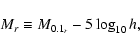 |
(1) |
where M0.1r is the absolute magnitude K-corrected to z=0.1 (kcorrect v3.4) as described in Blanton et al. (2003a).
A volume limited sample of galaxies down to Mr = -18 contains galaxies out to redshift z=0.048, with a median galaxy redshift of z=0.038. The redshift limit is a trade-off with the magnitude limit. I create a ``bright'' sample and a ``faint'' sample, defined such that bright galaxies have r-band magnitudes between -21 and -20 and faint galaxies have magnitudes between -19 and -18. The bright galaxy sample contains galaxies that are near L*, while the faint galaxy sample contains galaxies that have luminosities similar to bright satellites such as the Magellanic Clouds. By excluding objects between Mr= -19 and Mr= -20, the samples are fairly analogous to the samples used in previous works that constrained the spatial distribution of satellite galaxies (e.g., Chen et al. 2006). The corresponding number density of objects for these samples is calculated from the data and shown in Table 1, along with the total number of objects in each sample.
In addition to the faint and bright samples, a luminosity-threshold sample of Mr < -21 and a luminosity-threshold sample of Mr < -19 are created from the same volume-limited sample. These samples are necessary in order to constrain the masses of the halos in which bright and faint galaxies are found, as further described in Sect. 4.
Table 1: Number densities of volume-limited samples of SDSS galaxies.
3 Estimating the correlation function
The correlation function measures the excess probability of finding a pair of objects at some separation, comparing counts of pairs of objects in catalogs of real objects (DD) and in catalogs of objects with randomized positions (RR) and pairs where one object is in the real catalog and its counterpart in the random catalog (DR or RD)![]() . The total number of pairs is normalized by the total number of objects in a sample, such that
. The total number of pairs is normalized by the total number of objects in a sample, such that
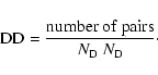 |
(2) |
Using the Landy & Szalay (1993) estimator, the cross-correlation as a function of projected separation,
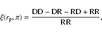 |
(3) |
while the autocorrelation is
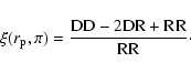 |
(4) |
The parallel and perpendicular components of the pair separations are distinguished in the data by
 |
(5) |
and
 |
(6) |
where
From the correlation function, the projected correlation function is
 |
(7) |
where
Statistical errors in the correlation are estimated via jackknife sampling (see, e.g., Lupton 1993). In the SDSS data, the survey area is divided into 205 equal area samples using the hierarchical pixel scheme SDSSPix, which represents well the rectangular geometry of the SDSS stripes![]() . The covariance matrices are estimated by the covariance between jackknife samples - samples where one of the 205 equal area subsamples is omitted. In order to appropriately estimate the covariance matrix, the number of jackknife samples must be significantly greater than the number of bins in which the correlation function is estimated (Hartlap et al. 2007). Typically, each jackknife sample is constructed to be larger than the largest separation measured in the corresponding correlation function, and the number of jackknife samples is at least equal to the square of the number of bins. With 14 bins, 196 is the minimum number of jackknifes samples. The data sample uses slightly more, 205. The typical jackknife region, then, has a comoving volume of
. The covariance matrices are estimated by the covariance between jackknife samples - samples where one of the 205 equal area subsamples is omitted. In order to appropriately estimate the covariance matrix, the number of jackknife samples must be significantly greater than the number of bins in which the correlation function is estimated (Hartlap et al. 2007). Typically, each jackknife sample is constructed to be larger than the largest separation measured in the corresponding correlation function, and the number of jackknife samples is at least equal to the square of the number of bins. With 14 bins, 196 is the minimum number of jackknifes samples. The data sample uses slightly more, 205. The typical jackknife region, then, has a comoving volume of ![]()
![]() .
The projected cross-correlation and corresponding autocorrelation functions are shown in Fig. 1.
.
The projected cross-correlation and corresponding autocorrelation functions are shown in Fig. 1.
![\begin{figure}
\par\includegraphics[width=7cm,clip]{9184fig1.ps}
\end{figure}](/articles/aa/full_html/2009/06/aa9184-07/img34.gif) |
Figure 1: The measured projected correlation functions in the SDSS data, where the cross-correlation of bright and faint galaxies is indicated by filled circles, the bright autocorrelation by open circles, and the faint autocorrelation by filled triangles. Bright galaxies have r-band magnitudes between -21 and -20, while faint galaxies have r-band magnitudes between -19 and -18. |
| Open with DEXTER | |
In the SDSS spectroscopic survey, no single pointing of the telescope can measure the spectra of objects that are separated by less than
![]() ,
the fiber collision distance. At the median redshift of the sample,
,
the fiber collision distance. At the median redshift of the sample,
![]() is 30 h-1 kpc, well above the minimum separation of 10 h-1 kpc in the data. To achieve the minimum separation, I employ a catalog corrected for collisions. For pairs of objects separated by less than the fiber collision distance in the target selection catalog, the unobserved target is assigned the redshift of the observed object in the pair. This could bias the sample by overestimating pairs, but significant error is unlikely given that pairs at those separations are extremely correlated (as in Fig. 1).
is 30 h-1 kpc, well above the minimum separation of 10 h-1 kpc in the data. To achieve the minimum separation, I employ a catalog corrected for collisions. For pairs of objects separated by less than the fiber collision distance in the target selection catalog, the unobserved target is assigned the redshift of the observed object in the pair. This could bias the sample by overestimating pairs, but significant error is unlikely given that pairs at those separations are extremely correlated (as in Fig. 1).
Previous studies have described systematic errors with angular dependence (Adelman-McCarthy et al. 2008; Mandelbaum et al. 2006a; Masjedi et al. 2006). Issues with sky subtraction may lead to underestimation of pairs by ![]()
![]() with angular separations between
with angular separations between
![]() and an overestimation of pairs at angular separations less than
and an overestimation of pairs at angular separations less than
![]() .
This effect is most acute for pairs of objects that consist of an apparently bright object and an apparently faint object (Mandelbaum 2006, private communication).
.
This effect is most acute for pairs of objects that consist of an apparently bright object and an apparently faint object (Mandelbaum 2006, private communication).
In the cross-correlated sample, the estimated systematic error of 5% for pairs with angular separations between
![]() and
and
![]() is smaller than the statistical errors in the correlation function,
is smaller than the statistical errors in the correlation function, ![]()
![]() ,
indicating that such errors do not affect the results. For the unconstrained overestimate of pairs with angular separations less than
,
indicating that such errors do not affect the results. For the unconstrained overestimate of pairs with angular separations less than
![]() ,
only the first bin of the estimated cross-correlation (containing objects with projected physical separation of less than 16 h-1 kpc) is affected. In this bin, 23% of the pairs could be possibly affected, while the fractional statistical error in the correlation function is 15%. Given that only one of the data points is affected, it seems unlikely that the parameter estimates are biased by this systematic. However, I test the possible effects of this error in Sects. 5.5 and 6.3.
,
only the first bin of the estimated cross-correlation (containing objects with projected physical separation of less than 16 h-1 kpc) is affected. In this bin, 23% of the pairs could be possibly affected, while the fractional statistical error in the correlation function is 15%. Given that only one of the data points is affected, it seems unlikely that the parameter estimates are biased by this systematic. However, I test the possible effects of this error in Sects. 5.5 and 6.3.
4 Halo model of correlation functions
The correlation function can be modeled using the halo model - assuming that all galaxies and dark matter particles live in dark matter halos. First, the correlation function is decomposed into two parts: a one-halo term and a two-halo term,
| (8) |
where the terms correspond to contributions from galaxy pairs found in the same dark matter halo and galaxy pairs found in different halos. At small separations, r, the one-halo term dominates the correlation function, while at large separations, the two-halo term dominates.
All galaxies are identified as either a central galaxy, found at the center of a dark matter halo, or a satellite galaxy, found elsewhere in the halo. Following Tinker et al. (2005, see their Appendices A and B), the one-halo term is decomposed into two additional terms: (1) a central-satellite term where one galaxy of a pair is the central
galaxy and the other is a satellite of the central galaxy and (2) a
satellite-satellite term where both galaxies in a pair are satellite
galaxies in a halo. As in Berlind & Weinberg (2002, Eq. (11)), the one-halo term can be written,
 |
(9) |
where
To separate the central-satellite term from the satellite-satellite term, for the cross-correlation function,
| (10) |
and for the autocorrelation,
| (11) |
where centrals are denoted by ``cen'', satellites are denoted by ``sat'' and bright and faint objects are labeled ``b'' and ``f.''
The two-halo term is more easily calculated in Fourier space, where the power spectrum P(k) is the Fourier transform of the correlation function ![]() :
:
| |
= | ![$\displaystyle P_{\rm m}(k) \left[\frac{1}{\bar{n}_1} \int {\rm d}M_1 \frac{{\rm d}n}{{\rm d}M_1} \langle N \rangle_{M_1} b_h(M_1,r) y_g(k,M_1)\right]$](/articles/aa/full_html/2009/06/aa9184-07/img59.gif) |
|
![$\displaystyle \times \left[\frac{1}{\bar{n}_2} \int {\rm d}M_2 \frac{{\rm d}n}{{\rm d}M_2} \langle N \rangle_{M_2} b_h(M_2,r) y_g(k,M_2)\right],$](/articles/aa/full_html/2009/06/aa9184-07/img60.gif) |
(12) |
where yg(k,M) is the Fourier transform of the halo density profile and
![\begin{displaymath}b^2(M,r) = b^2(M) \frac{\left[1 + 1.17 \xi_{\rm m}(r)\right]^{1.49}}{\left[1 + 0.69 \xi_{\rm m}(r)\right]^{2.09}},
\end{displaymath}](/articles/aa/full_html/2009/06/aa9184-07/img64.gif) |
(13) |
where the scale-independent bias is provided by Tinker et al. (2005, see their Appendix A). They calibrate the analytic model of Sheth & Tormen (1999) with numerical simulations. In addition, the assumption that the separation between halos is much greater than the scale of the halos leads to an overestimate in power at intermediate separations where the one-halo and two-halo terms are comparable - counting pairs in overlapping halos that would rightly be counted as single halos. I use the spherical exclusion approximation from Tinker et al. (2005). They only specify the two-halo term for the autocorrelation. For the cross-correlation, the geometric mean of the the two autocorrelated samples is used as an approximation, which performed well in tests on populated simulations.
While the terms in the calculation for the halo mass function, halo bias, and halo density profile are fixed, the number of galaxies and their spatial distribution in halos is parameterized and fit to the data. I use the HOD prescription for characterizing the galaxy bias, which has been shown in simulations and semi-analytic models to be reasonable (Berlind et al. 2003; Zheng et al. 2005). For luminosity-threshold samples (samples that include all objects brighter than a threshold luminosity) the average number of central galaxies per halo is a step function at a minimum mass,
![]() for
for
![]() and
and
![]() ,
otherwise. For luminosity-binned samples (including all objects within a minimum and maximum luminosity),
,
otherwise. For luminosity-binned samples (including all objects within a minimum and maximum luminosity),
![]() is a step function, with both a minimum mass and a maximum mass:
is a step function, with both a minimum mass and a maximum mass:
![]() for
for
![]()
![]() .
.
For the average number of satellite galaxies, a simple functional form with three parameters is used (Tinker et al. 2005):
 |
(14) |
Using luminosity-threshold samples, simulations show that
For each galaxy sample, there are three free HOD parameters - M1, ![]() ,
and
,
and
![]() - and two fixed HOD parameters -
- and two fixed HOD parameters -
![]() and
and
![]() .
.
![]() is set by the observed number density of objects in the faint or bright sample such that
is set by the observed number density of objects in the faint or bright sample such that
| |
= |  |
|
| = | 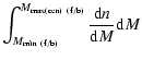 |
||
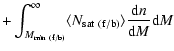 |
(15) |
where
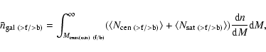 |
(16) |
where
In addition to the HOD parameters described above, parameters to describe the spatial distribution of objects are required. As mentioned previously, the spatial distribution of galaxies is parameterized by f, a scaling factor relating the concentration of a DM halo to the concentration for the distribution of galaxies in that halo, such that
![]() .
The three clustering measures - the faint autocorrelation, the bright autocorrelation, and the cross-correlation - require a total of two such parameters. The first, f, parameterizes the spatial distribution of the autocorrelated samples - i.e., the distribution of any-sized satellite in any mass halo. This comprises a large catalog of objects and smears out environmental differences, e.g., assuming that
.
The three clustering measures - the faint autocorrelation, the bright autocorrelation, and the cross-correlation - require a total of two such parameters. The first, f, parameterizes the spatial distribution of the autocorrelated samples - i.e., the distribution of any-sized satellite in any mass halo. This comprises a large catalog of objects and smears out environmental differences, e.g., assuming that
![]() .
The second,
.
The second,
![]() parameterizes only the distribution of faint satellite galaxies in halos with bright central galaxies, as defined in the samples. This comprises a small number of objects and ensures that the parameter in question measures only the spatial distribution of satellite galaxies in galactic halos with
parameterizes only the distribution of faint satellite galaxies in halos with bright central galaxies, as defined in the samples. This comprises a small number of objects and ensures that the parameter in question measures only the spatial distribution of satellite galaxies in galactic halos with ![]() L* galaxies. The narrowness of the category for
L* galaxies. The narrowness of the category for
![]() ,
however, means that the parameter is constrained by fewer data points than f and depends only on the one-halo central-satellite term of the cross-correlation function, a term which is only dominant in the correlation function for separations less than
,
however, means that the parameter is constrained by fewer data points than f and depends only on the one-halo central-satellite term of the cross-correlation function, a term which is only dominant in the correlation function for separations less than ![]() 0.1 h-1 Mpc.
0.1 h-1 Mpc.
I simultaneously fit the cross-correlation function of the bright and faint samples, the autocorrelation function of the bright sample, and autocorrelation of the faint sample, which requires eight free HOD parameters: 3 parameters - M1, ![]() ,
and
,
and
![]() - for the faint and bright sample each and 2 parameters, f and
- for the faint and bright sample each and 2 parameters, f and
![]() ,
to describe the spatial distribution of objects in halos.
,
to describe the spatial distribution of objects in halos.
5 Parameter fitting with Monte Carlo Markov Chains
5.1 MCMC
To estimate the best-fit parameters and constrain the errors in their values, I use a Monte Carlo Markov Chain (MCMC) method. The algorithm explores the probability distributions of a large number of parameters such that the distribution of points in parameter space visited by an infinitely long MCMC chain follows the underlying probability density exactly. MCMC both measures the best-fit parameters and constrains the errors in the parameter estimation and a sufficiently long chain will not be hampered by local minima in the parameter space.
A MCMC chain is created by choosing points in the parameter space based on a trial distribution around the previous point in the chain, stepping along
the eigenvectors of the covariance matrix of the parameters. Trial steps that result in a smaller ![]() are
accepted while steps that do not are accepted with some probability,
are
accepted while steps that do not are accepted with some probability,
![]() .
For a finite chain, when the distribution of steps reflects the underlying distribution with sufficient accuracy, the chain is said to have converged. In addition, if a chain is started far outside the region of high probability, an initial section will be unrepresentative and must be discarded; this initial section is referred to as ``burn in.'' This truncation is unnecessary or can be minimized if the chain is started from a point already known to lie in the region of high probability. For my chains, I start the MCMC at the point in parameter space that has been identified as the likelihood maximum using a simple downhill simplex
.
For a finite chain, when the distribution of steps reflects the underlying distribution with sufficient accuracy, the chain is said to have converged. In addition, if a chain is started far outside the region of high probability, an initial section will be unrepresentative and must be discarded; this initial section is referred to as ``burn in.'' This truncation is unnecessary or can be minimized if the chain is started from a point already known to lie in the region of high probability. For my chains, I start the MCMC at the point in parameter space that has been identified as the likelihood maximum using a simple downhill simplex ![]() minimization algorithm for the data. For good measure, the trial steps are examined for large-scale modes indicative of burn-in and convergence is tested by calculation of the power spectrum of the chain as is described by Dunkley et al. (2005).
minimization algorithm for the data. For good measure, the trial steps are examined for large-scale modes indicative of burn-in and convergence is tested by calculation of the power spectrum of the chain as is described by Dunkley et al. (2005).
5.2 Testing parameter estimates with mock galaxy catalogs
To test the constraining power of my sample using this method, I create test catalogs, populating halos from a numerical simulation with reasonably-chosen values for the HOD parameters![]() . Analyzing this mock data and comparing the derived HOD parameters to the input will show how well the analysis can work and how good the data needs to be for the analysis to provide robust constraints. The HOD parameters are listed in Table 2. For the spatial distribution, both f=1 and
. Analyzing this mock data and comparing the derived HOD parameters to the input will show how well the analysis can work and how good the data needs to be for the analysis to provide robust constraints. The HOD parameters are listed in Table 2. For the spatial distribution, both f=1 and
![]() .
MCMC is used to find the best-fit values of the eight free parameters and characterize the error distributions.
.
MCMC is used to find the best-fit values of the eight free parameters and characterize the error distributions.
Table 2: HOD parameters for mock data sets.
The simulation used here was performed using the Hashed Oct-Tree code of Warren & Salmon (1993), and is similar to those presented in Seljak & Warren (2004) and Warren et al. (2006). The simulation box is
400 h-1 Mpc on a side with 12803 particles and a particle mass of
![]() .
Halos are identified by the friends-of-friend technique (Davis et al. 1985) with a linking length of 0.2 times the mean interparticle separation. For galaxies in my faint sample, the corresponding halo in the simulation has roughly
.
Halos are identified by the friends-of-friend technique (Davis et al. 1985) with a linking length of 0.2 times the mean interparticle separation. For galaxies in my faint sample, the corresponding halo in the simulation has roughly ![]() 100 particles. The simulation uses a cosmology of
100 particles. The simulation uses a cosmology of
![]() ,
,
![]() ,
,
![]() ,
h=0.7, and
,
h=0.7, and
![]() ;
I use the output at the redshift of z=0.0.
;
I use the output at the redshift of z=0.0.
I create two volumes of mock data. In the first, I use the full simulation box to look for biases in finding the best-fit values for the HOD parameters and to describe the degeneracies between parameters. In the second, I use a volume of data similar to the volume of available data to show how well the analysis will work on the real data and how robust the the constraints will be. I also use this volume of data to test systematics in the SDSS data and the ability of the method to recover different values for f and
![]() .
.
5.3 Tests using idealized mock data set
The full simulation box of 400 h-1 Mpc on a side is 42 times the volume of the volume-limited SDSS data set. For this box, I calculate the bright and faint galaxy autocorrelations, the cross-correlation, and all associated covariance matrices using 400 jackknife samples. Using the full simulation box, the diagonal errors on the faint autocorrelation and the cross-correlation functions are significantly less than 5%. The errors on the dark matter power spectrum (Smith et al. 2003), however, are likely larger than 5%. Analyzing the full simulation box, then, will only constrain the errors on the dark matter power spectrum and say nothing about the biases in and degeneracies between HOD parameters. In order to evade this problem, I replace the measured faint autocorrelation and the cross-correlation with the exact values for the chosen HOD.
Table 3: Unmarginalized, best-fit parameters for mock data sets.
In Table 3, the derived best-fit parameters are listed along with their unmarginalized 68% errors, constraining f and
![]() to within
to within ![]() .
The table shows that the true values of all the parameters fall within the 68% confidence intervals. Deviations from true parameter values may be attributed in part to degeneracies between parameters, to sample variance, or to approximations in the calculation of the correlation function, such as use of spherical halo exclusion in place of elliptical exclusion.
.
The table shows that the true values of all the parameters fall within the 68% confidence intervals. Deviations from true parameter values may be attributed in part to degeneracies between parameters, to sample variance, or to approximations in the calculation of the correlation function, such as use of spherical halo exclusion in place of elliptical exclusion.
Degeneracies between pairs of parameters are investigated in Fig. 2. In each panel, the 68% and 90% confidence intervals are shown, marginalizing over all other parameters. f and
![]() are more degenerate with the faint HOD parameters than the bright parameters. The faint sample has many more objects than the bright sample, so its constraining ability is greater. In addition,
are more degenerate with the faint HOD parameters than the bright parameters. The faint sample has many more objects than the bright sample, so its constraining ability is greater. In addition,
![]() is only constrained by the one-halo, central-satellite term of the cross-correlation, which depends only on the faint HOD parameters. However, the degeneracies between HOD parameters - M1,
is only constrained by the one-halo, central-satellite term of the cross-correlation, which depends only on the faint HOD parameters. However, the degeneracies between HOD parameters - M1, ![]() ,
,
![]() - in a single sample are much larger. Finally, the degeneracy between f and
- in a single sample are much larger. Finally, the degeneracy between f and
![]() is pronounced and behaves such that larger values of f are accompanied by larger values of
is pronounced and behaves such that larger values of f are accompanied by larger values of
![]() and vice versa.
and vice versa.
![\begin{figure}
\par\includegraphics[width=8cm,clip]{9184fig2a.ps}\hspace*{4mm}
\includegraphics[width=6.8cm,clip]{9184fig2b.ps}
\end{figure}](/articles/aa/full_html/2009/06/aa9184-07/img114.gif) |
Figure 2:
The 68 and 90% marginalized confidence intervals are shown for pairs of parameters in the idealized data set. All masses are shown in log(
|
| Open with DEXTER | |
The behavior of these degeneracies can be seen from the form of the HOD itself. Compared to an arbitrary satellite function,
![]() ,
increasing the parameter M1 reduces the overall number of satellites. This, however, can be compensated at masses larger than M1 by increasing the slope,
,
increasing the parameter M1 reduces the overall number of satellites. This, however, can be compensated at masses larger than M1 by increasing the slope, ![]() .
At smaller masses, increasing M1 and
.
At smaller masses, increasing M1 and ![]() reduces the fraction of central-satellite pairs. Decreasing the roll-off parameter,
reduces the fraction of central-satellite pairs. Decreasing the roll-off parameter,
![]() ,
marginally increases the fraction of central-satellite pairs. Thus, larger M1 indicates larger
,
marginally increases the fraction of central-satellite pairs. Thus, larger M1 indicates larger ![]() and smaller
and smaller
![]() .
In relation to the parameter f, increasing
.
In relation to the parameter f, increasing ![]() tilts the correlation function to pairs in halos with larger masses and smaller concentrations; increasing f and
tilts the correlation function to pairs in halos with larger masses and smaller concentrations; increasing f and
![]() counteracts this by boosting the concentrations.
counteracts this by boosting the concentrations.
5.4 Tests using SDSS-sized mock data set
A subsample of the simulation box that is 115 h-1 Mpc on a side is equal in volume to the SDSS data sample. Using 196 jackknife samples (similar to the 205 samples used in the data) and estimating all correlations and covariances from the simulation, the size of the error bars are larger than in the case of the idealized box.
The results of the parameter estimation are shown in Table 3 and are particularly striking in the case of the roll-off parameter,
![]() ,
where the parameter space of likely values extends to
,
where the parameter space of likely values extends to
![]() .
Once
.
Once
![]() drops below the minimum mass for central galaxies, it no longer has any effect on the correlation function, resulting in extremely large errors on the parameter estimation. At the volume of the SDSS data set, f=1 can be distinguished from f=2, but values of
drops below the minimum mass for central galaxies, it no longer has any effect on the correlation function, resulting in extremely large errors on the parameter estimation. At the volume of the SDSS data set, f=1 can be distinguished from f=2, but values of
![]() are consistent.
are consistent.
The resulting errors in the parameter estimation are not directly applicable to the SDSS data. In addition to the issue of sample variance, the populated simulations are an idealized dataset where the halos are exactly populated according to a HOD, there is no variance in the concentration of halos, and the cosmology of the populated simulation is the same as that used in the model. The presented analysis, however, demonstrates approximately the degree to which the HOD and the radial distribution of satellites can be constrained with the current volume-limited SDSS sample.
5.5 Tests including systematics and varying f and f cross
Using the SDSS-sized mock data set, I include the effects of the systematics in the SDSS data: 1) issues with the sky subtraction (see Sect. 3) and 2) incompleteness in the spectroscopic catalog (see Sect. 2).
As discussed previously, the sky subtraction problem is angle dependent, over-predicting pairs at separations less than
![]() and under-predicting by
and under-predicting by ![]()
![]() pairs at separations between
pairs at separations between
![]() .
At the median redshift of the data,
.
At the median redshift of the data,
![]() is 16 h-1 kpc. The overestimate in pairs at small angular separations is unconstrained, but in the data
is 16 h-1 kpc. The overestimate in pairs at small angular separations is unconstrained, but in the data ![]()
![]() of the objects in the first bin of the correlation function (from 10 to 16 h-1 kpc) are found at separations less than
of the objects in the first bin of the correlation function (from 10 to 16 h-1 kpc) are found at separations less than
![]() .
I assume that all of the 25% are spurious pairs and add that fraction of pairs into the mock data at separations less than 16 h-1 kpc.
.
I assume that all of the 25% are spurious pairs and add that fraction of pairs into the mock data at separations less than 16 h-1 kpc.
![]() is
22-50 h-1 kpc at the median redshift of the data. In the mock data, I remove 5% of the pairs with separations between 22 and 50 h-1 kpc.
is
22-50 h-1 kpc at the median redshift of the data. In the mock data, I remove 5% of the pairs with separations between 22 and 50 h-1 kpc.
In addition to including these refinements, I test different values of f and
![]() in order to show that a range of values can be reproduced. The catalogs produced are MA1 (f=0.5,
in order to show that a range of values can be reproduced. The catalogs produced are MA1 (f=0.5,
![]() ); MB1 (f=1,
); MB1 (f=1,
![]() ); and MC1 (f=1,
); and MC1 (f=1,
![]() ). I also create a sample MA2 where the global completeness is exactly 90%. This overstates the effect of incompleteness in the data where I use all areas with completeness better than 90%.
). I also create a sample MA2 where the global completeness is exactly 90%. This overstates the effect of incompleteness in the data where I use all areas with completeness better than 90%.
Results are shown in Table 4. While the errors in these cases can be larger than the errors without accounting for systematic effects, there are no biases in the estimated HOD values and a full range of values for f and
![]() are recoverable from the data.
are recoverable from the data.
Table 4:
Unmarginalized, best-fit f and
![]() for mock data sets.
for mock data sets.
6 Results
The analysis applied to the test samples can be repeated for the SDSS samples. First, the values of
![]() for the bright and faint sample must be estimated. With those values, the fiducial results for the HOD parameters can be found. Then, the robustness of the best-fit values of f and
for the bright and faint sample must be estimated. With those values, the fiducial results for the HOD parameters can be found. Then, the robustness of the best-fit values of f and
![]() is tested. Finally, the results are compared to weak lensing results.
is tested. Finally, the results are compared to weak lensing results.
6.1 Estimating Mmax(cen)
The maximum halo mass,
![]() ,
for the bright and faint samples must be measured from additional SDSS samples as described in Sect. 4. A luminosity-threshold sample of
Mr < -21 is used to calculate
,
for the bright and faint samples must be measured from additional SDSS samples as described in Sect. 4. A luminosity-threshold sample of
Mr < -21 is used to calculate
![]() for the bright sample and a luminosity-threshold sample of
Mr < -19 is used for the faint sample. For the
Mr < -19 sample, I fit 4 parameters, M1,
for the bright sample and a luminosity-threshold sample of
Mr < -19 is used for the faint sample. For the
Mr < -19 sample, I fit 4 parameters, M1, ![]() ,
,
![]() ,
and f. For the
Mr < -21 sample, the number of objects with projected separations less than
,
and f. For the
Mr < -21 sample, the number of objects with projected separations less than
![]() Mpc is small, so constraints on f are extremely difficult to obtain, and I set f=1 and fit only 3 parameters.
Mpc is small, so constraints on f are extremely difficult to obtain, and I set f=1 and fit only 3 parameters.
Table 5: HOD parameters for SDSS luminosity-threshold samples.
The best-fit values and the smallest and largest values for
![]() for the unmarginalized parameter space that contains 68% of the values estimated by MCMC are listed in Table 5. Even using luminosity-threshold samples, however, the range of values for the bright and faint
for the unmarginalized parameter space that contains 68% of the values estimated by MCMC are listed in Table 5. Even using luminosity-threshold samples, however, the range of values for the bright and faint
![]() is rather large, with some
is rather large, with some ![]() 20-30% variation in the faint sample and less than
20-30% variation in the faint sample and less than ![]()
![]() variation in the bright sample. Previously published results using different volumes of SDSS data find similar, but not identical results. For example, Zehavi et al. (2005) - which fixes f=1 - find for their Mr < -21 sample that
variation in the bright sample. Previously published results using different volumes of SDSS data find similar, but not identical results. For example, Zehavi et al. (2005) - which fixes f=1 - find for their Mr < -21 sample that
![]() ,
,
![]() ,
and
,
and
![]() .
For their Mr < -19 sample, they find
.
For their Mr < -19 sample, they find
![]() ,
,
![]() ,
and
,
and
![]() .
.
6.2 Fiducial results for f and f cross
Table 6:
Unmarginalized, best-fit parameters for SDSS data using best-fit
![]() .
.
Using the best-fit values for
![]() ,
the best-fit HOD parameters for the luminosity-binned samples are found and shown in Fig. 3 along with the best-fit cross-correlation. The unmarginalized best-fit parameters are listed in Table 6. The marginalized likelihoods for the parameters are shown in Fig. 4.
,
the best-fit HOD parameters for the luminosity-binned samples are found and shown in Fig. 3 along with the best-fit cross-correlation. The unmarginalized best-fit parameters are listed in Table 6. The marginalized likelihoods for the parameters are shown in Fig. 4.
![\begin{figure}
\par\includegraphics[width=7.6cm,clip]{9184fig3.ps}
\end{figure}](/articles/aa/full_html/2009/06/aa9184-07/img162.gif) |
Figure 3: Top: the estimated cross-correlation ( circles) compared to the halo model cross-correlation using the best-fit HOD parameters ( solid line). Bottom: the shape of the HOD for the bright sample ( dotted) and the faint sample ( solid). |
| Open with DEXTER | |
![\begin{figure}
\par\includegraphics[width=7.6cm,clip]{9184fig4.ps}
\end{figure}](/articles/aa/full_html/2009/06/aa9184-07/img163.gif) |
Figure 4:
The normalized, marginalized likelihoods for all parameters (M1, |
| Open with DEXTER | |
As expected from the tests of the mock data sets, the value of
![]() is not well-constrained by the data, although the best-fit values suggest that the galaxy distribution is consistent with the expected DM distribution,
is not well-constrained by the data, although the best-fit values suggest that the galaxy distribution is consistent with the expected DM distribution,
![]() .
There is a wide range of values from
.
There is a wide range of values from ![]() .5 to
.5 to ![]() 2 within the unmarginalized 68% error ellipse. Extremely small values, however, are not supported (
2 within the unmarginalized 68% error ellipse. Extremely small values, however, are not supported (
![]() ). f, as expected, is better constrained, with values from
). f, as expected, is better constrained, with values from ![]() .2 and
.2 and ![]() 1 within the unmarginalized 68% error ellipse. f<1 is very probable. This may suggest that the distribution of galaxies is shallower than the dark matter distribution, which would still be consistent with previous work at galaxy and cluster scales (e.g., Nagai & Kravtsov 2005; Chen et al. 2006). Finally, recalling the degeneracy between f and
1 within the unmarginalized 68% error ellipse. f<1 is very probable. This may suggest that the distribution of galaxies is shallower than the dark matter distribution, which would still be consistent with previous work at galaxy and cluster scales (e.g., Nagai & Kravtsov 2005; Chen et al. 2006). Finally, recalling the degeneracy between f and
![]() ,
if one were to guess that the best-fit estimate of f was biased to smaller values, one would also have to assume that the most likely value of
,
if one were to guess that the best-fit estimate of f was biased to smaller values, one would also have to assume that the most likely value of
![]() is also too small.
is also too small.
6.3 Tests of the robustness of the fiducial results
In addition to the fiducial data set, I test a shortened data set, omitting the first bin in the correlation functions (physical separations smaller than 16 h-1 kpc), with unmarginalized results also shown in Table 6. As discussed in Sect. 3, this bin is most affected by sky subtraction issues in the photometry. Omitting it does not appreciably change any of the results, aside from inflating the error bar on
![]() ,
the parameter most sensitive to small projected separations.
,
the parameter most sensitive to small projected separations.
Because
![]() is estimated from different luminosity samples than the faint and bright samples, I test the effects of the variances in
is estimated from different luminosity samples than the faint and bright samples, I test the effects of the variances in
![]() estimates. I run the MCMC for four samples, changing in turn the bright and faint
estimates. I run the MCMC for four samples, changing in turn the bright and faint
![]() to the lower and the upper value in the 68% unmarginalized confidence intervals and leaving the other
to the lower and the upper value in the 68% unmarginalized confidence intervals and leaving the other
![]() fixed to the fiducial value. The test samples are described and results are presented in Table 7. Here, the parameter estimates look very similar to the fiducial values, except in the case where a lower estimate of
fixed to the fiducial value. The test samples are described and results are presented in Table 7. Here, the parameter estimates look very similar to the fiducial values, except in the case where a lower estimate of
![]() in the bright sample was used. In all cases, however, the errors overlap and all show consistent results of
in the bright sample was used. In all cases, however, the errors overlap and all show consistent results of
![]() .
.
Table 7:
Unmarginalized, best-fit parameters for SDSS data varying
![]() .
.
In Fig. 4, the parameter
![]() has an oddly shaped and broad likelihood distribution (discussed briefly in the previous section). The marginalized likelihoods for
has an oddly shaped and broad likelihood distribution (discussed briefly in the previous section). The marginalized likelihoods for
![]() in the SDSS data suggest rather small values. As noted previously, when
in the SDSS data suggest rather small values. As noted previously, when
![]() ,
,
![]() contributes nothing to the HOD. One may be tempted to suggest that the small
contributes nothing to the HOD. One may be tempted to suggest that the small
![]() values are due to poor constraints of the data. However, small values may be well-motivated, at least for the bright sample. As the bright
values are due to poor constraints of the data. However, small values may be well-motivated, at least for the bright sample. As the bright
![]() increases, the amplitude at small scales in the autocorrelation, where the one-halo central-satellite term dominates, decreases. The amplitude in the cross-correlation, however, is unaffected, since the central-satellite term in the cross-correlation samples the part of the faint sample satellite distribution that is unaffected by
increases, the amplitude at small scales in the autocorrelation, where the one-halo central-satellite term dominates, decreases. The amplitude in the cross-correlation, however, is unaffected, since the central-satellite term in the cross-correlation samples the part of the faint sample satellite distribution that is unaffected by
![]() .
Thus, large values of
.
Thus, large values of
![]() for the bright sample would cause the bright autocorrelation and the cross-correlation to intersect, which is not supported by the data (see Fig. 1).
for the bright sample would cause the bright autocorrelation and the cross-correlation to intersect, which is not supported by the data (see Fig. 1).
6.4 Comparison to weak lensing results
If satellites are found around galaxies with the same distribution as the dark matter profile, the cross-correlation of bright and faint galaxies may be related to the galaxy-mass cross-correlation. The projected galaxy-mass cross-correlation is proportional to the weak lensing measurement of the surface density contrast,
![]() .
Given the larger errors in the weak lensing measurements at the scales at which the satellite distribution and the dark matter distribution can be compared, a comparison of simple power-law fits may be sufficient, assuming a pure power-law density profile for
.
Given the larger errors in the weak lensing measurements at the scales at which the satellite distribution and the dark matter distribution can be compared, a comparison of simple power-law fits may be sufficient, assuming a pure power-law density profile for
![]() at and below those scales.
at and below those scales.
In comparison to the weak lensing measurement, the cross-correlation of bright and faint galaxies has a somewhat steeper overall power-law slope than the weak-lensing measuring. For example, Sheldon et al. (2004) find a power-law slope of
![]() for projected radii between 0.025 and 10 h-1 Mpc and their lens sample is peaked near an r-band magnitude of -21. In addition, comparisons to the measurements from Mandelbaum et al. (2006b) for a lens sample with r-band magnitudes between -21 and -20 show similar power-law slopes,
for projected radii between 0.025 and 10 h-1 Mpc and their lens sample is peaked near an r-band magnitude of -21. In addition, comparisons to the measurements from Mandelbaum et al. (2006b) for a lens sample with r-band magnitudes between -21 and -20 show similar power-law slopes,
![]() for projected radii between 0.02 and 2 h-1 Mpc. Both measurements are shallower than the power-law slope of the cross-correlation of bright and faint galaxies, which show
for projected radii between 0.02 and 2 h-1 Mpc. Both measurements are shallower than the power-law slope of the cross-correlation of bright and faint galaxies, which show
![]() at projected radii between 0.01 and 16 h-1 Mpc
at projected radii between 0.01 and 16 h-1 Mpc![]() .
.
The cross-correlation function, however, is more sensitive to the distribution of satellites around central galaxies at smaller separations. The best-fit power-law slope for the projected cross-correlation remains fairly consistent, with
![]() for projected radii between 0.01 and 0.25 h-1 Mpc and
for projected radii between 0.01 and 0.25 h-1 Mpc and
![]() for projected radii between 0.01 and 0.1 h-1 Mpc. Mandelbaum et al. (2006b) shows larger error bars at small radii, with rough consistency with my results,
for projected radii between 0.01 and 0.1 h-1 Mpc. Mandelbaum et al. (2006b) shows larger error bars at small radii, with rough consistency with my results,
![]() for projected radii between 0.02 and 0.2 h-1 Mpc and
for projected radii between 0.02 and 0.2 h-1 Mpc and
![]() for projected radii between 0.02 and 0.1 h-1 Mpc. The best-fit power-laws for the cross-correlation of bright and faint galaxies and the galaxy-mass cross-correlation around bright galaxies are statistically consistent at the most significant separations. This is consistent with a result of
for projected radii between 0.02 and 0.1 h-1 Mpc. The best-fit power-laws for the cross-correlation of bright and faint galaxies and the galaxy-mass cross-correlation around bright galaxies are statistically consistent at the most significant separations. This is consistent with a result of
![]() - the satellite distribution follows the DM halo distribution.
- the satellite distribution follows the DM halo distribution.
7 Conclusions
The spatial distribution of satellite galaxies around ![]() L* galaxies can illuminate the relationship between satellite galaxies and dark matter subhalos and aid in developing and testing galaxy formation models. The projected cross-correlation of bright galaxies with faint galaxies offers a promising avenue to putting constraints on the radial distribution of satellite galaxies.
L* galaxies can illuminate the relationship between satellite galaxies and dark matter subhalos and aid in developing and testing galaxy formation models. The projected cross-correlation of bright galaxies with faint galaxies offers a promising avenue to putting constraints on the radial distribution of satellite galaxies.
Results from SDSS data of 5104
![]() on the sky suggest that the spatial distribution of galaxies, parameterized by f and
on the sky suggest that the spatial distribution of galaxies, parameterized by f and
![]() ,
is generally consistent with the dark matter distribution for halos in a flat
,
is generally consistent with the dark matter distribution for halos in a flat ![]() CDM cosmology with
CDM cosmology with
![]() ,
,
![]() ,
,
![]() ,
and h=0.7.
,
and h=0.7.
![]() parameterizes the distribution of ``faint'' satellites galaxies around ``bright'' central galaxies. There are no strong constraints on the value of
parameterizes the distribution of ``faint'' satellites galaxies around ``bright'' central galaxies. There are no strong constraints on the value of
![]() ,
however, with a wide range of values from
,
however, with a wide range of values from ![]() .5 to
.5 to ![]() 2 in the unmarginalized 68% error ellipse, where
2 in the unmarginalized 68% error ellipse, where
![]() would indicate a distribution equivalent to the DM halo profile. f, on the other hand, parameterizes the distribution of both bright and faint satellite galaxies around central galaxies of all sizes. Constraints on the value of f are significantly better - ruling out f=2 - and are suggestive of somewhat smaller concentrations for galaxy distributions compared to the concentration of dark matter halos (f<1). The spatial distribution of galactic satellites remains poorly constrained and future studies in this field will require a greater volume of data.
would indicate a distribution equivalent to the DM halo profile. f, on the other hand, parameterizes the distribution of both bright and faint satellite galaxies around central galaxies of all sizes. Constraints on the value of f are significantly better - ruling out f=2 - and are suggestive of somewhat smaller concentrations for galaxy distributions compared to the concentration of dark matter halos (f<1). The spatial distribution of galactic satellites remains poorly constrained and future studies in this field will require a greater volume of data.
The results presented here use a flat ![]() CDM cosmology with
CDM cosmology with
![]() which is consistent with the results of the Wilkinson Microwave Anisotropy Probe (WMAP) 1-Year Data (Spergel et al. 2003). Recent results from the WMAP 5-Year Data supports a smaller
which is consistent with the results of the Wilkinson Microwave Anisotropy Probe (WMAP) 1-Year Data (Spergel et al. 2003). Recent results from the WMAP 5-Year Data supports a smaller
![]() (Dunkley et al. 2008). Duffy et al. (2008) claim that halo concentrations using a WMAP5 cosmology are lower than in a WMAP1 cosmology by 16-23%. If halos are less concentrated than the model predicts, the fit can compensate by decreasing f. Since f is defined relative to the profile of the DM halo, this implies that the true f and
(Dunkley et al. 2008). Duffy et al. (2008) claim that halo concentrations using a WMAP5 cosmology are lower than in a WMAP1 cosmology by 16-23%. If halos are less concentrated than the model predicts, the fit can compensate by decreasing f. Since f is defined relative to the profile of the DM halo, this implies that the true f and
![]() are actually larger than the estimated f and
are actually larger than the estimated f and
![]() .
The difference in halo concentration is, however, fairly modest compared to the error estimate in f and
.
The difference in halo concentration is, however, fairly modest compared to the error estimate in f and
![]() .
.
The results of this study have implications for previous works on constraining the satellite spatial distribution, galaxy clustering models, and weak lensing studies of the galaxy-mass cross-correlation. For example, the results are consistent with those of Chen et al. (2006): satellite galaxies are distributed in a way that is consistent with or less concentrated than the dark matter distribution. The results of Chen et al. (2006) apply only to isolated galaxies, while the cross-correlation approach applies to any parent galaxy. This suggests that the environment of parent galaxies is relatively unimportant. My result is also generally consistent with cluster-sized simulations which include cooling and star formation. In such simulations, while the distribution of dark matter subhalos is less concentrated than the dark matter, the stellar components of satellite galaxies more closely follow the dark matter distribution (Macciò et al. 2006; Nagai & Kravtsov 2005). However, the possible discrepancy in values for f and
![]() suggest that the spatial distribution of a class of satellite objects may depend on the size of the host halo: galaxy-sized halos, groups and clusters.
suggest that the spatial distribution of a class of satellite objects may depend on the size of the host halo: galaxy-sized halos, groups and clusters.
Chen (2008) suggest that the projected radial distribution of satellite galaxies depends upon satellite color, such that redder satellites have a significantly steeper density profile than bluer satellites. A cross-correlation analysis with a different selection function for satellites then should show such a color dependence. In order to achieve better constraints on the spatial distribution of satellite galaxies and its environmental and color dependency, larger data sets are required. One possibility for increasing the volume of data is to apply a similar analysis to the photometric redshift catalog, instead of limiting the sample to objects with spectroscopic redshifts. The SDSS photometric redshift catalog goes far deeper than the spectroscopic catalog and without the spectroscopic catalog's fiber collision problem. However, photometric redshifts are less accurate and may complicate the statistical error analysis. Given that future large surveys such as the Dark Energy Survey and the Panoramic Survey Telescope & Rapid Response System (Pan-STARRS) which will produce significantly more photometric redshifts than currently available, it would be interesting to perform a cross-correlation analysis with photometric redshifts.
Acknowledgements
An incredible number of people need to acknowledged for their invaluable contributions. I would like to thank Jeremy Tinker for allowing me to use and modify his halo model code, and Zheng Zheng for his help with additions to the analysis code. I would also like to thank Michael Warren for allowing me to use his simulations, Risa Wechsler and Charlie Conroy for providing me with luminosity assigned galaxy catalogs, and Michael Blanton and Morad Masjedi for useful discussions about the data. In addition, Erin Sheldon and Rachel Mandelbaum were extremely helpful in discussions of the data, its systematics, and weak lensing observations, as was Ryan Scranton in sharing his code to create jackknife samples. Eduardo Rozo, Douglas Rudd, and Sean Andrews each provided useful advice on a variety of topics. Finally, I would like to thank my adviser, Andrey Kravtsov, for his guidance and insight.
This research was carried out at the University of Chicago, Kavli Institute for Cosmological Physics and was supported (in part) by grant NSF PHY-0114422. KICP is an NSF Physics Frontier Center. J.C. was supported by the National Science Foundation (NSF) under grants No. AST-0206216, AST-0239759 and AST-0507666, and by NASA through grant NAG5-13274.
Funding for the Sloan Digital Sky Survey (SDSS) has been provided by the Alfred P. Sloan Foundation, the Participating Institutions, the National Aeronautics and Space Administration, the National Science Foundation, the U.S. Department of Energy, the Japanese Monbukagakusho, and the Max Planck Society. The SDSS Web site is http://www.sdss.org/.
The SDSS is managed by the Astrophysical Research Consortium (ARC) for the Participating Institutions. The Participating Institutions are The University of Chicago, Fermilab, the Institute for Advanced Study, the Japan Participation Group, The Johns Hopkins University, Los Alamos National Laboratory, the Max-Planck-Institute for Astronomy (MPIA), the Max-Planck-Institute for Astrophysics (MPA), New Mexico State University, University of Pittsburgh, Princeton University, the United States Naval Observatory, and the University of Washington.
References
- Abazajian, K., Zheng, Z., Zehavi, I., et al. 2005, ApJ, 625, 613 [NASA ADS] [CrossRef]
- Adelman-McCarthy, J. K., Jennifer, K., Aguëros, M. A., et al. 2006, ApJS, 162, 38 [NASA ADS] [CrossRef] (In the text)
- Adelman-McCarthy, J. K., Jennifer, K., Aguëros, M. A., et al. 2008, ApJS, 175, 297 [NASA ADS] [CrossRef]
- Azzaro, M., Patiri, S. G., Prada, F., & Zentner, A. R. 2007, MNRAS, 376, L43 [NASA ADS]
- Berlind, A. A., & Weinberg, D. H. 2002, ApJ, 575, 587 [NASA ADS] [CrossRef]
- Berlind, A. A., Weinberg, D. H., Benson, A. J., et al. 2003, ApJ, 593, 1 [NASA ADS] [CrossRef]
- Blanton, M. R., Brinkmann, J., Csabai, I., et al. 2003a, AJ, 125, 2348 [NASA ADS] [CrossRef] (In the text)
- Blanton, M. R., Lin, H., Lupton, R. H., et al. 2003b, AJ, 125, 2276 [NASA ADS] [CrossRef]
- Blanton, M. R., Schlegel, D. J., Strauss, M. A., et al. 2005, AJ, 129, 2562 [NASA ADS] [CrossRef] (In the text)
- Brainerd, T. G. 2005, ApJ, 628, L101 [NASA ADS] [CrossRef]
- Bullock, J. S., Kolatt, T. S., Sigad, Y., et al. 2001, MNRAS, 321, 559 [NASA ADS] [CrossRef] (In the text)
- Chen, J. 2008, A&A, 484, 347 [NASA ADS] [CrossRef] [EDP Sciences] (In the text)
- Chen, J., Kravtsov, A. V., Prada, F., et al. 2006, ApJ, 647, 86 [NASA ADS] [CrossRef] (In the text)
- Colín, P., Klypin, A. A., Kravtsov, A. V., & Khokhlov, A. M. 1999, ApJ, 523, 32 [CrossRef]
- Conroy, C., Newman, J. A., Davis, M., et al. 2005, ApJ, 635, 982 [NASA ADS] [CrossRef]
- Conroy, C., Wechsler, R. H., & Kravtsov, A. V. 2006, ApJ, 647, 201 [NASA ADS] [CrossRef] (In the text)
- Davis, M., Efstathiou, G., Frenk, C. S., & White, S. D. M. 1985, ApJ, 292, 371 [NASA ADS] [CrossRef] (In the text)
- De Lucia, G., Kauffmann, G., Springel, V., et al. 2004, MNRAS, 348, 333 [NASA ADS] [CrossRef]
- Diemand, J., Moore, B., & Stadel, J. 2004, MNRAS, 352, 535 [NASA ADS] [CrossRef]
- Diemand, J., Madau, P., & Moore, B. 2005, MNRAS, 364, 367 [NASA ADS]
- Duffy, A. R., Schaye, J., Kay, S. T., & Dalla Vecchia, C. 2008, MNRAS, 390, L64 [NASA ADS] (In the text)
- Dunkley, J., Bucher, M., Ferreira, P. G., Moodley, K., & Skordis, C. 2005, MNRAS, 356, 925 [NASA ADS] [CrossRef] (In the text)
- Dunkley, J., et al. 2008, ApJS, accepted [arXiv:0803.0586] (In the text)
- Faltenbacher, A., & Diemand, J. 2006, MNRAS, 369, 1698 [NASA ADS] [CrossRef]
- Fisher, K. B., Davis, M., Strauss, M. A., Yahil, A., & Huchra, J. 1994, MNRAS, 266, 50 (In the text)
- Fukugita, M., Ichikawa, T., Gunn, J. E., et al. 1996, AJ, 111, 1748 [NASA ADS] [CrossRef]
- Gao, L., White, S. D. M., Jenkins, A., Stoehr, F., & Springel, V. 2004, MNRAS, 355, 819 [NASA ADS] [CrossRef]
- Ghigna, S., Moore, B., Governato, F., et al. 1998, MNRAS, 300, 146 [CrossRef]
- Ghigna, S., Moore, B., Governato, F., et al. 2000, ApJ, 544, 616 [NASA ADS] [CrossRef]
- Gunn, J. E., Carr, M., Rockosi, C., et al. 1998, AJ, 116, 3040 [NASA ADS] [CrossRef]
- Gunn, J. E., Siegmund, W. A., Mannery, E. J., et al. 2006, AJ, 131, 2332 [NASA ADS] [CrossRef]
- Hartlap, J., Simon, P., & Schneider, P. 2007, A&A, 464, 399 [NASA ADS] [CrossRef] [EDP Sciences] (In the text)
- Hogg, D. W., Finkbeiner, D. P., Schlegel, D. J., & Gunn, J. E. 2001, AJ, 122, 2129 [CrossRef]
- Ivezic, Z., Lupton, R. H., Schlegel, D., et al. 2004, Astron. Nachr., 325, 583 [NASA ADS] [CrossRef]
- Jenkins, A., Frenk, C. S., White, S. D. M., et al. 2001, MNRAS, 321, 372 [NASA ADS] [CrossRef] (In the text)
- Klypin, A., & Prada, F. 2009, ApJ, 690, 1488 [NASA ADS] [CrossRef] (In the text)
- Klypin, A., Kravtsov, A. V., Valenzuela, O., & Prada, F. 1999, ApJ, 522, 82 [CrossRef]
- Kravtsov, A. V., Gnedin, O. Y., & Klypin, A. A. 2004, ApJ, 609, 482 [NASA ADS] [CrossRef]
- Landy, S. D., & Szalay, A. S. 1993, ApJ, 412, 64 [NASA ADS] [CrossRef] (In the text)
- Libeskind, N. I., Frenk, C. S., Cole, S., et al. 2005, MNRAS, 363, 146 [NASA ADS] [CrossRef]
- Lupton, R. H. 1993, Statistics in Theory and Practice (Princeton: Princeton Univ. Press) (In the text)
- Ma, C.-P., & Fry, J. N. 2000, ApJ, 543, 503 [NASA ADS] [CrossRef]
- Macciò, A. V., Moore, B., Stadel, J., & Diemand, J. 2006, MNRAS, 366, 1529 [NASA ADS]
- Mandelbaum, R., Seljak, U., Cool, R. J., et al. 2006a, MNRAS, 372, 758 [NASA ADS] [CrossRef]
- Mandelbaum, R., Seljak, U., Kauffmann, G., Hirata, C. M., & Brinkmann, J. 2006b, MNRAS, 368, 715 [NASA ADS] [CrossRef] (In the text)
- Masjedi, M., Hogg, D. W., Cool, R. J., et al. 2006, ApJ, 644, 54 [NASA ADS] [CrossRef]
- Nagai, D., & Kravtsov, A. V. 2005, ApJ, 618, 557 [NASA ADS] [CrossRef]
- Navarro, J. F., Frenk, C. S., & White, S. D. M. 1997, ApJ, 490, 493 [NASA ADS] [CrossRef] (In the text)
- Pier, J. R., Munn, J. A., Hindsley, R. B., et al. 2003, AJ, 125, 1559 [NASA ADS] [CrossRef]
- Prada, F., Vitvitska, M., Klypin, A., et al. 2003, ApJ, 598, 260 [NASA ADS] [CrossRef]
- Sales, L., & Lambas, D. G. 2004, MNRAS, 348, 1236 [NASA ADS] [CrossRef]
- Sales, L., & Lambas, D. G. 2005, MNRAS, 356, 1045 [NASA ADS] [CrossRef] (In the text)
- Scoccimarro, R., Sheth, R. K., Hui, L., & Jain, B. 2001, ApJ, 546, 20 [NASA ADS] [CrossRef]
- Seljak, U. 2000, MNRAS, 318, 203 [NASA ADS] [CrossRef]
- Seljak, U., & Warren, M. S. 2004, MNRAS, 355, 129 [NASA ADS] [CrossRef] (In the text)
- Sheldon, E. S., Johnston, D. E., Frieman, J. A., et al. 2004, AJ, 127, 2544 [NASA ADS] [CrossRef] (In the text)
- Sheth, R. K., & Tormen, G. 1999, MNRAS, 308, 119 [NASA ADS] [CrossRef] (In the text)
- Sheth, R. K., Hui, L., Diaferio, A., & Scoccimarro, R. 2001, MNRAS, 325, 1288 [NASA ADS] [CrossRef] (In the text)
- Smith, J. A., Tucker, D. L., Kent, S., et al. 2002, AJ, 123, 2121 [NASA ADS] [CrossRef]
- Smith, R. E., Peacock, J. A., Jenkins, A., et al. 2003, MNRAS, 341, 1311 [NASA ADS] [CrossRef] (In the text)
- Spergel, D. N., Verde, L., Peiris, H. V., et al. 2003, ApJS, 148, 175 [NASA ADS] [CrossRef] (In the text)
- Springel, V., White, S. D. M., Tormen, G., & Kauffmann, G. 2001, MNRAS, 328, 726 [NASA ADS] [CrossRef]
- Stoughton, C., Lupton, R. H., Bernardi, M., et al. 2002, AJ, 123, 485 [NASA ADS] [CrossRef]
- Strauss, M. A., Weinberg, D. H., Lupton, R. H., et al. 2002, AJ, 124, 1810 [NASA ADS] [CrossRef]
- Taylor, J. E., Silk, J., & Babul, A. 2004, in IAU Symp., 91
- Tegmark, M., Blanton, M. R., Strauss, M. A., et al. 2004, ApJ, 606, 702 [NASA ADS] [CrossRef] (In the text)
- Tinker, J. L., Weinberg, D. H., Zheng, Z., & Zehavi, I. 2005, ApJ, 631, 41 [NASA ADS] [CrossRef] (In the text)
- Tinker, J. L., Norberg, P., Weinberg, D. H., & Warren, M. S. 2007, ApJ, 659, 877 [NASA ADS] [CrossRef]
- Tinker, J. L., Conroy, C., Norberg, P., et al. 2008, ApJ, 686, 53 [NASA ADS] [CrossRef]
- Tucker, D. L., Kent, S., Richmond, M. W., et al. 2006, Astron. Nachr., 327, 821 [NASA ADS] [CrossRef]
- van den Bosch, F. C., Norberg, P., Mo, H. J., & Yang, X. 2004, MNRAS, 352, 1302 [NASA ADS] [CrossRef]
- van den Bosch, F. C., Yang, X., Mo, H. J., & Norberg, P. 2005, MNRAS, 356, 1233 [NASA ADS] [CrossRef] (In the text)
- Warren, M. S., & Salmon, J. K. 1993, in Supercomputing, IEEE Comp. Soc., Los Alamos (In the text)
- Warren, M. S., Abazajian, K., Holz, D. E., & Teodoro, L. 2006, ApJ, 646, 881 [NASA ADS] [CrossRef] (In the text)
- Willman, B., Governato, F., Dalcanton, J. J., Reed, D., & Quinn, T. 2004, MNRAS, 353, 639 [NASA ADS] [CrossRef]
- Yang, X., van den Bosch, F. C., Mo, H. J., et al. 2006, MNRAS, 369, 1293 [NASA ADS] [CrossRef]
- York, D. G., Adelman, J., Anderson, J. E., Jr., et al. 2000, AJ, 120, 1579 [NASA ADS] [CrossRef]
- Zaritsky, D., & White, S. D. M. 1994, ApJ, 435, 599 [NASA ADS] [CrossRef]
- Zaritsky, D., Smith, R., Frenk, C., & White, S. D. M. 1997, ApJ, 478, 39 [NASA ADS] [CrossRef]
- Zehavi, I., Blanton, M. R., Frieman, J. A., et al. 2002, ApJ, 571, 172 [NASA ADS] [CrossRef]
- Zehavi, I., Weinberg, D. H., Zheng, Z., et al. 2004, ApJ, 608, 16 [NASA ADS] [CrossRef]
- Zehavi, I., Zheng, Z., Weinberg, D. H., et al. 2005, ApJ, 630, 1 [NASA ADS] [CrossRef]
- Zentner, A. R., Kravtsov, A. V., Gnedin, O. Y., & Klypin, A. A. 2005, ApJ, 629, 219 [NASA ADS] [CrossRef]
- Zheng, Z. 2004, Ph.D. Thesis (In the text)
- Zheng, Z., Berlind, A. A., Weinberg, D. H., et al. 2005, ApJ, 633, 791 [NASA ADS] [CrossRef]
- Zheng, Z., Coil, A. L., & Zehavi, I. 2007, ApJ, 667, 760 [NASA ADS] [CrossRef]
Footnotes
- ... RD)
![[*]](/icons/foot_motif.gif)
- For the SDSS samples, the random catalogs contain at least twenty times the number of objects in the real catalogs. In order to create a random catalog from a data catalog, the objects in the data catalog are sampled with replacement - such that each data point may be sampled several times - and then assigned a randomized position on the sky.
- ... stripes
- See http://lahmu.phyast.pitt.edu/~scranton/SDSSPix.
- ...
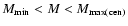
- Tinker et al. (2007) suggest a more physical model for
 that takes into account the scatter between mass and
luminosity. Tests comparing the simple model for
used in this work to their model, however, find no significant effect on the resulting correlation function.
that takes into account the scatter between mass and
luminosity. Tests comparing the simple model for
used in this work to their model, however, find no significant effect on the resulting correlation function.
- ... parameters
- In this case, values are chosen to correspond roughly to the best-fit parameter values found for the observed sample.
- ... Mpc
- The power-law slope
 for the cross-correlation is calculated by fitting for
 .
.
All Tables
Table 1: Number densities of volume-limited samples of SDSS galaxies.
Table 2: HOD parameters for mock data sets.
Table 3: Unmarginalized, best-fit parameters for mock data sets.
Table 4:
Unmarginalized, best-fit f and
![]() for mock data sets.
for mock data sets.
Table 5: HOD parameters for SDSS luminosity-threshold samples.
Table 6:
Unmarginalized, best-fit parameters for SDSS data using best-fit
![]() .
.
Table 7:
Unmarginalized, best-fit parameters for SDSS data varying
![]() .
.
All Figures
| |
Figure 1: The measured projected correlation functions in the SDSS data, where the cross-correlation of bright and faint galaxies is indicated by filled circles, the bright autocorrelation by open circles, and the faint autocorrelation by filled triangles. Bright galaxies have r-band magnitudes between -21 and -20, while faint galaxies have r-band magnitudes between -19 and -18. |
| Open with DEXTER | |
| In the text | |
| |
Figure 2:
The 68 and 90% marginalized confidence intervals are shown for pairs of parameters in the idealized data set. All masses are shown in log(
|
| Open with DEXTER | |
| In the text | |
| |
Figure 3: Top: the estimated cross-correlation ( circles) compared to the halo model cross-correlation using the best-fit HOD parameters ( solid line). Bottom: the shape of the HOD for the bright sample ( dotted) and the faint sample ( solid). |
| Open with DEXTER | |
| In the text | |
| |
Figure 4:
The normalized, marginalized likelihoods for all parameters (M1, |
| Open with DEXTER | |
| In the text | |
Copyright ESO 2009
Current usage metrics show cumulative count of Article Views (full-text article views including HTML views, PDF and ePub downloads, according to the available data) and Abstracts Views on Vision4Press platform.
Data correspond to usage on the plateform after 2015. The current usage metrics is available 48-96 hours after online publication and is updated daily on week days.
Initial download of the metrics may take a while.