


| Issue |
A&A
Volume 710, June 2026
|
|
|---|---|---|
| Article Number | A224 | |
| Number of page(s) | 7 | |
| Section | Galactic structure, stellar clusters and populations | |
| DOI | https://doi.org/10.1051/0004-6361/202660189 | |
| Published online | 12 June 2026 | |
Gaia-Sausage-Enceladus: Lithium evolution from early red-giant-branch and main-sequence stars
1
Department of Physics, University of Trieste,
Piazzale Europa, 1,
Trieste,
Italy
2
INAF – Osservatorio Astronomico di Trieste,
Via Giambattista Tiepolo, 11,
Trieste,
Italy
3
Institut für Astronomie und Astrophysik, Eberhard Karls Universität Tübingen,
Sand 1,
72076
Tübingen,
Germany
4
INAF, Osservatorio Astrofisico di Arcetri,
Largo E. Fermi 5,
50125
Firenze,
Italy
5
Department of Physics and Astronomy, Uppsala University,
Box 516,
75120
Uppsala,
Sweden
★ Corresponding author: This email address is being protected from spambots. You need JavaScript enabled to view it.
Received:
1
April
2026
Accepted:
20
May
2026
Abstract
The combination of data from the Gaia satellite and large ground-based spectroscopic surveys recently led to a milestone understanding of our Galaxy’s formation history, marked by the identification of stellar remnants of the accreted Gaia-Sausage-Enceladus (GSE) dwarf galaxy. Lithium (Li) remains one of the most difficult elements to explain because of its complex behaviour over evolutionary timescales: both the Spite plateau observed in metal-poor main-sequence (MS) stars and the recently discovered Li plateau of early red-giant-branch (eRGB) stars in the Milky Way challenge current galactic chemical evolution models. In this article, we investigate the viability of these Li-plateau features in the GSE galaxy, using public data from current big surveys: GALAH, Gaia-ESO, and the collective SAGA database. We present a chemical evolution model of Li for GSE and find agreement with the observed data. We find the signature of Li plateau at low metallicities in both eRGB and MS stars. At higher metallicities, we see candidates of Li-enriched stars that have their main contribution from nova explosions. These results reinforce the universality of the Spite plateau, and indicate that the eRGB Li plateau might also be a universal feature across different galactic systems. A hint of a low nova Li yield in GSE is suggested by our eRGB sample from GALAH. However, the lack of stars at high metallicities, possibly caused by the merger event, prevents a precise study of nova contributions, and we expect that upcoming data will enable a more comprehensive analysis.
Key words: stars: abundances / galaxies: abundances / galaxies: evolution
© The Authors 2026
 Open Access article, published by EDP Sciences, under the terms of the Creative Commons Attribution License (https://creativecommons.org/licenses/by/4.0), which permits unrestricted use, distribution, and reproduction in any medium, provided the original work is properly cited.
This article is published in open access under the Subscribe to Open model. This email address is being protected from spambots. You need JavaScript enabled to view it. to support open access publication.
1 Introduction
Mergers with nearby galaxies have affected the structure and formation of the Milky Way (MW), which is formed via two main processes: in situ formation and accretion. While in situ stars were formed within the main body of the MW, accreted stars originated from nearby galaxies and were incorporated into it over time (Deason et al. 2016). The most prominent event is the major merger of the Gaia-Sausage- Enceladus (GSE) dwarf galaxy that occurred roughly 10 Gyr ago (Helmi et al. 2018). Thanks to the astrometric data from Gaia (Gaia Collaboration 2016) and the spectroscopic survey Apache Point Observatory Galactic Evolution Experiment (APOGEE; Majewski et al. 2017), the identification of substructures in the MW stellar halo led to a profound discovery of the GSE stellar populations (Helmi et al. 2018; Belokurov et al. 2018; Myeong et al. 2019). This merger event perturbed the formation and evolution of the MW (Carrillo et al. 2026). Hence, it is crucial to understand the formation history of the GSE progenitor. Historically, Nissen & Schuster (2010) was the first to identify two distinct halo populations with high- and low-[$a/Fe] sequences, of which the lower [$a/Fe] sequence was argued to be an accreted population. This was later confirmed by the discovery of GSE. Since then, many studies have delved into the reconstruction of GSE star formation history using its stellar abundances (e.g. Vincenzo et al. 2019; Hasselquist et al. 2021). Recently, by comparing the evolution of Mg, Fe, Ba, and Eu with that of the Sculptor and Fornax galaxies, Ernandes et al. (2024) suggested that GSE underwent a slow gas-enrichment first, followed by a star formation phase, and was then quenched by the merger. The metallicity range of GSE remnants is usually between −3 ≤ [Fe/H] ≤ −0.6, with the metallicity distribution function (MDF) peaking at [Fe/H] ≈-1.2 (Feuillet et al. 2021; Limberg et al. 2022).
Lithium (Li) is a fragile element, easily destroyed in the stellar interior at ~2.5× 10⁶ K (Pinsonneault 1997). Observations of warm and metal-poor main-sequence (MS) halo stars reveal a Li plateau, known as the Spite plateau (Spite & Spite 1982), with an average abundance of A(Li) ≈ 2.2 dex. In contrast, standard Big Bang nucleosynthesis predictions (Coc et al. 2014), assuming the cosmological parameters of Planck Collaboration XVI (2014), yield a higher primordial value, A(Li) ≈ 2.7 dex, leading to the well-known ‘cosmological Li problem’. Stellar internal processes certainly play a role, as the stars we observe today have evolved over the past 10-12Gyr (Korn et al. 2007; Fu et al. 2015; Gao et al. 2020). Meanwhile, stars at the solar neighbourhood metallicity show a complex pattern of Li enrichment and depletion that may originate from many sources; for example, cosmic rays (Prantzos 2012), nova explosions (Cescutti & Molaro 2019), stellar mixing processes (Borisov et al. 2024), and intrinsic properties (Dantas et al. 2025). These features make Li one of the most interesting elements with which to study galactic chemical evolution (see Charbonnel & Prantzos 2026, for a more thorough review).
Recent study by Nguyen et al. (2025b, hereafter Paper I) implemented corrections from stellar evolution as a possible explanation to the cosmological Li problem, and for the first time used early red-giant-branch (eRGB) stars to study Galactic Li evolution. Accordingly, chemical evolution model traces the evolution of an element in the interstellar medium. For Li, which is easily destroyed during the evolution of stars, a correction due to stellar evolution, is thus embedded into the model to reproduce the abundances observed in stars at different evolutionary phases.
Moreover, literature has confirmed the universality of the Spite plateau observed in MS stars in different galactic systems (e.g. Monaco et al. 2010; Nissen & Schuster 2012; Molaro et al. 2020a; Simpson et al. 2021). In this article, we first investigate the presence of the eRGB Li plateau in the GSE, and second present a galactic chemical evolution model for Li of the GSE. We adopt the available data from the Galactic Archaeology with HERMES survey (GALAH, De Silva et al. 2015), complemented by data from the SAGA database (Suda et al. 2008) and the Gaia-ESO survey (Gilmore et al. 2012). Details of the selection method for GSE members are described in Sect. 2. In Sect. 3, we present a chemical evolution model for GSE. The obtained results are shown in Sect. 4, and we conclude this paper in Sect. 5.
2 Sample selection and kinematics
To study the Li evolution of GSE, we used data from the three catalogues GALAH DR3 (Wang et al. 2024), SAGA (Suda et al. 2008), and Gaia -ESO (Magrini et al. 2021). We selected the GSE members using the kinematic selection criteria defined by Feuillet et al. (2021), i.e. an angular momentum perpendicular to the galactic plane of −500 ≤ Lz (kpc km s−1) ≤500, and a radial action of  (the so-called Lz-Jr method).
For stars in the GALAH DR3 catalogue, we adopted the heliocentric co-ordinates and space velocities from Buder et al. (2021). In the SAGA and Gaia-ESO catalogues, these values are not provided and have to be computed. First, we sought the astrometric parameters from Gaia DR3 (Gaia Collaboration 2023) by querying at CDS using star identification included in these catalogues. For radial velocities, we adopted the values provided in these catalogues if available, and from Gaia DR3 otherwise. Then, we computed the co-ordinates and space velocities from the astrometric parameters with the transformations outlined in Sect. 4.1.7.1 of Hobbs et al. (2022).
We computed the orbital parameters with the Python package GALPY (Bovy 2015). To be consistent with Feuillet et al. (2021), we used the MWPOTENTIAL2014 package and Stäckel approximation (Binney 2012), adopting the same distance of the Sun to the Galactic centre, R⊙ = 8.0kpc (Bovy et al. 2012), its vertical offset to the Galactic plane, Z⊙ = 25 pc (Juric et al. 2008), as well as the space velocities of (U, V, W)⊙ = (11.1,12.24,7.25) km/s (Schönrich et al. 2010), with a local standard of rest of VLSR = 220 km/s (Bovy et al. 2012). Using the kinematic Lz-Jr selection method, we obtained 1257 stars from the GALAH DR3 catalogue (with high quality: flag_fe_h=0 and flag_sp=0), 32 stars from SAGA, and 8 stars from Gaia -ESO that belong to the GSE system. The stellar parameters, Li abundance, and kinematic properties of these stars are listed in Tables A.1 and A.2.
We further selected the samples of MS and eRGB stars by applying conditions to Teff and log g. In particular, we selected stars within 5800 ≤ Teff (K) ≤ 6900 and 3.8 ≤ log g (cms−2) ≤ 4.5 for our MS sample. For the eRGB stars, we defined a synthetic line along the RGB phase within a narrow range of 4800 ≤ Teff ≤ 5200 and 2.4 ≤ log g ≤ 3.3. Then, we selected stars within the range of  K for our eRGB sample. These choices of Teff and log g are to avoid stars undergoing Li depletion due to convective driven and thermohaline mixing. The Kiel and A(Li) vs. log g diagrams of stars in the two samples are shown in Fig. 1.
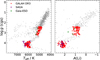 |
Fig. 1 Samples of MS and eRGB stars of GSE from the GALAH, SAGA, and Gaia-ESO catalogues. Left panel: Kiel diagram. Right panel: variation in A(Li) along with log g. The full sample of GSE from the GALAH catalogue is shown in the background (grey dots). |
3 Chemical evolution model
In this article, we used the concept introduced in our previous work (Paper I), which takes into account corrections to surface Li from stellar evolution, to study the Li evolution of GSE,
 (1)
(1)
The second term in Eq. (1), ΔA(Li)SM, is the correction due to stellar evolution. Similar to our previous work (for studying the Li evolution of the MW’s thin disc), we adopted the grids of stellar corrections for surface Li from Nguyen et al. (2025a). The correction term is ultimately dependent on metallicity, since we adopted the empirical mass-metallicity relations in Paper I. More details on deriving ΔA(Li)SM can be found in Appendix B.
The first term, A(Li)CEM, is the prediction from chemical evolution model. In this article, we adopted an infall model and assumed a Gaussian infall rate to describe the accreted gas to form the GSE galaxy (Cescutti et al. 2013). The infall rate is given by
 (2)
(2)
Here, MGSE is the total mass density of gas accreted into GSE, τ is the central peak of the infall distribution, and σ is the standard deviation of the infall law. The star formation rate (SFR) follows Schmidt’s law (Schmidt 1959), which is proportional to the surface gas density (see also Portinari & Chiosi 1999), ψ(t) = vSFRΣ(t)k, if the evolutionary time of the GSE has not yet reached a threshold value, parametrised as Tsfr. This value is set to the time when the GSE stops forming stars because of the interaction with the MW. As the evolutionary time goes beyond Tsfr, the SFR of the GSE is set to zero. In the expression above, vSFR is the efficiency coefficient of the SFR, Σ(t) is the total surface mass density of gas in GSE, and the exponential coefficient is k = 1.5 following Kennicutt (1998). Due to the interaction with the MW, an outflow wind operates for a period of time. In our model, the outflow wind rate is assumed to be proportional to the SFR, W(t) = νwindψ(t), with νwind as the wind efficiency coefficient. The time when the wind starts is characterised by Twind, and before this time the outflow wind rate is set to zero.
In total, our chemical evolution model has seven free parameters: MGSE, τ, σ, vSFR, Tsfr, vwind, and Twind. The first calibration of these parameters was done in Cescutti et al. (2020) using the APOGEE data. In this article, we recalibrated these parameters using GALAH DR3 data. We stress that, in order to reduce the number of free parameters, we assumed that GSE stopped forming stars at Tsfr ~ 7 Gyr ago. We then computed several models with given values of the other six parameters and relied on metallicity distribution function (MDF) to search for the best-fit values. In particular, the parameter space of these six parameters is summarised in Table 1. The normalised χ2 method was used to find the best match to the observed MDF. We collected the fits with χ2 ≤ 1 as our best-match models, and computed the mean values from the obtained results for each parameters. The best constrained values are listed in Table 1. The MDF predicted by our model, computed with the best constrained values, is shown in Fig. 2 and superimposed on the observed MDF of GSE. Moreover, we assumed that the ISM’s Li abundance is the cosmological value (A(Li) = 2.69 dex; Coc et al. 2014) in our calculations.
Furthermore, Li enrichment in the solar vicinity is explained by the contribution of Li produced by novae. We adopted the prescription of Cescutti & Molaro (2019) to take into account their contribution. Here, we adopted the delay time between when the primary star became a white dwarf and the nova explosion takes place, τnova= 1 Gyr; we also adopted a mean nova Li yield, LiYnova = 2.02 × 10⁻⁵M⊙, which was computed from observational data of Li production per nova event in the literature (Tajitsu et al. 2015; Molaro et al. 2016; Tajitsu et al. 2016; Izzo et al. 2018; Molaro et al. 2020b; Arai et al. 2021; Molaro et al. 2022, 2023; Izzo et al. 2025). We should clarify that an assumption that all novae produce the same amount of Li in all events is adopted in our model, together with a typical number of 104 outburst events over their entire lifetime (Ford 1978). A computed model without any stellar Li depletion is shown by the pink line in Fig. 3 for later comparisons.
Computed values of the six free parameters and their best-constrained values.
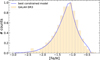 |
Fig. 2 MDF of GSE star members. Data were taken from the GALAH DR3 catalogue, binned in 0.1 dex of [Fe/H]. The displayed model was computed using the best-constrained values of the six parameters in Table 1. |
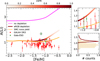 |
Fig. 3 Li evolution of the eRGB stars. Left panel: Model with Li depletion and LiYnova = 2.02 ×10⁻⁵M⊙ is colour-coded by the normalised SFR, while the model with LiYnova = 3.7 × 10⁻⁶M⊙ is shown by the orange line. A possible outlier star is circled in grey. Upper right panel: Zoom-in to the region of −1.05 ≤ [Fe/H] ≤ −0.75 of the left panel. Bottom right panel: Stellar distribution in Li abundance. |
4 Results and discussion
After constraining the free parameters using the MDF, we computed the chemical evolution model for Li assuming the original A(Li) = 2.69 dex and applied the correction term to take into account the Li depletion. Additional processes such as rotational mixing and angular momentum transport are expected to further enhance the Li depletion (Eggenberger et al. 2022), and intrinsic stellar properties may also contribute to the observed scatter (Dantas et al. 2025). As these effects are currently not included in the stellar correction term, our models preferentially trace the upper envelope of the evolutionary trend, explaining a small but systematic offset in the stellar distribution (Fig. 3, bottom panel).
In Fig. 3 (left panel), we show the 82 eRGB stars of GSE selected from the GALAH DR3 catalogue. It reveals a Li plateau at low metallicities, [Fe/H] ≤ −1.2, with a mean value of A(Li) = 0.914 dex and a standard deviation of 0.15 dex, which overlaps with the previous finding of Mucciarelli et al. (2022). The Mucciarelli et al. (2022) Li plateau was discovered among 58 field halo eRGB stars with high-solution spectra, and was reproduced by a Galactic thin disc chemical evolution model in Paper I. In this work, our model including the depletion correction up to the RGB bump is shown as the line coloured by the normalised SFR, indicating a Li-plateau feature at this metal-licity range, with an average A(Li) ≈ 1.1 dex. It is in agreement with the upper end of Li data from the GALAH sample. The predicted value is also consistent with the result of Paper I and the observed plateau in Mucciarelli et al. (2022). This result implies that the eRGB Li plateau may also be a universal feature across different galactic systems.
Novae are thought to play a dominant role in explaining the Li enrichment in the solar vicinity (e.g. Cescutti & Molaro 2019; Kemp et al. 2024). However, after the major merger event with the MW, GSE eventually stopped forming stars at some time, possibly Tsfr ≈ 7 Gyr ago as we assumed in this work. This prevents the formation of younger stars that are potentially enriched in Li by the former nova explosions. As a result, fewer GSE stars are found in the solar neighbourhood towards higher metallici-ties, preventing us from having a better constraint on the nova Li yield. Regardless, we computed our model with an average Li yield of L1Ynova = 2.02×10⁻⁵M⊙ as constrained from the novae observations. Among the GALAH catalogue, at [Fe/H] > -1.05 region, we find that the three most Li-rich stars align with the prediction of our model (see Fig. 3, upper right panel). Two of these stars, with [Fe/H]~ −1, are located at the rising base of the enrichment evolution. The other star, [Fe/H] ≈ −0.8, lies below our model prediction with an offset of ~ 0.07 dex (including the observed uncertainty). We also show in Fig. 3 three eRGB stars obtained from the Gaia-ESO catalogue. Two of these stars show their abundances at the rising base of the enrichment evolution. The other star shows a relatively high Li abundance in comparison with other star members, marked by the grey circle. It has A(L1)=1.68 dex, about 0.6 dex higher than the value reported by Mucciarelli et al. (2022). We notice that its radial action, √JR = 30.08 (kpc km s−1)1/2, lies at the border of our selection criterion. This raises questions about its membership. Moreover, the existence of Li-rich giants (e.g. Smiljanic et al. 2018) further complicates the interpretation of its nature. We therefore consider it an outlier in this paper. The agreement between our model predictions and the Li abundances of these stars may help constrain the nova Li yield in GSE. However, they are mostly at the rising base of the enrichment evolution, preventing a firm conclusion on the adopted yield.
In addition, within the GALAH sample, a relatively flat trend can be depicted in our eRGB stars. This may suggest that GSE exhibits a lower nova Li yield. We include a model adopting the observed Li production per nova event of the Small Magellanic Cloud (SMC; Izzo et al. 2022), yielding LiYnova = 3.7 × 10⁻⁶ M⊙, in Fig. 3 (orange line). The MDF of the SMC peaks at [Fe/H] ~ −1 (Mucciarelli et al. 2023), which is similar to the GSE metal-licity. Our model with a low nova Li yield tends to reproduce the flat tendency in eRGB stars, but is quite low to reproduce the most Li-rich stars. We should stress that a nova Li yield should depend on stellar mass and metallicity, and that more work is needed to capture the full complexity of chemical enrichment from a population of novae, particularly for the GSE, where stars at higher metallicities are lacking (see Kemp et al. 2022, for more discussion).
The Spite plateau found in the MW had also been suggested as a common feature in other galaxies (e.g. Monaco et al. 2010). Likewise, Molaro et al. (2020a) (hereafter, MCF20) drew a similar conclusion on GSE by adopting data from the GALAH DR2 and SAGA catalogues, aligning with the conclusions of Nissen & Schuster (2012). However, MCF20 determined the GSE members by cross-matching with the former determination of Helmi et al. (2018). In this regard, we recall that we used the new definition of Feuillet et al. (2021) to determine the memberships of the GSE (Sect. 2). Due to differences in the definition, we find only 15 stars in our SAGA sample present in the MCF20 sample. Regardless of this limited overlap, we find agreement with MCF20 on the Spite plateau in GSE. In particular, at [Fe/H] < -1.4, our model shows an excellent fit to the observed data, especially of SAGA (Fig. 4, left panel), with a predicted A(Li) ≈ 2.14-2.31 dex. Our data at this metallicity range from the GALAH sample indicate a mean Li abundance of A(Li) = 2.2 dex and a standard deviation of 0.14 dex. Furthermore, Simpson et al. (2021) applied the same GSE selection method to the GALAH DR3 data (Buder et al. 2021) and found that GSE indeed exhibits the same Li plateau (A(Li) = 2.35 ± 0.12 dex) as other accreted and in situ MW stars. This result and the agreement with other studies once again reinforces the universality hypothesis of the Spite plateau across different galactic systems (see also Matteucci et al. 2021).
Similarly to the case of eRGB stars, we could not fully study the contribution of novae at the enrichment evolution by using MS stars. We find only two stars at [Fe/H]~ −1, each from one catalogue, located at the rising base of the enrichment branch. Nonetheless, our model, adopting the mean value of observed nova Li yields, predicts the abundances of these two stars very well. The most metal-rich star from the GALAH sample in Fig. 4 shows a Li abundance that can be reproduced by lowering the nova Li yield, as indicated by our model with a yield of the SMC. However, radial action of this star,  = 30.3(kpckms−1)1/2, raises questions about its membership. Therefore, we do not rely on this star in our current calibration. In this regard, we note that current and ongoing large surveys are rapidly improving in terms of both data precision and sample size. We thus remain optimistic about more robust studies in the future.
Additionally, we should clarify that the GALAH DR4 catalogue (Buder et al. 2025) recently released a larger sample of stars. However, the catalogue has a problem in flagging [Fe/H], so we cannot select stars with a good determination of the iron abundance. For this reason, we chose to adopt data from the GALAH DR3 catalogue in this work. A tentative test using GALAH DR4 data can be found in Appendix C. In general, we see similar trends in the A(Li) versus [Fe/H] diagram between the two catalogues.
5 Summary and conclusions
The CEM of Li in a dwarf galaxy is expected to be different from that of the MW. In this context, the accreted GSE stars offer a unique opportunity to study Li evolution in a dwarf galaxy, since dwarf galaxies are often distant and their stellar Li abundances are difficult to measure. We adopted the available data from recent and current big surveys: GALAH DR3, Gaia-ESO, and the SAGA database, and used the Lz-Jr method to determine GSE membership. We then presented the Li evolution models for GSE and compared them with the observed data to study the Li plateaus in the MS and eRGB phases. The results reinforce the universality of the Spite plateau and suggest that the eRGB Li plateau may also be universal across different galactic systems. This opens a new category of observational targets for galactic Li evolution studies, since eRGB stars are significantly brighter and easier to observe at high resolution than near-MS stars. Our model also leads to a hint that GSE may exhibit a low nova Li yield, and that improvements in both the modelling of nova contributions and data sample would help us to draw more robust conclusions about this matter. To conclude this article, we present in Tables A.1 and A.2 the stellar parameters and kinematic information of GSE stars determined in this paper, available at a Zenodo repository1.
Acknowledgements
We are grateful for the kind and constructive comments and suggestions from the referee, especially on the discussion of nova Li yield. This certainly strengthens our paper. CTN, GC, LM acknowledge the financial support under the National Recovery and Resilience Plan (NRRP), Mission 4, Component 2, Investment 1.1, Call for tender No. 104 published on 2.2.2022 by the Italian Ministry of University and Research (MUR), funded by the European Union - NextGenerationEU - Project ‘Cosmic POT’ (PI: L. Magrini) Grant Assignment Decree No. 2022X4TM3H by the Italian Ministry of Ministry of University and Research (MUR). CTN, GC, AK acknowledge funding from the European Union’s Horizon 2020 research and innovation programme under grant agreement No. 101008324 (ChETEC-INFRA). CTN, GC acknowledge the support by INAF Mini grant 2024, “GALoMS - Galactic Archaeology for Low Mass Stars” (1.05.24.07.02). AJK acknowledges support by the Swedish National Space Agency (SNSA). The authors gratefully acknowledge the works behind the Gaia mission, ground-based spectroscopic surveys: GALAH, Gaia-ESO, and the collective SAGA database, for providing the data used in this work. This work also makes use of the TOPCAT software (Taylor 2005). CTN thanks Emanuele Spitoni, Alexandro Saro, Emma Dodd, Ella Xi Wang, Linda Lombardo and Umberto Maio for helpful discussions over the course of this work.
References
- Arai, A., Tajitsu, A., Kawakita, H., & Shinnaka, Y. 2021, ApJ, 916, 44 [Google Scholar]
- Asplund, M., Lambert, D. L., Nissen, P. E., Primas, F., & Smith, V. V. 2006, ApJ, 644, 229 [NASA ADS] [CrossRef] [Google Scholar]
- Belokurov, V., Erkal, D., Evans, N. W., Koposov, S. E., & Deason, A. J. 2018, MNRAS, 478, 611 [Google Scholar]
- Binney, J. 2012, MNRAS, 426, 1324 [Google Scholar]
- Boesgaard, A. M. 2007, ApJ, 667, 1196 [NASA ADS] [CrossRef] [Google Scholar]
- Bonifacio, P., & Molaro, P. 1997, MNRAS, 285, 847 [NASA ADS] [CrossRef] [Google Scholar]
- Bonifacio, P., Sbordone, L., Caffau, E., et al. 2012, A&A, 542, A87 [NASA ADS] [CrossRef] [EDP Sciences] [Google Scholar]
- Borisov, S., Charbonnel, C., Prantzos, N., Dumont, T., & Palacios, A. 2024, A&A, 690, A245 [NASA ADS] [CrossRef] [EDP Sciences] [Google Scholar]
- Bovy, J. 2015, ApJS, 216, 29 [NASA ADS] [CrossRef] [Google Scholar]
- Bovy, J., Allende Prieto, C., Beers, T. C., et al. 2012, ApJ, 759, 131 [NASA ADS] [CrossRef] [Google Scholar]
- Buder, S., Sharma, S., Kos, J., et al. 2021, MNRAS, 506, 150 [NASA ADS] [CrossRef] [Google Scholar]
- Buder, S., Kos, J., Wang, X. E., et al. 2025, PASA, 42, e051 [Google Scholar]
- Carrillo, A., Deason, A. J., Fattahi, A., Grand, R. J. J., & Fragkoudi, F. 2026, MNRAS, 546, stag111 [Google Scholar]
- Cescutti, G., & Molaro, P. 2019, MNRAS, 482, 4372 [NASA ADS] [CrossRef] [Google Scholar]
- Cescutti, G., Chiappini, C., Hirschi, R., Meynet, G., & Frischknecht, U. 2013, A&A, 553, A51 [NASA ADS] [CrossRef] [EDP Sciences] [Google Scholar]
- Cescutti, G., Molaro, P., & Fu, X. 2020, Mem. Soc. Astron. Italiana, 91, 153 [NASA ADS] [Google Scholar]
- Charbonnel, C., & Prantzos, N. 2026, arXiv e-prints [arXiv:2602.17470] [Google Scholar]
- Coc, A., Uzan, J.-P., & Vangioni, E. 2014, JCAP, 2014, 050 [Google Scholar]
- Dantas, M. L. L., Smiljanic, R., Romano, D., et al. 2025, A&A, 699, A173 [NASA ADS] [CrossRef] [EDP Sciences] [Google Scholar]
- De Silva, G. M., Freeman, K. C., Bland-Hawthorn, J., et al. 2015, MNRAS, 449, 2604 [NASA ADS] [CrossRef] [Google Scholar]
- Deason, A. J., Mao, Y.-Y., & Wechsler, R. H. 2016, ApJ, 821, 5 [NASA ADS] [CrossRef] [Google Scholar]
- Eggenberger, P., Buldgen, G., Salmon, S. J. A. J., et al. 2022, Nat. Astron., 6, 788 [NASA ADS] [CrossRef] [Google Scholar]
- Ernandes, H., Feuillet, D., Feltzing, S., & Skúladóttir, Á. 2024, A&A, 691, A333 [NASA ADS] [CrossRef] [EDP Sciences] [Google Scholar]
- Feuillet, D. K., Sahlholdt, C. L., Feltzing, S., & Casagrande, L. 2021, MNRAS, 508, 1489 [NASA ADS] [CrossRef] [Google Scholar]
- Ford, H. C. 1978, ApJ, 219, 595 [Google Scholar]
- Fu, X., Bressan, A., Molaro, P., & Marigo, P. 2015, MNRAS, 452, 3256 [CrossRef] [Google Scholar]
- Gaia Collaboration (Prusti, T., et al.) 2016, A&A, 595, A1 [NASA ADS] [CrossRef] [EDP Sciences] [Google Scholar]
- Gaia Collaboration (Vallenari, A., et al.) 2023, A&A, 674, A1 [NASA ADS] [CrossRef] [EDP Sciences] [Google Scholar]
- Gao, X., Lind, K., Amarsi, A. M., et al. 2020, MNRAS, 497, L30 [Google Scholar]
- Gilmore, G., Randich, S., Asplund, M., et al. 2012, The Messenger, 147, 25 [NASA ADS] [Google Scholar]
- Hansen, C. J., Nordström, B., Bonifacio, P., et al. 2011, A&A, 527, A65 [NASA ADS] [CrossRef] [EDP Sciences] [Google Scholar]
- Hansen, T., Hansen, C. J., Christlieb, N., et al. 2014, ApJ, 787, 162 [NASA ADS] [CrossRef] [Google Scholar]
- Hansen, T., Hansen, C. J., Christlieb, N., et al. 2015, ApJ, 807, 173 [Google Scholar]
- Hasselquist, S., Hayes, C. R., Lian, J., et al. 2021, ApJ, 923, 172 [NASA ADS] [CrossRef] [Google Scholar]
- Helmi, A., Babusiaux, C., Koppelman, H. H., et al. 2018, Nature, 563, 85 [Google Scholar]
- Hobbs, D., Lindegren, L., Bastian, U., et al. 2022, Gaia DR3 documentation, Chapter 4: Astrometric data [Google Scholar]
- Izzo, L., Molaro, P., Bonifacio, P., et al. 2018, MNRAS, 478, 1601 [NASA ADS] [CrossRef] [Google Scholar]
- Izzo, L., Molaro, P., Cescutti, G., et al. 2022, MNRAS, 510, 5302 [CrossRef] [Google Scholar]
- Izzo, L., Siegert, T., Jean, P., et al. 2025, A&A, 698, A291 [NASA ADS] [CrossRef] [EDP Sciences] [Google Scholar]
- Juric, M., Ivezic, Z., Brooks, A., et al. 2008, ApJ, 673, 864 [Google Scholar]
- Kemp, A. J., Karakas, A. I., Casey, A. R., Kobayashi, C., & Izzard, R. G. 2022, MNRAS, 509, 1175 [Google Scholar]
- Kemp, A. J., Karakas, A. I., Casey, A. R., et al. 2024, A&A, 689, A222 [NASA ADS] [CrossRef] [EDP Sciences] [Google Scholar]
- Kennicutt, Jr., R. C. 1998, ApJ, 498, 541 [Google Scholar]
- Korn, A. J., Grundahl, F., Richard, O., et al. 2007, ApJ, 671, 402 [NASA ADS] [CrossRef] [Google Scholar]
- Li, H., Aoki, W., Matsuno, T., et al. 2018, ApJ, 852, L31 [NASA ADS] [CrossRef] [Google Scholar]
- Limberg, G., Souza, S. O., Pérez-Villegas, A., et al. 2022, ApJ, 935, 109 [NASA ADS] [CrossRef] [Google Scholar]
- Magrini, L., Lagarde, N., Charbonnel, C., et al. 2021, A&A, 651, A84 [NASA ADS] [CrossRef] [EDP Sciences] [Google Scholar]
- Majewski, S. R., Schiavon, R. P., Frinchaboy, P. M., et al. 2017, AJ, 154, 94 [NASA ADS] [CrossRef] [Google Scholar]
- Masseron, T., Johnson, J. A., Lucatello, S., et al. 2012, ApJ, 751, 14 [NASA ADS] [CrossRef] [Google Scholar]
- Matteucci, F., Molero, M., Aguado, D. S., & Romano, D. 2021, MNRAS, 505, 200 [NASA ADS] [CrossRef] [Google Scholar]
- Meléndez, J., Casagrande, L., Ramírez, I., Asplund, M., & Schuster, W. J. 2010, A&A, 515, L3 [NASA ADS] [CrossRef] [EDP Sciences] [Google Scholar]
- Molaro, P., Izzo, L., Mason, E., Bonifacio, P., & Della Valle, M. 2016, MNRAS, 463, L117 [NASA ADS] [CrossRef] [Google Scholar]
- Molaro, P., Cescutti, G., & Fu, X. 2020a, MNRAS, 496, 2902 [Google Scholar]
- Molaro, P., Izzo, L., Bonifacio, P., et al. 2020b, MNRAS, 492, 4975 [NASA ADS] [CrossRef] [Google Scholar]
- Molaro, P., Izzo, L., D’Odorico, V., et al. 2022, MNRAS, 509, 3258 [Google Scholar]
- Molaro, P., Izzo, L., Selvelli, P., et al. 2023, MNRAS, 518, 2614 [Google Scholar]
- Molaro, P., Bonifacio, P., Cupani, G., & Howk, J. C. 2024, A&A, 690, A38 [NASA ADS] [CrossRef] [EDP Sciences] [Google Scholar]
- Monaco, L., Bonifacio, P., Sbordone, L., Villanova, S., & Pancino, E. 2010, A&A, 519, L3 [NASA ADS] [CrossRef] [EDP Sciences] [Google Scholar]
- Mucciarelli, A., Monaco, L., Bonifacio, P., et al. 2022, A&A, 661, A153 [NASA ADS] [CrossRef] [EDP Sciences] [Google Scholar]
- Mucciarelli, A., Minelli, A., Bellazzini, M., et al. 2023, A&A, 671, A124 [NASA ADS] [CrossRef] [EDP Sciences] [Google Scholar]
- Myeong, G. C., Vasiliev, E., Iorio, G., Evans, N. W., & Belokurov, V. 2019, MNRAS, 488, 1235 [Google Scholar]
- Nguyen, C. T., Bressan, A., Korn, A. J., et al. 2025a, A&A, 696, A136 [NASA ADS] [CrossRef] [EDP Sciences] [Google Scholar]
- Nguyen, C. T., Cescutti, G., Matteucci, F., et al. 2025b, A&A, 703, A204 [NASA ADS] [CrossRef] [EDP Sciences] [Google Scholar]
- Nissen, P. E., & Schuster, W. J. 2010, A&A, 511, L10 [NASA ADS] [CrossRef] [EDP Sciences] [Google Scholar]
- Nissen, P. E., & Schuster, W. J. 2012, A&A, 543, A28 [NASA ADS] [CrossRef] [EDP Sciences] [Google Scholar]
- Pinsonneault, M. 1997, ARA&A, 35, 557 [Google Scholar]
- Planck Collaboration XVI. 2014, A&A, 571, A16 [NASA ADS] [CrossRef] [EDP Sciences] [Google Scholar]
- Portinari, L., & Chiosi, C. 1999, A&A, 350, 827 [NASA ADS] [Google Scholar]
- Prantzos, N. 2012, A&A, 542, A67 [NASA ADS] [CrossRef] [EDP Sciences] [Google Scholar]
- Richard, O., Michaud, G., & Richer, J. 2005, ApJ, 619, 538 [Google Scholar]
- Sakari, C. M., Placco, V. M., Farrell, E. M., et al. 2018, ApJ, 868, 110 [Google Scholar]
- Sbordone, L., Bonifacio, P., Caffau, E., et al. 2010, A&A, 522, A26 [NASA ADS] [CrossRef] [EDP Sciences] [Google Scholar]
- Schmidt, M. 1959, ApJ, 129, 243 [NASA ADS] [CrossRef] [Google Scholar]
- Schönrich, R., Binney, J., & Dehnen, W. 2010, MNRAS, 403, 1829 [NASA ADS] [CrossRef] [Google Scholar]
- Simpson, J. D., Martell, S. L., Buder, S., et al. 2021, MNRAS, 507, 43 [NASA ADS] [CrossRef] [Google Scholar]
- Smiljanic, R., Pasquini, L., Bonifacio, P., et al. 2009, A&A, 499, 103 [NASA ADS] [CrossRef] [EDP Sciences] [Google Scholar]
- Smiljanic, R., Franciosini, E., Bragaglia, A., et al. 2018, A&A, 617, A4 [NASA ADS] [CrossRef] [EDP Sciences] [Google Scholar]
- Spite, M., & Spite, F. 1982, Nature, 297, 483 [NASA ADS] [CrossRef] [Google Scholar]
- Suda, T., Katsuta, Y., Yamada, S., et al. 2008, PASJ, 60, 1159 [NASA ADS] [Google Scholar]
- Tajitsu, A., Sadakane, K., Naito, H., Arai, A., & Aoki, W. 2015, Nature, 518, 381 [NASA ADS] [CrossRef] [Google Scholar]
- Tajitsu, A., Sadakane, K., Naito, H., et al. 2016, ApJ, 818, 191 [NASA ADS] [Google Scholar]
- Tan, K. F., Shi, J. R., & Zhao, G. 2009, MNRAS, 392, 205 [Google Scholar]
- Taylor, M. B. 2005, in Astronomical Society of the Pacific Conference Series, 347, Astronomical Data Analysis Software and Systems XIV, eds. P. Shopbell, M. Britton, & R. Ebert, 29 [Google Scholar]
- Vincenzo, F., Spitoni, E., Calura, F., et al. 2019, MNRAS, 487, L47 [NASA ADS] [CrossRef] [Google Scholar]
- Wang, E. X., Nordlander, T., Buder, S., et al. 2024, MNRAS, 528, 5394 [CrossRef] [Google Scholar]
- Yang, W., Dou, S., Meng, X., Wu, Y., & Bi, S. 2026, ApJ, 1000, 271 [Google Scholar]
Appendix A Table
Here we present the stellar parameters and Li abundances of 32 stars from the collective SAGA database, along with their references in Table A.1. Meanwhile, for stars from the GALAH (Wang et al. 2024) and Gaia-ESO (Magrini et al. 2021) catalogues, we refer readers to the original catalogues for these properties. In Table A.2, we summarise the kinematic and orbital properties of all GSE stars from three catalogues, determined in this article. These two tables can be found at the mentioned Zenodo repository1.
Stellar parameters and Li abundances of 32 stars from the SAGA database that belong to the GSE. The last column reports references.
Appendix B The stellar correction term
We here summarise the derivation of ΔA(Li)SM in Eq. 1. The term is computed from grids of stellar tracks, providing the Li depletion from initial value, reflecting Li abundance of the ISM, to a given evolutionary phase (e.g. the MS and eRGB phases).
First of all, it should be recalled that the CEM calculation traces the evolution of a given element in the interstellar medium (ISM; or the stellar birth cloud) across galactic lifetime. Details of CEM for GSE can be found in Sect. 3 of this paper. The Li abundance of ISM, whether cosmological (A(Li) ≈ 2.7 dex) or Spite plateau (A(Li) ≈ 2.2 dex) values, is a debatable subject still to date (see also Molaro et al. 2024). However, in this paper, we assume the Li abundance of ISM is the cosmological value and do not necessarily disown the other scenario, as we showed in Paper I.
For deriving ΔA(Li)SM in the eRGB phase, we adopt the stellar grid of Nguyen et al. (2025a) which includes two sets of tracks of metallicities, [Fe/H] = −2.4 and −2.1, and masses from 0.65 to 0.94M⊙. The predicted stellar-evolution correction is equal to the difference between the initial value in the beginning of the PMS phase and the value when the star reaches the Li-plateau value among RGB stars at a log g of ~ 2.8(cms−2). We should clarify that these tracks were computed with an initial A(Li) = 2.69 dex, consistent with the assumed A(Li) of ISM in our CEM, and subsequently depleted during the PMS phase so that they reach the Spite plateau value at the MS phase. The stellar model prediction was then calibrated to Li data of the globular cluster NGC 6397. Additionally, if the ISM is assumed to have the Spite plateau value, there would be no depletion during the PMS phase as definition. In this case, the predicted stellar-evolution correction is equal to the difference between the value in the MS phase and the value in the RGB phase as defined above. Finally, due to the limited range of metallicity, an extrapolation scheme was applied in case the galactic evolutionary metallicity exceeds the limits of the stellar grid.
A similar approach is applied to derive ΔA(Li)SM in the MS phase. In addition, we must emphasise that there are other mechanisms have been proposed to explain the cosmological Li problem by introducing different stellar extra-mixing prescriptions such as turbulent diffusion (Richard et al. 2005), late mass accretion during the PMS phase (Fu et al. 2015) or rotation and magnetic fields (Yang et al. 2026). Access to these stellar libraries would be valuable for deriving the stellar correction term in our CEM; however, we are at present limited in this regard.
Appendix C Analysis using GALAH DR4 data
In this appendix we redo our study in this work by using data from the GALAH DR4 catalogue (Buder et al. 2025). Overall, the sample size increases to 1842 stars, about 500 stars more than the sample using the GALAH DR3 catalogue. Fig. C.1 shows the obtained MDF, indicating an offset with our model prediction, or rather with the GALAH DR3 catalogue. This may be explained by the quality selection in iron abundances, i.e. we cannot select stars with flag_fe_h=0 due to a bug arose in the GALAH DR4. Works in progress to solve this problem and calibrations to further evaluate the new released data have been claimed to be provided in the future (see Buder et al. 2025). Regardless, we then make a tentative analysis on the Li evolution. The results are shown in Figs. C.2 and C.3. For the Li plateaus at low metal-licities, we obtain an agreement with our main results in Figs. 3 and 4. The nova Li contribution remains ambiguous.
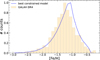 |
Fig. C.1 MDF of GSE by using the GALAH DR4 data. |
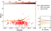 |
Fig. C.2 Li evolution in eRGB stars by using the GALAH DR4 data. |
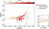 |
Fig. C.3 Li evolution in MS stars by using the GALAH DR4 data. |
All Tables
Stellar parameters and Li abundances of 32 stars from the SAGA database that belong to the GSE. The last column reports references.
All Figures
|
Fig. 1 Samples of MS and eRGB stars of GSE from the GALAH, SAGA, and Gaia-ESO catalogues. Left panel: Kiel diagram. Right panel: variation in A(Li) along with log g. The full sample of GSE from the GALAH catalogue is shown in the background (grey dots). |
| In the text | |
|
Fig. 2 MDF of GSE star members. Data were taken from the GALAH DR3 catalogue, binned in 0.1 dex of [Fe/H]. The displayed model was computed using the best-constrained values of the six parameters in Table 1. |
| In the text | |
|
Fig. 3 Li evolution of the eRGB stars. Left panel: Model with Li depletion and LiYnova = 2.02 ×10⁻⁵M⊙ is colour-coded by the normalised SFR, while the model with LiYnova = 3.7 × 10⁻⁶M⊙ is shown by the orange line. A possible outlier star is circled in grey. Upper right panel: Zoom-in to the region of −1.05 ≤ [Fe/H] ≤ −0.75 of the left panel. Bottom right panel: Stellar distribution in Li abundance. |
| In the text | |
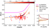 |
Fig. 4 Same as Fig. 3 but for the MS stars. |
| In the text | |
|
Fig. C.1 MDF of GSE by using the GALAH DR4 data. |
| In the text | |
|
Fig. C.2 Li evolution in eRGB stars by using the GALAH DR4 data. |
| In the text | |
|
Fig. C.3 Li evolution in MS stars by using the GALAH DR4 data. |
| In the text | |
Current usage metrics show cumulative count of Article Views (full-text article views including HTML views, PDF and ePub downloads, according to the available data) and Abstracts Views on Vision4Press platform.
Data correspond to usage on the plateform after 2015. The current usage metrics is available 48-96 hours after online publication and is updated daily on week days.
Initial download of the metrics may take a while.