


| Issue |
A&A
Volume 711, July 2026
|
|
|---|---|---|
| Article Number | A274 | |
| Number of page(s) | 6 | |
| Section | Astrophysical processes | |
| DOI | https://doi.org/10.1051/0004-6361/202659647 | |
| Published online | 21 July 2026 | |
Radio eclipse of the slowest spinning Galactic-field spider pulsar PSR J1932+2121 and its X-ray emission prospect
1
Institute of Astrophysics, Central China Normal University, Wuhan 430079, China
2
Laboratory for Compact Object Astrophysics and Astronomical Technology, Central China Normal University, Wuhan 430079, China
3
National Astronomical Observatories, Chinese Academy of Sciences, Jia-20 Datun Road ChaoYang District Beijing 100012, China
4
School of Astronomy and Space Science, University of Chinese Academy of Sciences, Beijing 100049, China
5
Key Laboratory of Radio Astronomy and Technology, Chinese Academy of Sciences, Beijing 100101, China
6
School of Physical Science and Technology, Southwest University, Chongqing 400715, China
★ Corresponding authors: This email address is being protected from spambots. You need JavaScript enabled to view it.
; This email address is being protected from spambots. You need JavaScript enabled to view it.
; This email address is being protected from spambots. You need JavaScript enabled to view it.
Received:
28
February
2026
Accepted:
9
June
2026
Abstract
PSR J1932+2121 is a newly discovered spider pulsar with a pronounced radio eclipse identified by the Five-hundred-meter Aperture Spherical radio Telescope (FAST); it provides an ideal laboratory for studying the eclipse mechanism and high-energy emission from its intrabinary shock (IBS). By modeling the orbital-phase-dependent dispersion measure variations and flux profiles during the eclipse region with the wind interaction and IBS geometry, we constrain the system to a nearly edge-on inclination (io ≃ 88.55°) and a weak stellar wind from a low-mass main-sequence companion. Our analysis of the eclipse mechanism suggests that synchrotron absorption by nonthermal electrons can reproduce the observed flux variations with reasonable parameters for the eclipsing medium. We further predict the synchrotron emission from the IBS in PSR J1932+2121, showing that its X-ray flux, particularly near the inferior conjunction of the companion star, could be detectable with XMM/EPIC, EP/FXT, or eXTP/SFA and should exhibit double-peaked orbital modulation by Doppler boosting. These results provide a theoretical framework for understanding this system and for guiding future multiwavelength probes of spider pulsars.
Key words: magnetic reconnection / radiation: dynamics / binaries: eclipsing / stars: winds / outflows
© The Authors 2026
 Open Access article, published by EDP Sciences, under the terms of the Creative Commons Attribution License (https://creativecommons.org/licenses/by/4.0), which permits unrestricted use, distribution, and reproduction in any medium, provided the original work is properly cited.
This article is published in open access under the Subscribe to Open model. This email address is being protected from spambots. You need JavaScript enabled to view it. to support open access publication.
1. Introduction
The Galactic Plane Pulsar Snapshot (GPPS) survey (Han et al. 2021) by the Five-hundred-meter Aperture Spherical radio Telescope (FAST) has discovered a large number of new pulsars; to date, 751 pulsars have been detected (Han et al. 2025). Approximately 20% of these exhibit characteristics consistent with binary systems (Wang et al. 2025), thus enabling more detailed studies of binary properties, evolutionary features, and population statistics (Koljonen & Linares 2025). Here, when the binary orbital plane is close to the direction of the line of sight (LOS) and the companion star moves near its inferior conjunction (INFC), the wind material from the companion is expected to obscure the radio emission of the pulsar, producing periodical eclipse features (Kluzniak et al. 1988; Stappers 1996; Guillemot et al. 2019; Nieder et al. 2020). The study of these eclipses provides valuable insight into the eclipse mechanism and probes the physical conditions of the binary environment (Phinney 1988; Thompson et al. 1994; Polzin et al. 2020; Miao et al. 2023).
In particular, when the pulsar is a millisecond pulsar (MSP), the companion star can be ablated significantly by pulsar irradiation (Fruchter et al. 1988; Khechinashvili et al. 2000; Chen et al. 2013; Koljonen & Linares 2025), finally becoming a low-mass star in tight, near-circular orbits. Such pulsar binaries are generally called spider pulsar binaries. More specifically, these systems are commonly subdivided into redbacks, with companion masses of ∼0.2 − 0.4M⊙, and black widows, whose companions are ultra-low mass, ∼0.02 − 0.05M⊙ (Roberts 2013; Polzin et al. 2019). The strong interaction between the winds of the pulsar and companion can form an intrabinary shock (IBS; e.g., bow shock), which significantly increases the chance of detecting an eclipse phenomenon (Wadiasingh et al. 2017; Du et al. 2023). Moreover, the resulting cometary structure of the IBS would directly govern the radio eclipse boundary.
In addition to radio eclipses, high-energy emission has also been detected from the interaction of the spider pulsar wind with the evaporating companion material (Ruderman et al. 1989; Huang & Becker 2007; Roberts et al. 2014; Karpova et al. 2025; Satybaldiev et al. 2026) as this emission can be naturally interpreted as synchrotron radiation from the IBS zone that is modulated by the orbital motion (Romani & Sanchez 2016; Wadiasingh et al. 2017; Kandel et al. 2019; de Martino et al. 2020; Sim et al. 2024). Therefore, a joint modeling of the radio eclipse and the IBS high-energy emission is essential for constraining the properties of the companion outflow, the wind interaction, and even the dynamical evolution of the pulsar wind.
Among the growing binary samples, a remarkable fraction have been identified as spider pulsars (Wang et al. 2025), including PSR J1932+2121, which was discovered in the FAST GPPS survey. PSR J1932+2121 is distinctive as the slowest spinning Galactic-field spider pulsar currently known, with a spin period of 14.25 ms, ultra-compact orbit, and pronounced radio eclipses. Therefore, this work was devoted to modeling the radio eclipses of this particular spider pulsar and to predicting its multiwavelength emission properties. The paper is organized as follows. In Sect. 2 we describe our observation with FAST and data processing. The flux and dispersion measure (DM) obtained from PSR J1932+2121 are presented. In Sect. 3 we revisit the eclipse model and constrain the parameters of the binary orbit and the companion star. In Sect. 4 we calculate the X-ray emission arising from the IBS with the obtained model parameters, where the dynamical evolution of the pulsar wind is taken into account. Finally, the implications for the eclipse mechanism and the intrabinary environment of PSR J1932+2121 are summarized in Sect. 5.
2. FAST observations of PSR J1932+2121
PSR J1932+2121 has a spin period of 14.25 ms and a spin-down luminosity of 4.8×1033 erg s−1 (Wang et al. 2025) and moves in a 1.94-hour orbit. The minimum mass of the companion is 0.115 M⊙, placing it among spider pulsars (Wang et al. 2025; Han et al. 2025; Misra et al. 2025). However, the nature of the companion is still unclear. Based on the available observations and the phenomenology of spider systems, it is thought to be a low-mass main-sequence star, although its specific type still requires future confirmation (Wang et al. 2025).
The radio emission of PSR J1932+2121 is regularly eclipsed, most likely by material from its companion near the INFC phase.1 To study these eclipses, we used the two-hour FAST tracking observation on August 11, 2022. By taking the ascending node as phase zero, we determined the INFC of the companion at phase 0.25. Around this eclipse region, the pulse radio flux changed gradually and an extra time delay δt can be seen due to the excess dispersion measure (DMex) as
 (1)
(1)
where fobs is the observation frequency 1250 MHz. We extracted the flux density variations using psrflux command in PSRCHIVE package (Hotan et al. 2004), and determined the excess DM using the timing residuals reported by TEMPO2 (Hobbs et al. 2006). The variation in the radio flux of the pulsar is displayed in Fig. 1. Accompanying with the suppression of the flux, the DM of the radio emission is increased significantly. These features clearly show that the pulsar radio emission is eclipsed by material from the companion outflow.
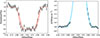 |
Fig. 1. Normalized radio light curve of PSR J1932+2121 during the eclipse period (left) and the corresponding DM variation (right). The solid lines give the fitting of the data with the model and 1σ confidence regions shown as shaded areas. The adopted parameter values are listed in Table 1. |
Parameters of PSR J1932+2121.
3. The radio eclipse
The periodic eclipse of pulsar radio emission can occur due to the orbital motion of the companion star around the pulsar when the LOS direction passes through the companion star and its outflows within an IBS shock (Du et al. 2023). Such an IBS, also known as a bow shock, can arise from the interaction between the relativistic pulsar wind and the companion wind (Bosch-Ramon & Khangulyan 2011; Romani & Sanchez 2016; Wadiasingh et al. 2017; Kandel et al. 2021). The geometry of this shock is determined by mechanical pressure balance across the contact discontinuity, and is primarily governed by the momentum flux ratio of the two winds as
 (2)
(2)
where Lsd is the spin-down power of the pulsar, c is the speed of light, ṀC is the mass-loss rate of the companion star, and vw is the terminal velocity of this wind. For constants ṀC and vw, the number density of the companion wind can be written as
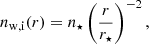 (3)
(3)
where the base density n★ at the stellar surface r★ is given by  with mp the mass of protons and r the distance from the center of the companion.
A detailed description of the radio eclipse mechanism for spider pulsars was provided by Thompson et al. (1994). It was further ruled out that the eclipse is caused by scattering and refraction (Broderick et al. 2016; Kudale et al. 2020); instead, the absorption process could play the most important role in suppressing the pulsar radio emission. Then, with a frequency-dependent absorption coefficient α(ν, ne), we can express the eclipse using the absorption optical depth along the LOS as (Chen et al. 2021a)
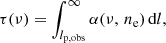 (4)
(4)
which strongly depends on the physical process dominating the absorption. Here, lp, obs is aimed at describing the shock cavity size, and ne is the electron number density, which is determined by the hydrogen abundance of the wind and the distance to the center of the companion star. Specifically, the electron number density can be related to the ion density by ne = nw, iμi/μe, where μi ∼ 1.29 and μe ∼ 1.18 are the typical values for the mean ion molecular weight and electron weight, respectively (Zdziarski et al. 2010). This optical depth determines the attenuation of the pulsar radio emission and is therefore constrained by the observed flux variations during the eclipse. Meanwhile, the enhanced electron density along the LOS can contribute an extra component of the dispersion measure (DM), which can be expressed as
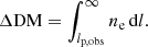 (5)
(5)
The observed variations of the radio flux and DM jointly constrain the location and path length of the LOS through the eclipsing medium enveloped by the bow shock, thereby effectively constraining the IBS geometry represented by lp, obs.
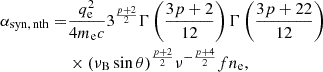
For the eclipse mechanism, measurements of magnetic fields in the eclipse medium indicated that the cyclotron–synchrotron absorption mechanism may play a more important role in radio absorption (Polzin et al. 2019; Lin et al. 2023; Wang et al. 2023). Specifically, the measured magnetic field strength could be too low to meet the requirement of cyclotron absorption (Thompson et al. 1994; Li et al. 2019; Kumari et al. 2024); furthermore, cyclotron absorption cannot account for the observed broadband as it is expected to feature at the cyclotron frequency and its harmonics (Khechinashvili et al. 2000; Kansabanik et al. 2021). Alternatively, some recent studies suggested that the eclipse could be dominated by synchrotron absorption, such as the 4 GHz eclipse of PSR J1908+2105 (Ghosh et al. 2025). Therefore, in this work we took into account synchrotron absorption with an absorption coefficient given by (Yang et al. 2016; Ghosh et al. 2025)
 (6)
(6)
where qe and me are the electron charge and mass, νB = qeBm/2πmec is the Larmor frequency of the electron, Bm is the local magnetic field strength, θ is the angle between the LOS and magnetic field lines, Γ denotes the Gamma function, and p is the power-law (PL) index of the nonthermal electron distribution. In the above expression, a PL distribution with index p is adopted as
 (7)
(7)
for relativistic nonthermal electrons in the medium, where γmin and γmax are the minimum and maximum Lorentz factors, respectively, and fnth represents the fraction of nonthermal electrons. In the following calculations, we took the combination coefficient f as a free parameter and assumed the PL index p to be 2.5 as a fiducial value for the nonthermal electron distribution. In comparison, the contribution of thermal electrons is ignored, which can be safe as long as the electron temperature satisfies kBTe ≲ 0.1mec2.
In Fig. 1 we present the fitting results for the normalized flux and DM variations of PSR J1932+2121 during the eclipse; the 1σ confidence regions are shown as shaded areas. The corresponding best-fit parameters are summarized in Table 2. The inferred orbital inclination is approximately  , indicating that the orbit of PSR J1932+2121 is viewed nearly edge-on. The mass-loss rate and the velocity of the companion wind are constrained to be 10−12.46 M⊙ yr−1 and 0.34 × 108 cm s−1, respectively. These parameter values are consistent with the companion being a low-mass main-sequence star (Wang et al. 2025). Meanwhile, with such a weak stellar wind and a pulsar spin-down luminosity of 4.81 × 1033 erg s−1, the evaporation efficiency is only ∼10−4, thus indicating that ablation of the companion is highly inefficient, which allows the system to remain in a relatively stable state for a long time (Misra et al. 2025).
Fitting parameters.
4. Pulsar wind dynamics and X-ray emission prospects
4.1. Implication for the dynamics of pulsar wind
Initially, the pulsar wind is dominated by the Poynting flux, and the conversion of electromagnetic energy into bulk kinetic energy during wind expansion reduces magnetization with increasing radius (Bogovalov 1999; Aharonian et al. 2012; Takata & Cheng 2017; Sullivan & Romani 2024). The evolution of particles in the pulsar wind can be derived from relativistic magnetohydrodynamics (MHD) by accounting for magnetic reconnection (MR) as the dominant dissipation mechanism (Lyubarsky & Kirk 2001; Drenkhahn & Spruit 2002; Cortés & Sironi 2024). In the following, we refer to this case as the MR model. Under the assumption that the magnetic energy is entirely converted into bulk kinetic energy rather than particle internal energy, the dynamical description can be obtained by numerically solving the equation as follows (Drenkhahn 2002):
![Mathematical equation: $$ \begin{aligned} \frac{\mathrm{d} \Gamma _{\mathrm{w} }}{\mathrm{d} l} = \frac{2}{c \, \tau } \left[ (1 - \mu ^2)(1 + \sigma _{\mathrm{LC} }) \Gamma _{\mathrm{LC} } + \mu ^2 \Gamma _{\mathrm{LC} } - \Gamma _{\mathrm{w} } \right] . \end{aligned} $$](/articles/aa/full_html/2026/07/aa59647-26/aa59647-26-eq16.gif) (8)
(8)
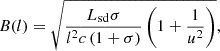
Here Γw is the bulk Lorentz factor of the pulsar wind; τ is the MR timescale; μ = cos i is the magnetic obliquity, with i the angle between the spin and magnetic axes of the pulsar; and σLC and ΓLC are the magnetization parameter and the Lorentz factor at light-cylinder radius rLC, respectively. Furthermore, the compression of the magnetic field at the shock can be derived by applying the MHD shock jump conditions with the magnetization in the pulsar wind (Kennel & Coroniti 1984; Chen et al. 2019),
 (9)
(9)
where u is the radial four velocity. Kandel et al. (2019) assumed a toroidal magnetic field structure in the pulsar wind outside the light cylinder as B(l) = B0(l0/l), where B0 = (3Lsd/2 c l02)1/2 is the magnetic field at the nose of the shock l0 (Kandel et al. 2019; Sullivan & Romani 2023). In the relativistic limit u ≫ 1 and for a slowly varying σ(l), Eq. (9) simplifies to B ∝ l−1, which exhibits the same radial decrease as the toroidal model. We found that the two magnetic field descriptions are broadly similar over most of the shock region, but their differences become more pronounced in the distant shock tail, as shown in the right panel of Fig. 2.
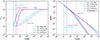 |
Fig. 2. Bulk Lorentz factor (left) and the magnetic field distribution (right) in pulsar wind with distance from the light-cylinder radius rLC for the MR and PL magnetization decay models with different spin period of Pspin = 2.5 ms and 14.25 ms. The dotted line indicates the position of the IBS nose, i.e., the shock stand-off distance (l0). In the left panel, the horizontal dotted line depicts the maximum Lorentz factor Γmax, corresponding to complete conversion of the available Poynting flux into bulk kinetic energy. In the right panel, the toroidal field model (B ∝ l−1) is compared with the MHD-compressed field derived from shock jump conditions. |
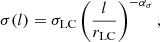
Meanwhile, some investigations suggest that MR in the striped pulsar wind is not a highly efficient method for converting Poynting energy into bulk kinetic energy, and the magnetization of the pulsar wind is assumed to evolve with radial distance in the form of a PL, which we hereafter refer to as the PL model (Kong et al. 2012; Takata & Cheng 2017),
 (10)
(10)
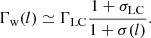
where ασ is taken to be 1.5. Correspondingly, according to energy conservation, the Lorentz factor and magnetization in the pulsar wind zone are related by (Chen et al. 2021b)
 (11)
(11)
Moreover, the faster dissipation of magnetic energy in the PL model results in a weaker magnetic field on the shock nose and decays more sharply with distance toward the shock tail.
The resulting Lorentz factor profiles for a spin period of 14.25 ms (PSR J1932+2121) and a typical MSP value of 2.5 ms, corresponding to the median spin period of spider pulsars (Koljonen & Linares 2025), are shown in the left panel of Fig. 2. The PL model indicates that the particles can be fully accelerated at the shock nose regardless of the spin period. In contrast, in MR dissipation, magnetic energy cannot be fully converted into bulk kinetic energy at the shock nose, leading to a lower Lorentz factor for the slower-spinning pulsar.
4.2. The emission of the IBS
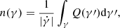
The pulsar wind is terminated by the stellar outflows, forming a contact discontinuity that separates two shocked regions. The pulsar wind carries and dissipates most of the Poynting flux energy and is highly magnetized and relativistic downstream of the shock, whereas the companion wind remains comparatively nonrelativistic and weakly magnetized (Wadiasingh et al. 2017; Cortés & Sironi 2024, 2025). Therefore, we focus on the IBS region where upstream electrons of the pulsar wind are accelerated to ultra-relativistic energies and subsequently cool through adiabatic or radiative processes (Lyubarsky 2003; Sironi & Spitkovsky 2011; Kandel et al. 2021; Sullivan & Romani 2025). The accelerated electron–positron pairs are assumed to be distributed as a PL, Q(γ) = Q0γ−p, where Q0 is the injection rate per unit volume and per unit γ. Under the steady-state assumption, the post-shock distribution of shocked electrons can be expressed by the solution of the continuity equation as (Zabalza et al. 2013; Chen et al. 2019)
 (12)
(12)
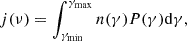
where  is the total energy loss rate. By accounting for synchrotron cooling, which dominates the energy losses of electrons traveling downstream in the shock magnetic field (Ghisellini 2013; Cortés & Sironi 2022, 2025), we can calculate the emissivity of the shock by
 (13)
(13)
where P(γ) is the synchrotron power of a single electron. The minimum Lorentz factor of the shocked electrons is determined by the pulsar wind at the pre-shock region, which is given by
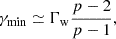 (14)
(14)
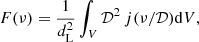
which is highly dependent on the bulk Lorentz factor of the injecting pulsar wind. The maximum Lorentz factor depends on the acceleration and cooling process, which can be obtained as γmax = (6πqe/σTB)1/2. The relativistic bulk motion of the shocked flow causes the emission from the downstream to be strongly beamed, resulting in a Doppler boost at the shock tail when the beaming direction passes through the LOS (Dubus et al. 2010; Wadiasingh et al. 2017; van der Merwe et al. 2020; Cortés & Sironi 2025). Thus, the total flux from the bow shock can be calculated as (Granot et al. 1999; Kandel et al. 2019)
 (15)
(15)
where 𝒟 is the Doppler factor determined by the bulk Lorentz factor and the angle between the flow direction and the LOS (Kathirgamaraju et al. 2018; Chen et al. 2021b).
4.3. X-ray spectra and light curves
We further investigated the high-energy synchrotron emission originating from the IBS by the emission model with a magnetization parameter of 102 at rLC and a particle distribution index of 2.1. Figure 3 shows the calculated spectral energy distribution (SED) of PSR J1932+2121 at the phase of shock flow along the LOS with strong Doppler boosting (Dubus et al. 2010; Kandel et al. 2019). Although our main interest here is the X-ray detectability of the IBS emission, the modeled SED naturally extends to higher energies, so the Fermi/LAT upper limit is also shown as an additional constraint on the high-energy tail of the spectrum. Since no optical counterpart has been detected, the distance is estimated to be 1.5 ∼ 5.1 kpc (Misra et al. 2025). Here we used the shaded region to depict the uncertainty of the distance, while the solid curve in Fig. 3 represents the calculation performed at the average distance of 3.3 kpc. For PSR J1932+2121 with Pspin = 14.25 ms, the predicted X-ray SED lies close to or below the current sensitivity limits when the pulsar wind magnetic energy dissipation is governed by the MR model. In contrast, if the Poynting flux is dissipated according to the PL model of σ(l), the resulting IBS emission becomes significantly brighter and can exceed the typical X-ray SED expected for MSPs. Therefore, future deep X-ray observations of PSR J1932+2121 will provide a useful test of the pulsar wind Poynting energy dissipation and can place meaningful constraints on the wind dynamics. Moreover, the integrated X-ray flux in the 0.5−12 keV band from the IBS region is shown in Fig. 4. The double-peaked flux profile over one orbital period arises from Doppler boosting of the shocked flow, which is modeled with a Lorentz factor of 1.8, as the LOS passes across the bow shock twice around the eclipse (Sim et al. 2024). It is conceivable that when the orbital inclination is small or the half-opening angle of the shock is narrow, the double-peak structure may merge into a single peak (An et al. 2018; Park et al. 2025).
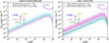 |
Fig. 3. SED of PSR J1932+2121 at the phase of shock flow along the LOS, shown for the MR (left) and PL magnetization decay (right) models. The shaded region indicates the uncertainty associated with the source distance, taken to be 1.5 ∼5.1 kpc by Misra et al. (2025), while the solid line running through the middle of each shaded region corresponds to the calculation with the adopted average distance of 3.3 kpc. The sensitivity limits for Swift, EP/FXT, XMM/EPIC, and eXTP/SFA are adopted from Burrows et al. (2005), Yuan et al. (2022), Traulsen et al. (2019), and Zhang et al. (2019), respectively, assuming representative exposure times of 1–100 ks. The upper limits of Fermi/LAT are from Werner et al. (2013) and are shown as an additional constraint on the high-energy tail of the spectrum. |
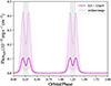 |
Fig. 4. Predicted 0.5−12 keV X-ray light curve from the IBS region of PSR J1932+2121. The gray band represents the orbital phase range of the eclipse, and the purple shaded region indicates the flux uncertainty due to the distance range estimated by Misra et al. (2025). The central solid curve corresponds to the calculation with the adopted average distance of 3.3 kpc. |
5. Summary
The newly discovered redback pulsar binary system with radio eclipse of PSR J1932+2121 by FAST provides an opportunity to constrain the binary orbit and the properties of the companion and pulsar. Based on fitting the orbital-phase-dependent DM variations by the eclipse model, we inferred a nearly edge-on inclination of  and a weak companion stellar wind of ṀC ∼ 10−12.46 M⊙ yr−1 with vw ∼ 0.34 × 108cm s−1, consistent with a low-mass main-sequence star.
We further modeled the high-energy emission from the IBS zone by explicitly incorporating pulsar wind dynamics, in which MR progressively reduces wind magnetization, and MHD compression at the shock produces a magnetic field scaling similar to the toroidal field assumed by Kandel et al. (2019). The resulting shock synchrotron emission predicts a detectable X-ray flux near the INFC phase with XMM/EPIC, EP/FXT, or eXTP/SFA, while the γ-ray flux remains below current Fermi/LAT limits. At present, there is no cataloged Fermi/LAT source positionally coincident with PSR J1932+2121, which is qualitatively consistent with this result. Taking into account the distance uncertainty, the phase-resolved 0.5−12 keV light curve exhibits a characteristic double-peaked light curve around the eclipse range, shaped by Doppler boosting in the post-shock flow. These high-energy radiation features of PSR J1932+2121 can be tested in future observations. Furthermore, the long spin period of the pulsar (Pspin = 14.25 ms) and weak companion stellar wind suggest only mild recycling and inefficient late-stage accretion. This implies that the actual mass of this neutron star is likely slightly greater than the canonical 1.4 M⊙ typically assumed (Özel & Freire 2016), while still far from the extreme ≳2 M⊙ regime.
Acknowledgments
We are grateful to Bing-Qing Zhou for helpful discussions and suggestions. This work is supported by the National Natural Science Foundation of China (grant Nos. 12393811, 12303047 and 12588202), the National SKA Program of China (2020SKA0120300), and the National Key R&D Program of China (Nos. 2021YFA0718500 and 2025YFA161400).
References
- Aharonian, F. A., Bogovalov, S. V., & Khangulyan, D. 2012, Nature, 482, 507 [NASA ADS] [CrossRef] [Google Scholar]
- An, H., Romani, R. W., & Kerr, M. 2018, ApJ, 868, L8 [Google Scholar]
- Bilous, A. V., Ransom, S. M., & Demorest, P. 2019, ApJ, 877, 125 [Google Scholar]
- Bogovalov, S. V. 1999, A&A, 349, 1017 [Google Scholar]
- Bosch-Ramon, V., & Khangulyan, D. 2011, PASJ, 63, 1023 [NASA ADS] [Google Scholar]
- Broderick, J. W., Fender, R. P., Breton, R. P., et al. 2016, MNRAS, 459, 2681 [Google Scholar]
- Burrows, D. N., Hill, J. E., Nousek, J. A., et al. 2005, Space Sci. Rev., 120, 165 [Google Scholar]
- Chen, H.-L., Chen, X., Tauris, T. M., & Han, Z. 2013, ApJ, 775, 27 [NASA ADS] [CrossRef] [Google Scholar]
- Chen, A. M., Takata, J., Yi, S. X., Yu, Y. W., & Cheng, K. S. 2019, A&A, 627, A87 [NASA ADS] [CrossRef] [EDP Sciences] [Google Scholar]
- Chen, A. M., Guo, Y. D., Yu, Y. W., & Takata, J. 2021a, A&A, 652, A39 [NASA ADS] [CrossRef] [EDP Sciences] [Google Scholar]
- Chen, A.-M., Ng, C., Takata, J., & Yu, Y.-W. 2021b, RAA, 21, 189 [Google Scholar]
- Cortés, J., & Sironi, L. 2022, ApJ, 933, 140 [CrossRef] [Google Scholar]
- Cortés, J., & Sironi, L. 2024, MNRAS, 534, 2551 [Google Scholar]
- Cortés, J., & Sironi, L. 2025, MNRAS, 542, 917 [Google Scholar]
- de Martino, D., Papitto, A., Burgay, M., et al. 2020, MNRAS, 492, 5607 [Google Scholar]
- Drenkhahn, G. 2002, A&A, 387, 714 [NASA ADS] [CrossRef] [EDP Sciences] [Google Scholar]
- Drenkhahn, G., & Spruit, H. C. 2002, A&A, 391, 1141 [NASA ADS] [CrossRef] [EDP Sciences] [Google Scholar]
- Du, Z.-X., Yu, Y.-W., Chen, A. M., et al. 2023, RAA, 23, 125024 [Google Scholar]
- Dubus, G., Cerutti, B., & Henri, G. 2010, A&A, 516, A18 [NASA ADS] [CrossRef] [EDP Sciences] [Google Scholar]
- Fruchter, A. S., Gunn, J. E., Lauer, T. R., & Dressler, A. 1988, Nature, 334, 686 [Google Scholar]
- Ghisellini, G. 2013, Radiative Processes in High Energy Astrophysics, 873 [Google Scholar]
- Ghosh, A., Bhattacharyya, B., Kumari, S., et al. 2025, ApJ, 982, 168 [Google Scholar]
- Granot, J., Piran, T., & Sari, R. 1999, ApJ, 513, 679 [NASA ADS] [CrossRef] [Google Scholar]
- Guillemot, L., Octau, F., Cognard, I., et al. 2019, A&A, 629, A92 [NASA ADS] [CrossRef] [EDP Sciences] [Google Scholar]
- Han, J. L., Wang, C., Wang, P. F., et al. 2021, RAA, 21, 107 [Google Scholar]
- Han, J. L., Zhou, D. J., Wang, C., et al. 2025, RAA, 25, 014001 [Google Scholar]
- Hobbs, G. B., Edwards, R. T., & Manchester, R. N. 2006, MNRAS, 369, 655 [Google Scholar]
- Hotan, A. W., van Straten, W., & Manchester, R. N. 2004, PASA, 21, 302 [Google Scholar]
- Huang, H. H., & Becker, W. 2007, A&A, 463, L5 [NASA ADS] [CrossRef] [EDP Sciences] [Google Scholar]
- Kandel, D., Romani, R. W., & An, H. 2019, ApJ, 879, 73 [NASA ADS] [CrossRef] [Google Scholar]
- Kandel, D., Romani, R. W., & An, H. 2021, ApJ, 917, L13 [NASA ADS] [CrossRef] [Google Scholar]
- Kansabanik, D., Bhattacharyya, B., Roy, J., & Stappers, B. 2021, ApJ, 920, 58 [NASA ADS] [CrossRef] [Google Scholar]
- Karpova, A. V., Zharikov, S. V., Zyuzin, D. A., et al. 2025, A&A, 693, A158 [NASA ADS] [CrossRef] [EDP Sciences] [Google Scholar]
- Kathirgamaraju, A., Barniol Duran, R., & Giannios, D. 2018, MNRAS, 473, L121 [Google Scholar]
- Kennel, C. F., & Coroniti, F. V. 1984, ApJ, 283, 710 [Google Scholar]
- Khechinashvili, D. G., Melikidze, G. I., & Gil, J. A. 2000, ApJ, 541, 335 [Google Scholar]
- Kluzniak, W., Ruderman, M., Shaham, J., & Tavani, M. 1988, Nature, 334, 225 [NASA ADS] [CrossRef] [Google Scholar]
- Koljonen, K. I. I., & Linares, M. 2025, ApJ, 994, 8 [Google Scholar]
- Kong, S. W., Cheng, K. S., & Huang, Y. F. 2012, ApJ, 753, 127 [NASA ADS] [CrossRef] [Google Scholar]
- Kudale, S., Roy, J., Bhattacharyya, B., Stappers, B., & Chengalur, J. 2020, ApJ, 900, 194 [Google Scholar]
- Kumari, S., Bhattacharyya, B., Sharan, R., et al. 2024, ApJ, 973, 19 [Google Scholar]
- Kumari, S., Bhattacharyya, B., Kansabanik, D., et al. 2025, ApJ, 979, 143 [Google Scholar]
- Li, D., Lin, F. X., Main, R., et al. 2019, MNRAS, 484, 5723 [NASA ADS] [CrossRef] [Google Scholar]
- Lin, F. X., Main, R. A., Jow, D., et al. 2023, MNRAS, 519, 121 [Google Scholar]
- Lyubarsky, Y. E. 2003, MNRAS, 345, 153 [Google Scholar]
- Lyubarsky, Y., & Kirk, J. G. 2001, ApJ, 547, 437 [NASA ADS] [CrossRef] [Google Scholar]
- Miao, C.-C., Blackmon, V., Zhu, W.-W., et al. 2023, RAA, 23, 105005 [Google Scholar]
- Misra, D., Koljonen, K. I. I., & Linares, M. 2025, MNRAS, 541, L58 [Google Scholar]
- Nieder, L., Clark, C. J., Kandel, D., et al. 2020, ApJ, 902, L46 [NASA ADS] [CrossRef] [Google Scholar]
- Özel, F., & Freire, P. 2016, ARA&A, 54, 401 [Google Scholar]
- Pan, Z., Ransom, S. M., Lorimer, D. R., et al. 2020, ApJ, 892, L6 [NASA ADS] [CrossRef] [Google Scholar]
- Park, J., Kim, C., An, H., & Wadiasingh, Z. 2025, Astron. Nachr., 346, e20240099 [Google Scholar]
- Phinney, E. S. 1988, Bull. Am. Astron. Soc., 20, 981 [Google Scholar]
- Polzin, E. J., Breton, R. P., Stappers, B. W., et al. 2019, MNRAS, 490, 889 [Google Scholar]
- Polzin, E. J., Breton, R. P., Bhattacharyya, B., et al. 2020, MNRAS, 494, 2948 [Google Scholar]
- Roberts, M. S. E. 2013, Neutron Stars and Pulsars: Challenges and Opportunities after 80 years, 291, 127 [Google Scholar]
- Roberts, M. S. E., Mclaughlin, M. A., Gentile, P., et al. 2014, Astron. Nachr., 335, 313 [Google Scholar]
- Romani, R. W., & Sanchez, N. 2016, ApJ, 828, 7 [Google Scholar]
- Ruderman, M., Shaham, J., & Tavani, M. 1989, ApJ, 336, 507 [NASA ADS] [CrossRef] [Google Scholar]
- Satybaldiev, M., Linares, M., & Vecchiotti, V. 2026, ApJ, 998, 94 [Google Scholar]
- Sim, M., An, H., & Wadiasingh, Z. 2024, ApJ, 964, 109 [NASA ADS] [CrossRef] [Google Scholar]
- Sironi, L., & Spitkovsky, A. 2011, ApJ, 741, 39 [Google Scholar]
- Stappers, B. W. 1996, ASP Conf. Ser., 105, 517 [Google Scholar]
- Sullivan, A. G., & Romani, R. W. 2023, ApJ, 959, 81 [Google Scholar]
- Sullivan, A. G., & Romani, R. W. 2024, ApJ, 974, 315 [NASA ADS] [Google Scholar]
- Sullivan, A. G., & Romani, R. W. 2025, ApJ, 984, 146 [Google Scholar]
- Takata, J., & Cheng, K. S. 2017, ApJ, 834, 4 [NASA ADS] [CrossRef] [Google Scholar]
- Thompson, C., Blandford, R. D., Evans, C. R., & Phinney, E. S. 1994, ApJ, 422, 304 [Google Scholar]
- Traulsen, I., Schwope, A. D., Lamer, G., et al. 2019, A&A, 624, A77 [NASA ADS] [CrossRef] [EDP Sciences] [Google Scholar]
- van der Merwe, C. J. T., Wadiasingh, Z., Venter, C., Harding, A. K., & Baring, M. G. 2020, ApJ, 904, 91 [Google Scholar]
- Wadiasingh, Z., Harding, A. K., Venter, C., Böttcher, M., & Baring, M. G. 2017, ApJ, 839, 80 [NASA ADS] [CrossRef] [Google Scholar]
- Wang, S. Q., Wang, J. B., Li, D. Z., et al. 2023, ApJ, 955, 36 [Google Scholar]
- Wang, P. F., Han, J. L., Yang, Z. L., et al. 2025, RAA, 25, 014003 [Google Scholar]
- Werner, M., Reimer, O., Reimer, A., & Egberts, K. 2013, A&A, 555, A102 [NASA ADS] [CrossRef] [EDP Sciences] [Google Scholar]
- Yang, Y.-P., Zhang, B., & Dai, Z.-G. 2016, ApJ, 819, L12 [NASA ADS] [CrossRef] [Google Scholar]
- Yuan, W., Zhang, C., Chen, Y., & Ling, Z. 2022, in Handbook of X-ray and Gamma-ray Astrophysics, eds. C. Bambi, & A. Sangangelo, 86 [Google Scholar]
- Zabalza, V., Bosch-Ramon, V., Aharonian, F., & Khangulyan, D. 2013, A&A, 551, A17 [NASA ADS] [CrossRef] [EDP Sciences] [Google Scholar]
- Zdziarski, A. A., Neronov, A., & Chernyakova, M. 2010, MNRAS, 403, 1873 [Google Scholar]
- Zhang, S., Santangelo, A., Feroci, M., et al. 2019, Sci. China Phys. Mech. Astron., 62, 29502 [Google Scholar]
Primary eclipses of pulsar emission are generally expected to occur in the orbital-phase interval near the INFC of the companion, during which the radio flux is strongly suppressed, accompanied by a synchronous DM excess. However, it is still noteworthy that some spider systems could exhibit irregular or weaker eclipse-like features in multiple orbital phases (e.g., PSR B1744-24A, PSR J1717+4308A, PSR J1810-1744; Bilous et al. 2019; Pan et al. 2020; Kumari et al. 2025), which might arise from clumps or otherwise complex material in the binary environment. Such complexity has not been discovered in PSR J1932+2121.
All Tables
All Figures
|
Fig. 1. Normalized radio light curve of PSR J1932+2121 during the eclipse period (left) and the corresponding DM variation (right). The solid lines give the fitting of the data with the model and 1σ confidence regions shown as shaded areas. The adopted parameter values are listed in Table 1. |
| In the text | |
|
Fig. 2. Bulk Lorentz factor (left) and the magnetic field distribution (right) in pulsar wind with distance from the light-cylinder radius rLC for the MR and PL magnetization decay models with different spin period of Pspin = 2.5 ms and 14.25 ms. The dotted line indicates the position of the IBS nose, i.e., the shock stand-off distance (l0). In the left panel, the horizontal dotted line depicts the maximum Lorentz factor Γmax, corresponding to complete conversion of the available Poynting flux into bulk kinetic energy. In the right panel, the toroidal field model (B ∝ l−1) is compared with the MHD-compressed field derived from shock jump conditions. |
| In the text | |
|
Fig. 3. SED of PSR J1932+2121 at the phase of shock flow along the LOS, shown for the MR (left) and PL magnetization decay (right) models. The shaded region indicates the uncertainty associated with the source distance, taken to be 1.5 ∼5.1 kpc by Misra et al. (2025), while the solid line running through the middle of each shaded region corresponds to the calculation with the adopted average distance of 3.3 kpc. The sensitivity limits for Swift, EP/FXT, XMM/EPIC, and eXTP/SFA are adopted from Burrows et al. (2005), Yuan et al. (2022), Traulsen et al. (2019), and Zhang et al. (2019), respectively, assuming representative exposure times of 1–100 ks. The upper limits of Fermi/LAT are from Werner et al. (2013) and are shown as an additional constraint on the high-energy tail of the spectrum. |
| In the text | |
|
Fig. 4. Predicted 0.5−12 keV X-ray light curve from the IBS region of PSR J1932+2121. The gray band represents the orbital phase range of the eclipse, and the purple shaded region indicates the flux uncertainty due to the distance range estimated by Misra et al. (2025). The central solid curve corresponds to the calculation with the adopted average distance of 3.3 kpc. |
| In the text | |
Current usage metrics show cumulative count of Article Views (full-text article views including HTML views, PDF and ePub downloads, according to the available data) and Abstracts Views on Vision4Press platform.
Data correspond to usage on the plateform after 2015. The current usage metrics is available 48-96 hours after online publication and is updated daily on week days.
Initial download of the metrics may take a while.