


| Issue |
A&A
Volume 709, May 2026
|
|
|---|---|---|
| Article Number | A252 | |
| Number of page(s) | 12 | |
| Section | Planets, planetary systems, and small bodies | |
| DOI | https://doi.org/10.1051/0004-6361/202659457 | |
| Published online | 22 May 2026 | |
Streaming instabilities in weakly ionized protoplanetary discs: The ambipolar streaming instability
1
Laboratoire d’astrophysique de Bordeaux, Univ. Bordeaux, CNRS, B18N, allée Geoffroy Saint-Hilaire,
33615
Pessac,
France
2
Institute of Astronomy and Astrophysics, Academia Sinica,
Taipei
10617,
Taiwan
3
Physics Division, National Center for Theoretical Sciences,
Taipei City
10617,
Taiwan
★ Corresponding author: This email address is being protected from spambots. You need JavaScript enabled to view it.
Received:
15
February
2026
Accepted:
10
April
2026
Abstract
The regions of protoplanetary disks in which planets can form are thought to be weakly ionized, which suggests that nonideal magnetohydrodynamics (MHD) effects play an important role in the disk dynamics and in the planet formation process. In particular, the combined effect of ohmic resistivity and ambipolar diffusion might cause the launch of MHD-driven disk winds. In this context, we focus on the effect of ambipolar diffusion (AD) and examine the stability of a dusty, magnetized disk by employing linear stability analyses and numerical simulations. We show that dust feedback tends to stabilize the MRI oblique modes of the magnetorotational instability (MRI) involved in the ambipolar shear instability. We also find that ambipolar diffusion leads to the onset of a strong resonant drag instability, in which an Alfvén wave is destabilized by the relative drift between the gas and dust components. The main effect of AD is to modify the Alfvén wave frequency, resulting in a large resonance width. The instability is found to have significant growth rates even in dust-poor discs and for tightly coupled particles, which may help to bridge the gap between the growth of dust grains through coagulation and planetesimal formation.
Key words: instabilities / methods: analytical / methods: numerical / planets and satellites: formation / protoplanetary disks
© The Authors 2026
 Open Access article, published by EDP Sciences, under the terms of the Creative Commons Attribution License (https://creativecommons.org/licenses/by/4.0), which permits unrestricted use, distribution, and reproduction in any medium, provided the original work is properly cited.
This article is published in open access under the Subscribe to Open model. This email address is being protected from spambots. You need JavaScript enabled to view it. to support open access publication.
1 Introduction
The first stage of planet formation involves the coagulation of micron-sized grains into millimeter-sized dust (Dullemond & Dominik 2005). However, the bouncing (Zsom et al. 2010) and fragmentation (Blum & Wurm 2008) barriers tend to prevent the further growth of solids, such that the way in which particles grow beyond the millimeter-size range remains an unanswered question. The streaming instability (hereafter SI, Youdin & Goodman 2005; Youdin & Johansen 2007), which arises from angular momentum exchange between the gas and dust components, has emerged as a leading mechanism to overcome these barriers. It has indeed been shown that gravitationally bound 100–1000 km sized bodies can form directly through the gravitational collapse of the filaments produced during the nonlinear evolution of the SI (Johansen et al. 2009; Simon et al. 2016; Abod et al. 2019). The original linear stability analysis, restricted to inviscid discs, indicates that the growth rate of the SI is highest for solids that are marginally coupled to the gas and for local dust-to-gas ratios ϵ higher than unity.
Recent works have extended this original linear analysis of the instability to examine whether the SI remains robust in the presence of external turbulence in the disk (Chen & Lin 2020; Umurhan et al. 2020). In the particular case when turbulence is driven by the magneto-rotational instability (hereafter MRI, Balbus & Hawley 1991), Johansen et al. (2007) found that the SI can still operate and lead to the formation of structures that concentrate into high-density regions; while Balsara et al. (2009) and Tilley et al. (2010) also reported significant dust clumping through the SI during the dust-settling process. However, except in its innermost regions, where thermal ionization guarantees that MRI operates, the bulk of the disk is expected to remain laminar because the ionization level of the gas is low. In these regions, nonideal MHD effects play an important role in the disk dynamics, as they can drive magnetically driven disk winds, which are thought to be the dominant mechanism for angular momentum transport in these discs (Bai & Stone 2013; Gressel et al. 2015; Béthune et al. 2017).
For these nonideal effects on the SI, Yang et al. (2018) considered a disk model that was sandwiched between a turbulent surface layer and a dead zone dominated by ohmic resistivity. The authors found that strong clumping of solids can arise in the dead zone due to a weak radial diffusion of particles near the midplane. On the other hand, by examining the stability of a dusty magnetized gas, Lin & Hsu (2022) found that in resistive discs, the SI can be stabilized by magnetic perturbations for low values of the dust-to-gas ratio. The consequence of the Hall effect on the SI was investigated by Wu et al. (2024). By employing a combination of linear analysis and numerical simulations, these authors found a new instability resulting from the advection of magnetic perturbations relative to the dusty gas, which can dominate the SI for low dust-to-gas ratios and weak magnetic fields.
We focus on the effect of ambipolar diffusion on the SI. Given the importance of ambipolar diffusion in the context of wind-driven protoplanetary discs, this is an important issue to consider. We find evidence for a strong resonant drag instability (hereafter RDI; Squire & Hopkins 2018a,b; Zhuravlev 2019) resulting from the destabilization of an ambipolar-modified Alfv’en wave by the relative drift between the gas and dust components. Compared to a standard Alfvén wave RDI (Hopkins & Squire 2018; Lin & Hsu 2022), ambipolar diffusion can trigger RDI over a wider range of wavelengths because it can modify the Alfvén frequency. We also find that dust can stabilize the unstable oblique modes of the MRI (Kunz & Balbus 2004; Desch 2004), giving rise to the ambipolar-shear instability.
The paper is organized as follows. In Sect. 2 we present the governing evolution equations of the gas and dust components. We then describe in Sect. 3 the linear theory and present numerical solutions to the linear stability problem in Sect. 4. In Sect. 5, we discuss the effect of ambipolar diffusion on the Alfvén wave RDI. In Sect. 6 we present the results of nonlinear simulations of the instability. We finally summarize our findings in Sect. 7.
2 Physical model
2.1 Shearing sheet approximation
We modeled a local patch in a protoplanetary disk within the shearing-box framework (Goldreich & Lynden-Bell 1965; Latter & Papaloizou 2017). A Cartesian coordinate system with the origin located at an arbitrary distance R0 from the central star corotates with angular velocity Ω = Ωk(R0), with Ωk the Keplerian angular velocity. The x- and y-axes were oriented radially outward and along the orbital direction, respectively, while the z-axis was directed in the vertical direction. We assumed that the domain is small compared to the orbital distance so that Keplerian rotation appears as a linear shear flow with velocity ![Mathematical equation: $\[\mathbf{U}_{\mathbf{k}}=-\frac{3}{2} x \Omega \hat{\mathbf{y}}\]$](/articles/aa/full_html/2026/05/aa59457-26/aa59457-26-eq1.png) . We assumed that the system is axisymmetric and neglected the vertical component of stellar gravity. In these limits, the continuity and momentum equations for the gas and dust components are given by
. We assumed that the system is axisymmetric and neglected the vertical component of stellar gravity. In these limits, the continuity and momentum equations for the gas and dust components are given by
![Mathematical equation: $\[\frac{\partial \rho_g}{\partial t}+\nabla \cdot\left(\rho_g \mathbf{v}\right)=0\]$](/articles/aa/full_html/2026/05/aa59457-26/aa59457-26-eq2.png) (1)
(1)
![Mathematical equation: $\[\begin{aligned}\frac{\partial \mathbf{v}}{\partial t}+\mathbf{v} \cdot \nabla \mathbf{v}-2 v_y \Omega \hat{\mathbf{x}}+v_x \frac{\Omega}{2} \hat{\mathbf{y}}= & 2 \eta R \Omega^2 \hat{\mathbf{x}}-\frac{1}{\rho_g} \nabla\left(P+\frac{B^2}{2 \mu_0}\right) \\& +\frac{1}{\rho_g \mu_0}(\mathbf{B} \cdot \nabla) \mathbf{B}+\frac{\epsilon}{\tau_s}(\mathbf{w}-\mathbf{v})\end{aligned}\]$](/articles/aa/full_html/2026/05/aa59457-26/aa59457-26-eq3.png) (2)
(2)
![Mathematical equation: $\[\frac{\partial \rho_d}{\partial t}+\nabla \cdot\left(\rho_d \mathbf{w}\right)=0\]$](/articles/aa/full_html/2026/05/aa59457-26/aa59457-26-eq4.png) (3)
(3)
![Mathematical equation: $\[\frac{\partial \mathbf{w}}{\partial t}+\mathbf{w} \cdot \nabla \mathbf{w}-2 w_y \Omega \hat{\mathbf{x}}+w_x \frac{\Omega}{2} \hat{\mathbf{y}}=-\frac{1}{\tau_s}(\mathbf{w}-\mathbf{v}),\]$](/articles/aa/full_html/2026/05/aa59457-26/aa59457-26-eq5.png) (4)
(4)
respectively, where ρg and ρd are the gas and dust densities, respectively, v and w are their velocities measured relatively to the background Keplerian shear, and μ0 is the magnetic permeability. We adopted an isothermal equation of state with the pressure given by ![Mathematical equation: $\[P=\rho_{g} c_{s}^{2}\]$](/articles/aa/full_html/2026/05/aa59457-26/aa59457-26-eq6.png) , where cs = HgΩ is the (constant) sound speed, with Hg the gas-pressure scale height. In Eq. (2), the term ∝ η corresponds to an outward force acting on the gas through a background radial pressure gradient and is determined by the dimensionless parameter
, where cs = HgΩ is the (constant) sound speed, with Hg the gas-pressure scale height. In Eq. (2), the term ∝ η corresponds to an outward force acting on the gas through a background radial pressure gradient and is determined by the dimensionless parameter
![Mathematical equation: $\[\eta=-\frac{1}{2 \rho_g \Omega^2 R_0} \frac{\partial P}{\partial r}.\]$](/articles/aa/full_html/2026/05/aa59457-26/aa59457-26-eq7.png) (5)
(5)
Finally, ϵ = ρd/ρg is the dust-to-gas ratio, and τs is the stopping time that we characterized in the following in terms of the dimensionless Stokes number: St = τsΩ.
The induction equation is given by
![Mathematical equation: $\[\frac{\partial \mathbf{B}}{\partial t}=\nabla \times(\mathbf{v} \times \mathbf{B})-\frac{3}{2} \Omega B_x \hat{\mathbf{y}}+\nabla \times\left[\frac{1}{\gamma_{i n} \rho_i \rho_g}(\mathbf{J} \times \mathbf{B}) \times \mathbf{B}\right],\]$](/articles/aa/full_html/2026/05/aa59457-26/aa59457-26-eq8.png) (6)
(6)
where ![Mathematical equation: $\[\mathbf{J} \equiv \mu_{0}^{-1} \nabla \times \mathbf{B}\]$](/articles/aa/full_html/2026/05/aa59457-26/aa59457-26-eq9.png) is the current density, γin is the ion-neutral drag coefficient, and ρi is the ion mass density.
is the current density, γin is the ion-neutral drag coefficient, and ρi is the ion mass density.
2.2 Equilibrium state
In the following, we assumed a constant magnetic field and null radial component. In practice, any radial component is sheared by differential rotation such that the radial component rapidly becomes much smaller that the azimuthal component. Under these conditions, there is no deviation from Keplerian rotation because the magnefic field and the equilibrium conditions correspond to the traditional steady-state drift solutions for a dusty disk obtained by Nakagawa et al. (1986). For constant values of ρg, ρd, and St, equilibrium solutions to Eqs. (1)–(4) can be obtained, leading to velocity deviations from Keplerian rotation given by
![Mathematical equation: $\[v_x=\frac{2 \epsilon \mathrm{St}}{\Delta^2} \eta R_0 \Omega,\]$](/articles/aa/full_html/2026/05/aa59457-26/aa59457-26-eq10.png) (7)
(7)
![Mathematical equation: $\[v_y=-\frac{\left(1+\epsilon+\mathrm{St}^2\right)}{\Delta^2} \eta R_0 \Omega,\]$](/articles/aa/full_html/2026/05/aa59457-26/aa59457-26-eq11.png) (8)
(8)
![Mathematical equation: $\[w_x=\frac{-2 \mathrm{St}}{\Delta^2} \eta R_0 \Omega,\]$](/articles/aa/full_html/2026/05/aa59457-26/aa59457-26-eq12.png) (9)
(9)
![Mathematical equation: $\[w_y=-\frac{(1+\epsilon)}{\Delta^2} \eta R_0 \Omega,\]$](/articles/aa/full_html/2026/05/aa59457-26/aa59457-26-eq13.png) (10)
(10)
where Δ2 = St2 + (1 + ϵ)2.
3 Linear theory
3.1 Linearized equations
In this section, we perturb Eqs. (1)–(6) assuming a background field ![Mathematical equation: $\[\mathbf{B}=B_{y} \hat{\mathbf{y}}+B_{z} \hat{\mathbf{z}}\]$](/articles/aa/full_html/2026/05/aa59457-26/aa59457-26-eq14.png) , with By (Bz) the azimuthal (vertical) component of the magnetic field. For any variable A, we also assumed Eulerian perturbations such that
, with By (Bz) the azimuthal (vertical) component of the magnetic field. For any variable A, we also assumed Eulerian perturbations such that
![Mathematical equation: $\[\left.A \rightarrow A+\delta A ~\exp \left[i\left(k_x x+k_z z\right)+\sigma t\right)\right],\]$](/articles/aa/full_html/2026/05/aa59457-26/aa59457-26-eq15.png) (11)
(11)
where linearized quantities are indicated by the δ notation, and where kx (kz) is the radial (vertical) wavenumber. Under these conditions, the linearized equations for our dusty magnetized disk are given by
![Mathematical equation: $\[\sigma W=-i\left(k_x \delta v_x+k_z \delta v_z\right)-i k_x v_x W\]$](/articles/aa/full_html/2026/05/aa59457-26/aa59457-26-eq16.png) (12)
(12)
![Mathematical equation: $\[\begin{aligned}\sigma \delta v_x= & 2 \Omega \delta v_y-i k_x v_x \delta v_x-\frac{\epsilon}{\tau_s}\left(v_x-w_x\right)(Q-W)-\frac{\epsilon}{\tau_s}\left(\delta v_x-\delta w_x\right) \\& -i k_x c_s^2 W+i c_{A, z}^2\left(k_z \delta b_x-k_x \delta b_z-k_x B_y^{\prime} \delta b_y\right)\end{aligned}\]$](/articles/aa/full_html/2026/05/aa59457-26/aa59457-26-eq17.png) (13)
(13)
![Mathematical equation: $\[\begin{aligned}\sigma \delta v_y= & -\frac{\Omega}{2} \delta v_x-i k_x v_x \delta v_y-\frac{\epsilon}{\tau_s}\left(v_y-w_y\right)(Q-W) \\& -\frac{\epsilon}{\tau_s}\left(\delta v_y-\delta w_y\right)+i c_{A, z}^2 k_z \delta b_y\end{aligned}\]$](/articles/aa/full_html/2026/05/aa59457-26/aa59457-26-eq18.png) (14)
(14)
![Mathematical equation: $\[\sigma \delta v_z=-i k_x v_x \delta v_z-\frac{\epsilon}{\tau_s}\left(\delta v_z-\delta w_z\right)-i k_z c_s^2 W-i c_{A, z}^2 k_z B_y^{\prime} \delta b_y\]$](/articles/aa/full_html/2026/05/aa59457-26/aa59457-26-eq19.png) (15)
(15)
![Mathematical equation: $\[\sigma Q=-i\left(k_x \delta w_x+k_z \delta w_z\right)-i k_x w_x Q\]$](/articles/aa/full_html/2026/05/aa59457-26/aa59457-26-eq20.png) (16)
(16)
![Mathematical equation: $\[\sigma \delta w_x=2 \Omega \delta w_y-i k_x w_x \delta w_x-\frac{1}{\tau_s}\left(\delta w_x-\delta v_x\right)\]$](/articles/aa/full_html/2026/05/aa59457-26/aa59457-26-eq21.png) (17)
(17)
![Mathematical equation: $\[\sigma \delta w_y=-\frac{\Omega}{2} \delta w_x-i k_x w_x \delta w_y-\frac{1}{\tau_s}\left(\delta w_y-\delta v_y\right)\]$](/articles/aa/full_html/2026/05/aa59457-26/aa59457-26-eq22.png) (18)
(18)
![Mathematical equation: $\[\sigma \delta w_z=-i k_x w_x \delta w_z-\frac{1}{\tau_s}\left(\delta w_z-\delta v_z\right)\]$](/articles/aa/full_html/2026/05/aa59457-26/aa59457-26-eq23.png) (19)
(19)
![Mathematical equation: $\[\sigma \delta b_x=i k_z \delta v_x-i k_x v_x \delta b_x+\eta_{\mathrm{AD}}(-k^2 \delta b_x+k_x k_z B_y^{\prime} \delta b_y)\]$](/articles/aa/full_html/2026/05/aa59457-26/aa59457-26-eq24.png) (20)
(20)
![Mathematical equation: $\[\begin{aligned}\sigma \delta b_y= & i k_z \delta v_y-i\left(k_x \delta v_x+k_z \delta v_z\right) B_y^{\prime}-i k_x v_x \delta b_y-\frac{3}{2} \Omega \delta b_x \\& +\eta_{\mathrm{AD}}\left[k^2 \frac{k_x}{k_z} B_y^{\prime} \delta b_x-\left(k^2 B_y^{\prime 2}+k_z^2\right) \delta b_y\right]\end{aligned}\]$](/articles/aa/full_html/2026/05/aa59457-26/aa59457-26-eq25.png) (21)
(21)
![Mathematical equation: $\[\begin{aligned}\sigma \delta b_z= & -i k_x \delta v_x-i k_x v_x \delta b_z \\& +\eta_{\mathrm{AD}}(k_x k_z \delta b_x-k_x^2 B_y^{\prime} \delta b_y-k_x^2 \delta b_z),\end{aligned}\]$](/articles/aa/full_html/2026/05/aa59457-26/aa59457-26-eq26.png) (22)
(22)
where ![Mathematical equation: $\[k=\sqrt{k_{x}^{2}+k_{z}^{2}}, W=\delta \rho_{g} / \rho_{g}, Q=\delta \rho_{d} / \rho_{d}, \delta b_{x, y, z}= \delta B_{x, y, z} / B_{z}, B_{y}^{\prime}=B_{y} / B_{z}\]$](/articles/aa/full_html/2026/05/aa59457-26/aa59457-26-eq27.png) , and where
, and where ![Mathematical equation: $\[c_{A, z}=B_{z} / ~\sqrt{\mu_{0} \rho_{g}}\]$](/articles/aa/full_html/2026/05/aa59457-26/aa59457-26-eq28.png) is the Alfvén speed and
is the Alfvén speed and ![Mathematical equation: $\[\eta_{\mathrm{AD}}=\frac{B_{z}^{2}}{\gamma_{i n} \rho_{i} \rho_{g}}\]$](/articles/aa/full_html/2026/05/aa59457-26/aa59457-26-eq29.png) is the ambipolar resistivity. The linearized system consisting of the previous equations corresponds to an eigenvalue problem,
is the ambipolar resistivity. The linearized system consisting of the previous equations corresponds to an eigenvalue problem,
![Mathematical equation: $\[\mathbf{M q}=\sigma \mathbf{q},\]$](/articles/aa/full_html/2026/05/aa59457-26/aa59457-26-eq30.png) (23)
(23)
where M is the matrix representation of the right-hand side of Eqs. (12)–(22), and q is the eigenvector of complex amplitudes. Here, M is an 11 × 11 matrix and q = [W, Q, δv, δw, δb]T. We solved the stability problem numerically using the function eig of NumPy to find the dimensionless growth rate s = σ/Ω as a function of the following parameters:
St: The Stokes number of the particle size
ϵ: The dust-to-gas ratio
![Mathematical equation: $\[\beta_{z}=\frac{c_{s}^{2}}{c_{A, z}^{2}}\]$](/articles/aa/full_html/2026/05/aa59457-26/aa59457-26-eq31.png) : the plasma β parameter
: the plasma β parameter![Mathematical equation: $\[\Lambda_{\mathrm{AD}}=\frac{c_{\mathrm{A}, z}^{2}}{\eta_{\mathrm{AD}} \Omega}\]$](/articles/aa/full_html/2026/05/aa59457-26/aa59457-26-eq32.png) : the ambipolar Elsasser number
: the ambipolar Elsasser number![Mathematical equation: $\[B_{y}^{\prime}\]$](/articles/aa/full_html/2026/05/aa59457-26/aa59457-26-eq33.png) : the azimuthal field By relative to the vertical field Bz
: the azimuthal field By relative to the vertical field Bz![Mathematical equation: $\[\tilde{K}_{x, z}=k_{x, z} \eta R\]$](/articles/aa/full_html/2026/05/aa59457-26/aa59457-26-eq34.png) : the dimensionless radial and vertical wavenumbers.
: the dimensionless radial and vertical wavenumbers.
3.2 Resonant drag instabilities
It is generally expected that the relative drift between dust and gas can render a gas-dust mixture unstable to RDIs (Squire & Hopkins 2018a,b). An RDI can be triggered whenever the gas can support waves that propagate at the same speed as the dust drift velocity. The RDI condition is then obtained by equating the frequency ωgas of the wave involved in the RDI to k · (w − v), with k the wavevector. In the particular case of an unstratified and axisymmetric shearing box, the RDI condition then becomes
![Mathematical equation: $\[\omega_{\mathrm{gas}}(k_x, k_z)=k_x(w_x-v_x).\]$](/articles/aa/full_html/2026/05/aa59457-26/aa59457-26-eq35.png) (24)
(24)
In this context, the classical streaming instability is an RDI driven by the destabilization of inertial waves with frequencies given by
![Mathematical equation: $\[\omega_{\mathrm{gas}}^2=\frac{k_z^2}{k_x^2+k_z^2} \Omega^2,\]$](/articles/aa/full_html/2026/05/aa59457-26/aa59457-26-eq36.png) (25)
(25)
such that the RDI condition given by Eq. (24) reads
![Mathematical equation: $\[\widetilde{K}_z^2=\frac{\widetilde{K}_x^2 \zeta_x^2}{1-\widetilde{K}_x^2 \zeta_x^2},\]$](/articles/aa/full_html/2026/05/aa59457-26/aa59457-26-eq37.png) (26)
(26)
with
![Mathematical equation: $\[\zeta_x^2=\frac{4 \operatorname{St}^2(1+\epsilon)^2}{\Delta^4} \eta.\]$](/articles/aa/full_html/2026/05/aa59457-26/aa59457-26-eq38.png) (27)
(27)
In a magnetized disc, the gas also supports Alfvén waves that can be eventually destabilized by the dust-gas relative velocity when condition (24) is fulfilled. When we neglect the effect of rotation for the time being and assume a purely vertical magnetic field, the Alfvén waves have frequencies given by
![Mathematical equation: $\[\omega_{\mathrm{gas}}^2=k_z^2 c_{A, z}^2,\]$](/articles/aa/full_html/2026/05/aa59457-26/aa59457-26-eq39.png) (28)
(28)
resulting in an RDI condition given by
![Mathematical equation: $\[\widetilde{K}_z^2=\widetilde{K}_x^2 \zeta_x^2 \beta_z \frac{\eta}{h^2},\]$](/articles/aa/full_html/2026/05/aa59457-26/aa59457-26-eq40.png) (29)
(29)
where h = Hg/R0 is the disk aspect ratio. Lin & Hsu (2022) indeed found Alfvén wave RDIs in dusty magnetized discs, but they are easily suppressed by ohmic dissipation. However, we show below that ambipolar diffusion can revive them in the presence of an azimuthal field.
4 Numerical results
4.1 Effect of ambipolar diffusion on the SI
In this section, we describe the numerical solutions to the aforementioned eigenvalue problem. To highlight the effect of ambipolar diffusion on the SI, we first varied ϵ and studied the effect of changing the sign of By while keeping the other parameters fixed. We then investigated the effect of changing St and the amplitude of the azimuthal field By.
Figure 1 shows the growth rates of unstable modes as a function of wavenumber for St = 0.1, βz = 104, and for different values of ϵ that increase from the upper to the lower panels. The left column corresponds to an almost ideal MHD configuration, with βz = 104, whereas the middle and right columns compare the cases ![Mathematical equation: $\[B_{y}^{\prime}\]$](/articles/aa/full_html/2026/05/aa59457-26/aa59457-26-eq41.png) = 1 and
= 1 and ![Mathematical equation: $\[B_{y}^{\prime}\]$](/articles/aa/full_html/2026/05/aa59457-26/aa59457-26-eq42.png) = −1. In this figure, the solid and dashed black lines represent the RDI conditions for the classical and Alfvén wave SI (Squire & Hopkins 2018a,b), given respectively by Eqs. (26) and (29). Finally, the blue line shows the resonance condition for the AD-modified Alfvén wave RDI (see Sect. 5.2).
= −1. In this figure, the solid and dashed black lines represent the RDI conditions for the classical and Alfvén wave SI (Squire & Hopkins 2018a,b), given respectively by Eqs. (26) and (29). Finally, the blue line shows the resonance condition for the AD-modified Alfvén wave RDI (see Sect. 5.2).
The upper row corresponds to the dust-free case. For ΛAD = 104 (left panel), the unstable modes in the lower left corner are the signature of the MRI, which should satisfy ![Mathematical equation: $\[k c_{A, z}<\sqrt{3} \Omega\]$](/articles/aa/full_html/2026/05/aa59457-26/aa59457-26-eq43.png) (Balbus & Hawley 1991). For ΛAD = 100 and
(Balbus & Hawley 1991). For ΛAD = 100 and ![Mathematical equation: $\[B_{y}^{\prime}\]$](/articles/aa/full_html/2026/05/aa59457-26/aa59457-26-eq44.png) > 0, the effect of ambipolar diffusion is expected to be similar to that of ohmic resistivity, with a dissipation rate that decreases faster toward small wavenumbers (Sano & Miyama 1999). Compared to the ideal MHD case, adding ambipolar diffusion in that case is expected to stabilize modes with the highest wavenumbers, which is indeed what is observed. For
> 0, the effect of ambipolar diffusion is expected to be similar to that of ohmic resistivity, with a dissipation rate that decreases faster toward small wavenumbers (Sano & Miyama 1999). Compared to the ideal MHD case, adding ambipolar diffusion in that case is expected to stabilize modes with the highest wavenumbers, which is indeed what is observed. For ![Mathematical equation: $\[B_{y}^{\prime}\]$](/articles/aa/full_html/2026/05/aa59457-26/aa59457-26-eq45.png) < 0, oblique modes with kx ≠ 0 can be destabilized (Kunz & Balbus 2004) by ambipolar diffusion, which in that case couples with differential rotation to amplify the magnetic field (Desch 2004). Since a value ΛAD = 100 is considered here, the oblique modes have lower growth rates than axial wavenumbers, although we note in passing that they can be more unstable than the axial modes for ΛAD < 1 (Lesur 2021).
< 0, oblique modes with kx ≠ 0 can be destabilized (Kunz & Balbus 2004) by ambipolar diffusion, which in that case couples with differential rotation to amplify the magnetic field (Desch 2004). Since a value ΛAD = 100 is considered here, the oblique modes have lower growth rates than axial wavenumbers, although we note in passing that they can be more unstable than the axial modes for ΛAD < 1 (Lesur 2021).
We now turn to the case of dusty magnetized discs. The middle row of Fig. 1 shows the growth rates for a dust-poor disk with ϵ = 0.2 and St = 0.1, corresponding to the Lin B setup in the terminology of Youdin & Johansen (2007). In the idealMHD case (left panel), the unstable modes clustering along the straight line for ![Mathematical equation: $\[\tilde{K}_{x}, \tilde{K}_{z} \gtrsim 10\]$](/articles/aa/full_html/2026/05/aa59457-26/aa59457-26-eq46.png) can be clearly identified as Alfvén wave streaming instabilities (AwSI) arising from the resonance between Alfvén waves and the dust-gas radial drift, since they follow the resonance condition given by Eq. (28). For an AD-dominated disk with ΛAD = 100 and
can be clearly identified as Alfvén wave streaming instabilities (AwSI) arising from the resonance between Alfvén waves and the dust-gas radial drift, since they follow the resonance condition given by Eq. (28). For an AD-dominated disk with ΛAD = 100 and ![Mathematical equation: $\[B_{y}^{\prime}\]$](/articles/aa/full_html/2026/05/aa59457-26/aa59457-26-eq47.png) = 1 (middle panel), however, we find that these RDI unstable modes can be stabilized by AD. Again, as AD-dominated and resistive discs are expected to behave similarly in that case, this is consistent with the results of Lin & Hsu (2022), who found that the AwSI modes are easily damped by ohmic resistivity. For
= 1 (middle panel), however, we find that these RDI unstable modes can be stabilized by AD. Again, as AD-dominated and resistive discs are expected to behave similarly in that case, this is consistent with the results of Lin & Hsu (2022), who found that the AwSI modes are easily damped by ohmic resistivity. For ![Mathematical equation: $\[B_{y}^{\prime}\]$](/articles/aa/full_html/2026/05/aa59457-26/aa59457-26-eq48.png) = −1, a primary effect of dust loading is to stabilize the MRI oblique modes of Kunz & Balbus (2004). Moreover, compared to the
= −1, a primary effect of dust loading is to stabilize the MRI oblique modes of Kunz & Balbus (2004). Moreover, compared to the ![Mathematical equation: $\[B_{y}^{\prime}\]$](/articles/aa/full_html/2026/05/aa59457-26/aa59457-26-eq49.png) > 0 case, a similar effect of AwSI mode damping is obtained for
> 0 case, a similar effect of AwSI mode damping is obtained for ![Mathematical equation: $\[\tilde{K}_{x}, \tilde{K}_{z} \gtrsim 10^{3}\]$](/articles/aa/full_html/2026/05/aa59457-26/aa59457-26-eq50.png) . For smaller wavenumbers with
. For smaller wavenumbers with ![Mathematical equation: $\[10 \lesssim \tilde{K}_{x}, \tilde{K}_{z} \lesssim 10^{3}\]$](/articles/aa/full_html/2026/05/aa59457-26/aa59457-26-eq51.png) , however, we find that ambipolar diffusion in contrast tends to increase the growth rates of the unstable modes located slightly away from the straight line corresponding to the resonance condition (Eq. (28)). Although ambipolar diffusion does not significantly increase the maximum growth rate compared to the ideal-MHD case, its main effect here is to extend the parameter space of unstable AwSI modes toward larger
, however, we find that ambipolar diffusion in contrast tends to increase the growth rates of the unstable modes located slightly away from the straight line corresponding to the resonance condition (Eq. (28)). Although ambipolar diffusion does not significantly increase the maximum growth rate compared to the ideal-MHD case, its main effect here is to extend the parameter space of unstable AwSI modes toward larger ![Mathematical equation: $\[\tilde{K}_{z}\]$](/articles/aa/full_html/2026/05/aa59457-26/aa59457-26-eq52.png) .
.
This effect becomes more pronounced as ϵ increases. The bottom row of Fig. 1 shows the growth rates for a dust-rich disk with ϵ = 3 and St = 0.1 (corresponding to the Lin A setup in the terminology of Youdin & Johansen 2007). For ![Mathematical equation: $\[B_{y}^{\prime}\]$](/articles/aa/full_html/2026/05/aa59457-26/aa59457-26-eq53.png) < 0 (bottom right panel), the flared region of unstable modes with
< 0 (bottom right panel), the flared region of unstable modes with ![Mathematical equation: $\[10^{2} \lesssim \tilde{K}_{x}, \tilde{K}_{z} \lesssim 10^{4}\]$](/articles/aa/full_html/2026/05/aa59457-26/aa59457-26-eq54.png) arises from the effect of ambipolar diffusion. Again, AD does not increase the maximum growth rate of AwSI modes, but rather increases the parameter space of unstable modes for which σ ~ Ω. Compared to the ideal-MHD case, ambipolar diffusion indeed tends to destabilize modes with vertical wavelengths shorter by two orders of magnitude. In the following, we refer to the modes that are destabilized by AD as AmSI modes. We show in Sect. 5.2 that these unstables modes are due to an RDI associated with a resonance between AD-modified Alfvén waves and the dust-gas radial drift.
arises from the effect of ambipolar diffusion. Again, AD does not increase the maximum growth rate of AwSI modes, but rather increases the parameter space of unstable modes for which σ ~ Ω. Compared to the ideal-MHD case, ambipolar diffusion indeed tends to destabilize modes with vertical wavelengths shorter by two orders of magnitude. In the following, we refer to the modes that are destabilized by AD as AmSI modes. We show in Sect. 5.2 that these unstables modes are due to an RDI associated with a resonance between AD-modified Alfvén waves and the dust-gas radial drift.
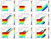 |
Fig. 1 Growth rates of unstable modes for different amplitudes of the azimuthal magnetic field for a dust-free disk with ϵ = 0 (top panel), a dust-poor disk with ϵ = 0.2 (middle panel), and a dust-rich disk with ϵ = 3. The Stokes number was fixed to St = 0.1 and the ambipolar Elsasser number to ΛAD = 100. The solid line corresponds to the RDI condition for the streaming instability (Eq. (26)), while the dashed black line corresponds to the RDI condition between Alfvén waves and the dust-gas radial drift (Eq. (29)). The dashed blue line corresponds to the condition for AD-modified Alfvén wave RDI (Eq. (39)). |
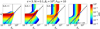 |
Fig. 2 Growth rates of unstable modes for different amplitudes of the azimuthal magnetic field. The dust-to-gas ratio was fixed to ϵ = 3, the Stokes number to St = 0.1, and the ambipolar Elsasser number to ΛAD = 10. |
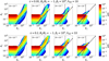 |
Fig. 3 Growth rates of unstable modes for different values of the Stokes number for ϵ = 0.01 (top) and ϵ = 0.2 (bottom). The ambipolar Elsasser number was set to ΛAD = 10 and the azimuthal field to By/Bz = −1. |
4.2 Parameter study
In this section, we discuss the dependence of the AD-driven instability described above on parameters, with a particular focus on the effect of varying the azimuthal field and the Stokes number. In Fig. 2 we display growth rates for the Lin A setup (ϵ = 3, St = 0.1) with ΛAD = 10 and for different values of By/Bz. For ![Mathematical equation: $\[B_{y}^{\prime}\]$](/articles/aa/full_html/2026/05/aa59457-26/aa59457-26-eq55.png) = −1 (second panel), the AmSI modes appear as the band of unstable modes enclosed within the region delimited by
= −1 (second panel), the AmSI modes appear as the band of unstable modes enclosed within the region delimited by ![Mathematical equation: $\[10^{2} \lesssim \tilde{K}_{x} \lesssim 10^{3}\]$](/articles/aa/full_html/2026/05/aa59457-26/aa59457-26-eq56.png) and
and ![Mathematical equation: $\[10 \lesssim \tilde{K}_{z} \lesssim 10^{2}\]$](/articles/aa/full_html/2026/05/aa59457-26/aa59457-26-eq57.png) . Compared to the case with ΛAD = 102 (bottom right panel in Fig. 1), the range of unstable modes is therefore truncated at larger wavenumbers because the ambipolar diffusivity is stronger. The smaller Elsasser number also causes the classic SI modes to appear in the blue-green rectangular region corresponding to
. Compared to the case with ΛAD = 102 (bottom right panel in Fig. 1), the range of unstable modes is therefore truncated at larger wavenumbers because the ambipolar diffusivity is stronger. The smaller Elsasser number also causes the classic SI modes to appear in the blue-green rectangular region corresponding to ![Mathematical equation: $\[1 \lesssim \tilde{K}_{x} \lesssim 10^{2}\]$](/articles/aa/full_html/2026/05/aa59457-26/aa59457-26-eq58.png) and
and ![Mathematical equation: $\[10^{2} \lesssim \tilde{K}_{z} \lesssim 10^{5}\]$](/articles/aa/full_html/2026/05/aa59457-26/aa59457-26-eq59.png) , with growth rates that increase with the amplitude of the azimuthal field because the ambipolar resistivity scales with B2, such that increasing
, with growth rates that increase with the amplitude of the azimuthal field because the ambipolar resistivity scales with B2, such that increasing ![Mathematical equation: $\[\left|B_{y}^{\prime}\right|\]$](/articles/aa/full_html/2026/05/aa59457-26/aa59457-26-eq60.png) pushes the system toward the hydrodynamic limit.
pushes the system toward the hydrodynamic limit.
Figure 3 shows the growth rates for different values of the Stokes numbers and for dust-poor disks with relatively low values ϵ = 0.01, 0.2. For ϵ = 0.01 (upper panel), the growth rates remain relatively modest, typically, with σ ≈ 10−3Ω. This case, however, (i) confirms that dust can stabilize the original oblique modes of the MRI, and it shows (ii) that the AmSI modes seem to emerge from the stable branch of these oblique modes. Because the value for ϵ is low, it seems unlikely that this is a consequence of the reduced Alfvén speed caused by dust loading. Although not shown here, we confirmed this by considering a purely magnetized gas disc, but employing an effective Alfvén speed given by
![Mathematical equation: $\[c_{A, e f f}=\frac{c_{A, z}}{\sqrt{1+\epsilon}}.\]$](/articles/aa/full_html/2026/05/aa59457-26/aa59457-26-eq61.png) (30)
(30)
For ϵ = 0.2 (lower panel), it is interesting to note that the AmSI modes can have growth rates of σ ~ 0.1Ω, even for Stokes numbers as small as St = 10−4. This suggests that in comparison with the classic SI modes, the conditions of ϵ and St for the unstable AmSI modes to develop with significant growth rates are less stringent.
5 Unstable AmSI modes
We previously identified a new branch of unstable modes that we referred to as AmSI modes. The aim of this section is to understand the origin of the different properties of these AmSI modes that emerged from our numerical calculations. In the following, we discuss in particular how dust can stabilize the oblique modes of the ambipolar-shear instability. We also demonstrate that the AmSI modes can be interpreted as arising from an RDI driven by an AD-modified Alfvén wave and the relative drift between the gas and dust components.
5.1 Effect of dust on MRI oblique modes
To investigate the effect of dust loading on the stability of the MRI oblique modes, we employed a single-fluid model of a magnetized dusty gas disk that we present in detail in Appendix A. We then used the dispersion relation that we obtained (see Eq. (A.14)) and followed Kunz & Balbus (2004) by assuming that the transition from stability to instability occurs through σ ≈ 0. In the limit σ → 0, Eq. (A.14) becomes
![Mathematical equation: $\[\sigma=-\frac{C_0}{C_1}\left(1+\frac{\Re(\mathcal{D}_1) \tau_s}{C_0}\right),\]$](/articles/aa/full_html/2026/05/aa59457-26/aa59457-26-eq62.png) (31)
(31)
where the coefficients 𝒞0 and 𝒞1 > 0 are given in Kunz & Balbus (2004, see their Eqs. (34)–(35)), and where ℜ(𝒟1) was obtained from Eq. (A.19) and reads
![Mathematical equation: $\[\mathfrak{R}(\mathcal{D}_1)=-2 f_d \frac{B_y}{B_z} \frac{k_x}{k_z}\left(c_{A, z} k_z\right)^4 \Omega+\frac{B_z^2}{\gamma \rho_i \rho_g} f_d \frac{B_y^2}{B_z^2} c_{A, z}^2 k_x^2 k_z^2 f_d \Omega^2,\]$](/articles/aa/full_html/2026/05/aa59457-26/aa59457-26-eq63.png) (32)
(32)
where fd = ϵ/(1 + ϵ). The latter expression can also be written as
![Mathematical equation: $\[\Re(\mathcal{D}_1)=-2 f_d \frac{B_y}{B_z} \frac{k_x}{k_z}\left(c_{A, z} k_z\right)^4 \Omega\left[1-\frac{\Lambda_{\mathrm{AD}}^{-1}}{2} \frac{B_y}{B_z} \frac{k_x}{k_z}\right].\]$](/articles/aa/full_html/2026/05/aa59457-26/aa59457-26-eq64.png) (33)
(33)
We note that in deriving Eq. (31), 𝒟0 was not taken into account as it is purely imaginary. For a purely magnetized gas disc, MRI oblique modes are unstable for 𝒞0 < 0 (Kunz & Balbus 2004), which requires the condition Bykx < 0 to be satisfied (Lesur 2021). In this case, it is clear that ℜ(𝒟1) > 0, which leads from Eq. (31) to a lower growth rate or even to a stabilization of the MRI oblique modes when ℜ(𝒟1) is large enough. This is fully consistent with our numerical results, which show that adding dust indeed tends to stabilize the oblique modes with high wavenumbers (see, e.g., the middle right panel of Fig. 1). Physically, this can be interpreted as resulting from the dust backreaction on the gas. It is indeed expected that this leads to a decrease in the azimuthal velocity of the gas, such that the effect of the feedback loop between ambipolar diffusion and differential rotation is weakened.
Similarly, for 𝒞0 > 0 (but still assuming Bykx < 0), Eq. (31) confirms that dust has a stabilizing effect because the term in parentheses is positive. This suggests that for small Stokes numbers and low dust-to-gas ratios, the AmSI modes that seem to originate from the stable branch adjacent to the unstable oblique modes (e.g., upper left panel of Fig. 3) are not caused by the effect of dust on the ambipolar shear instability.
5.2 AD-modified Alfvén wave RDI: No rotation
The results presented above also show a clear trend for the instability region to lie along the RDI condition for the streaming instability of Alfvén waves. To examine to which extent ambipolar diffusion causes Alfvén waves to resonate with the dust-gas drift, we first simplified the analysis presented in Sect. 3 by neglecting rotation and also considered the incompressible limit. We discuss the effect of rotation in the next section in more detail. Under these approximations, it is straightforward to show that the perturbed gas momentum and induction equations, projected along the direction of ![Mathematical equation: $\[\hat{\mathbf{n}}=\hat{\mathbf{k}} \times \hat{\mathbf{b}}\]$](/articles/aa/full_html/2026/05/aa59457-26/aa59457-26-eq65.png) , where
, where ![Mathematical equation: $\[\hat{\mathbf{k}}\]$](/articles/aa/full_html/2026/05/aa59457-26/aa59457-26-eq66.png) and
and ![Mathematical equation: $\[\hat{\mathbf{b}}\]$](/articles/aa/full_html/2026/05/aa59457-26/aa59457-26-eq67.png) are unit vectors along the directions of the k and B, respectively, leads to the following dispersion relation for the magnetic perturbations oriented along
are unit vectors along the directions of the k and B, respectively, leads to the following dispersion relation for the magnetic perturbations oriented along ![Mathematical equation: $\[\hat{\mathbf{n}}\]$](/articles/aa/full_html/2026/05/aa59457-26/aa59457-26-eq68.png) :
:
![Mathematical equation: $\[\omega^2+i \omega \gamma B^2 k^2 ~\cos ^2 \theta-k_z^2 c_{A, z}^2=0,\]$](/articles/aa/full_html/2026/05/aa59457-26/aa59457-26-eq69.png) (34)
(34)
where γ = 1/γinρiρg, θ is the angle between ![Mathematical equation: $\[\hat{\mathbf{k}}\]$](/articles/aa/full_html/2026/05/aa59457-26/aa59457-26-eq70.png) and
and ![Mathematical equation: $\[\hat{\mathbf{b}}\]$](/articles/aa/full_html/2026/05/aa59457-26/aa59457-26-eq71.png) and with σ = −iω, while magnetic perturbations oriented along
and with σ = −iω, while magnetic perturbations oriented along ![Mathematical equation: $\[\hat{\mathbf{b}}\]$](/articles/aa/full_html/2026/05/aa59457-26/aa59457-26-eq72.png) obey the following relation dispersion:
obey the following relation dispersion:
![Mathematical equation: $\[\omega^2+i \omega \gamma B^2 k^2-k_z^2 c_{A, z}^2=0.\]$](/articles/aa/full_html/2026/05/aa59457-26/aa59457-26-eq73.png) (35)
(35)
These expressions are similar to those derived by Desch (2004) and Pandey & Wardle (2008).
In the following, we restrict the study to the case of magnetic perturbations directed along ![Mathematical equation: $\[\hat{\mathbf{n}}\]$](/articles/aa/full_html/2026/05/aa59457-26/aa59457-26-eq74.png) , which correspond to classical Alfvén waves, as we show below that the instability described above can be interpreted as an RDI that is triggered when an AD-modified Alfvén wave resonates with dust. In particular, this is supported by Fig. 4, which shows for the case ϵ = 3, St = 0.1, and By/Bz = −1 the instability growth rate as a function of
, which correspond to classical Alfvén waves, as we show below that the instability described above can be interpreted as an RDI that is triggered when an AD-modified Alfvén wave resonates with dust. In particular, this is supported by Fig. 4, which shows for the case ϵ = 3, St = 0.1, and By/Bz = −1 the instability growth rate as a function of ![Mathematical equation: $\[\tilde{K}_{z}\]$](/articles/aa/full_html/2026/05/aa59457-26/aa59457-26-eq75.png) for different values of ΛAD (bottom right panel in Fig. 1), and for
for different values of ΛAD (bottom right panel in Fig. 1), and for ![Mathematical equation: $\[\tilde{K}_{x}=10^{2}, 10^{3}\]$](/articles/aa/full_html/2026/05/aa59457-26/aa59457-26-eq76.png) . As ΛAD increases, that is, as the ideal MHD regime is approached, the range of vertical modes that are unstable to pure Alfvén wave streaming instabilities is clearly recovered (bottom left panel in Fig. 1).
. As ΛAD increases, that is, as the ideal MHD regime is approached, the range of vertical modes that are unstable to pure Alfvén wave streaming instabilities is clearly recovered (bottom left panel in Fig. 1).
To clearly demonstrate that magnetic perturbations oriented along ![Mathematical equation: $\[\hat{\mathbf{n}}\]$](/articles/aa/full_html/2026/05/aa59457-26/aa59457-26-eq77.png) may be involved in the instability, we plot in Fig. 5 the velocity and magnetic field components along this direction as a function of vertical wavenumber
may be involved in the instability, we plot in Fig. 5 the velocity and magnetic field components along this direction as a function of vertical wavenumber ![Mathematical equation: $\[\tilde{K}_{z}\]$](/articles/aa/full_html/2026/05/aa59457-26/aa59457-26-eq78.png) for ϵ = 3, St = 0.1, and ΛAD = 100 (corresponding to the second panel in Fig. 2) and ϵ = 0.2, St = 0.001, and ΛAD = 10 (corresponding to the lower panel of Fig. 3). For the range of unstable vertical modes with the highest growth rates, the velocity and magnetic perturbations are essentially directed along
for ϵ = 3, St = 0.1, and ΛAD = 100 (corresponding to the second panel in Fig. 2) and ϵ = 0.2, St = 0.001, and ΛAD = 10 (corresponding to the lower panel of Fig. 3). For the range of unstable vertical modes with the highest growth rates, the velocity and magnetic perturbations are essentially directed along ![Mathematical equation: $\[\hat{\mathbf{n}}\]$](/articles/aa/full_html/2026/05/aa59457-26/aa59457-26-eq79.png) , which supports the transverse wave interpretation, whose dispersion relation is given by Eq. (34).
, which supports the transverse wave interpretation, whose dispersion relation is given by Eq. (34).
We note that this relation dispersion can also be written as
![Mathematical equation: $\[\omega^2+i \omega \eta_{\mathrm{AD}} k_z^2-k_z^2 c_{A, z}^2=0.\]$](/articles/aa/full_html/2026/05/aa59457-26/aa59457-26-eq86.png) (36)
(36)
The roots of Eq. (36) have real and imaginary parts that are given by
![Mathematical equation: $\[\Re(\omega)=c_{A, z} k_z\left(1-\frac{\eta_{\mathrm{AD}}^2 k_z^2}{4 c_{A, z}^2}\right)^{1 / 2}\]$](/articles/aa/full_html/2026/05/aa59457-26/aa59457-26-eq87.png) (37)
(37)
and
![Mathematical equation: $\[\mathfrak{J}(\omega)=-i \frac{\eta_{\mathrm{AD}} k_z^2}{2}.\]$](/articles/aa/full_html/2026/05/aa59457-26/aa59457-26-eq88.png) (38)
(38)
Solving for the resonance condition ℜ(ω) = kx(wx − vx), where ℜ(ω) is given by Eq. (37) and with vx, wx given by Eqs. (7) and (9), respectively, leads to the following relation between the vertical and radial dimensionless wavenumbers:
![Mathematical equation: $\[\widetilde{K}_z^2=\frac{2 \Lambda_{\mathrm{AD}}^2 \eta^2 \beta_z}{h^2}\left(1 \pm \sqrt{1-\frac{\widetilde{K}_x^2 \zeta_x^2}{\Lambda_{\mathrm{AD}}^2 \eta}}\right).\]$](/articles/aa/full_html/2026/05/aa59457-26/aa59457-26-eq89.png) (39)
(39)
In the limit ![Mathematical equation: $\[D \equiv \frac{\widetilde{K}_{x}^{2} \zeta_{x}^{2}}{\Lambda_{\mathrm{AD}}^{2} \eta} \ll 1\]$](/articles/aa/full_html/2026/05/aa59457-26/aa59457-26-eq90.png) , we can expand the square root to O(D2) to obtain by taking the negative solution
, we can expand the square root to O(D2) to obtain by taking the negative solution
![Mathematical equation: $\[\widetilde{K}_z^2 \approx \frac{\eta \zeta_x^2 \beta_z \widetilde{K}_x^2}{h^2}\left(1+\frac{\zeta_x^2 \widetilde{K}_x^2}{4 \eta \Lambda_{\mathrm{AD}}^2}\right),\]$](/articles/aa/full_html/2026/05/aa59457-26/aa59457-26-eq91.png) (40)
(40)
and Eq. (29) is then readily recovered in the limit of a vanishing AD resistivity.
The resonance condition given by Eq. (39) is marked by the blue line in Figs. 1, 2 and 3. For St = 0.1 (Fig. 1), the model reproduces the branch of unstable modes that appear in the By < 0 case reasonably well. For small Stokes numbers (Fig. 3), however, the agreement is less clear because the branch of unstable modes emerging from the original MRI oblique modes does not closely follow the resonance condition. To determine whether an RDI really operates in this case, we compared for each (kx, kz) the oscillation frequencies found numerically by solving the stability problem represented by Eq. (23), that is, corresponding to ℑ(σ), to the frequency expected from the resonance condition kx(wx − vx). The results of this procedure for ϵ = 0.01 and St = 0.001 are displayed in Fig. 6. It is clear that for each unstable (kx, kz) pair, the two oscillation frequencies are comparable, which seems to support the RDI interpretation.
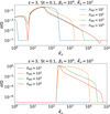 |
Fig. 4 Instability growth rate as a function of vertical wavenumber |
![Mathematical equation: $\[\tilde{K}_{z}\]$](/articles/aa/full_html/2026/05/aa59457-26/aa59457-26-eq80.png)
![Mathematical equation: $\[\tilde{K}_{x}=10^{3}\]$](/articles/aa/full_html/2026/05/aa59457-26/aa59457-26-eq81.png)
![Mathematical equation: $\[\tilde{K}_{x}=10^{2}\]$](/articles/aa/full_html/2026/05/aa59457-26/aa59457-26-eq82.png)
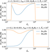 |
Fig. 5 Velocity and magnetic field components along |
![Mathematical equation: $\[\hat{\mathbf{n}}=\hat{\mathbf{k}} \times \hat{\mathbf{b}}\]$](/articles/aa/full_html/2026/05/aa59457-26/aa59457-26-eq83.png)
![Mathematical equation: $\[\tilde{K}_{z}\]$](/articles/aa/full_html/2026/05/aa59457-26/aa59457-26-eq84.png)
![Mathematical equation: $\[\tilde{K}_{x}=10^{3}\]$](/articles/aa/full_html/2026/05/aa59457-26/aa59457-26-eq85.png)
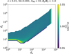 |
Fig. 6 For ϵ = 0.01 and St = 0.001, the ratio of oscillation frequencies ℑ(σ) found by solving the stability problem (Eq. (23)) and frequencies expected from the resonance condition kx(wx − vx). |
5.3 Near-resonant growth
Compared with the ideal MHD case, the results presented above suggest that the primary effect of ambipolar diffusion is to widen the range of unstable modes for which Alfvén waves can be involved in an RDI. To explain the significant width of the resonance that is obtained, we note that in presence of ambipolar diffusion, the system is almost identical to a forced oscillator, with the characteristic equation given by
![Mathematical equation: $\[\omega^2+i \omega \eta_{\mathrm{AD}} k_z^2-k_z^2 c_{A, z}^2=\omega_{R D I}^2,\]$](/articles/aa/full_html/2026/05/aa59457-26/aa59457-26-eq92.png) (41)
(41)
where we set ωRDI = kx(wx − vx), and whose oscillation amplitude 𝒜RDI would be given by
![Mathematical equation: $\[\mathcal{A}_{R D I} \propto \frac{1}{\sqrt{\left(\omega_{R D I}^2-k_z^2 c_{A, z}^2\right)^2+\left(\eta_{\mathrm{AD}} k_z^2 \omega_{R D I}\right)^2}}.\]$](/articles/aa/full_html/2026/05/aa59457-26/aa59457-26-eq93.png) (42)
(42)
The equivalent quality factor associated with this forced oscillator, which is related to the resonance width Δω through 𝒬 = kzcA,z/Δω, reads
![Mathematical equation: $\[\mathcal{Q}=\frac{c_{A, z}}{\eta_{\mathrm{AD}} k_z}=\frac{\Lambda_{\mathrm{AD}}}{\tilde{K}_z} \sqrt{\beta} h,\]$](/articles/aa/full_html/2026/05/aa59457-26/aa59457-26-eq94.png) (43)
(43)
where h is the disk aspect ratio. This corresponds to a resonant width given by
![Mathematical equation: $\[\Delta \omega=\frac{\tilde{K}_z^2}{\Lambda_{\mathrm{AD}} \beta \eta} \Omega.\]$](/articles/aa/full_html/2026/05/aa59457-26/aa59457-26-eq95.png) (44)
(44)
Setting ΛAD = 100 and h = 0.05, we obtain Q = 0.5 for ![Mathematical equation: $\[\tilde{K}_{z}\]$](/articles/aa/full_html/2026/05/aa59457-26/aa59457-26-eq96.png) = 103, such that we indeed expect the resonance to have a significant width in the presence of ambipolar diffusion. In particular, for the parameters adopted here, kzcA,z ≈ 200Ω and the resonance width is estimated to Δω ≈ 400Ω.
= 103, such that we indeed expect the resonance to have a significant width in the presence of ambipolar diffusion. In particular, for the parameters adopted here, kzcA,z ≈ 200Ω and the resonance width is estimated to Δω ≈ 400Ω.
5.4 Alfvén-modified RDI: Effect of rotation
Although the instability we found may be interpreted by the destabilization of an AD-modified Alfvén wave by the radial drift between dust and gas, it remains unclear why it disappears for Bykx > 0. We suggest that, similar to the unstable oblique modes in nonideal MHD, the instability also originates from the combination of shear and ambipolar diffusion, and thus, it can only operate under certain field geometries. In order to examine how the resonance condition given by Eq. (39) is affected by the effect of shear, we started with the dispersion relation of pure MHD waves in the presence of rotation (Kunz 2008),
![Mathematical equation: $\[\begin{aligned}& \left(\omega^2+i \omega \gamma B_z^2 k_z^2-k_z^2 c_{A, z}^2\right)\left(\omega^2+i \omega \gamma B^2 k^2-k_z^2 c_{A, z}^2\right) \\& \quad=-2 A \gamma\left(k_x B_y\right)\left(k_z B_z\right)\left[\omega^2-k_z^2 c_{A, z}^2\right],\end{aligned}\]$](/articles/aa/full_html/2026/05/aa59457-26/aa59457-26-eq97.png) (45)
(45)
where A = ∂Ω/∂ log R. To extract the effect of rotation, we searched for a correction of the AD-modified Alfvén wave frequency by writing ω = ω0 + ω1, where ω0 is given by Eq. (37) and with ω1 ∝ A. By evaluating the first derivative of the left term together with the right term of (45) with respect to ω and evaluating it at ω = ω0, and then equating terms of order A, we obtained
![Mathematical equation: $\[\omega_1=2 A i \frac{\left(k_x B_y^{\prime}\right) \gamma B_z^2}{c_{A, z}} \frac{k_z^2}{k_x^2+k^2 B_y^{\prime 2}}.\]$](/articles/aa/full_html/2026/05/aa59457-26/aa59457-26-eq98.png) (46)
(46)
Because the growth rate is σ = −iω and A < 0, an azimuthal field with orientation such that kxBy < 0 results in σ > 0, as expected. Conversely, kxBy > 0 leads to a damping of Alfvén waves through ambipolar diffusion. For kxBy > 0, we estimated under which conditions Alfvén waves are strongly damped by simply assuming ω1 = ω0 in that case. This occurs for
![Mathematical equation: $\[\Lambda_{\mathrm{AD}}<\frac{2|A| \Omega^{-1} k_x k_z B_y^{\prime}}{k_x^2+k^2 B_y^{\prime 2}}.\]$](/articles/aa/full_html/2026/05/aa59457-26/aa59457-26-eq99.png) (47)
(47)
For kx = kz and ![Mathematical equation: $\[B_{y}^{\prime}\]$](/articles/aa/full_html/2026/05/aa59457-26/aa59457-26-eq100.png) = 1, this leads to ΛAD < 1, which is consistent with what is observed in Fig. 1.
= 1, this leads to ΛAD < 1, which is consistent with what is observed in Fig. 1.
6 Direct simulations
We demonstrate the AmSI with selected axisymmetric simulations using the performance-portable Godunov code idefix (Lesur et al. 2023). To solve Eqs. (1)–(4) and (6), we enabled the MHD, dust, and shearing-box modules. We chose piecewise linear reconstruction, the HLLD Riemann solver, and a second-order Runge-Kutta time integration. Ambipolar diffusion was integrated using a Runge–Kutta–Legendre super-time-stepping scheme. We modeled a single dust species with a constant stopping time1 and included feedback onto the gas.
Our prescription for the ambipolar diffusivity in IDEFIX follows the standard form (e.g., Cui & Lin, 2021),
![Mathematical equation: $\[\left.\frac{\partial \boldsymbol{B}}{\partial t}\right|_{\mathrm{AD}, \mathrm{IDEFIX}}=\nabla \times\left[\frac{\eta_{\mathrm{AD}}^{\prime}}{|\boldsymbol{B}|^2}(\boldsymbol{J} \times \boldsymbol{B}) \times \boldsymbol{B}\right],\]$](/articles/aa/full_html/2026/05/aa59457-26/aa59457-26-eq101.png) (48)
(48)
with a constant ![Mathematical equation: $\[\eta_{\mathrm{AD}}^{\prime}\]$](/articles/aa/full_html/2026/05/aa59457-26/aa59457-26-eq102.png) . This is related to the ambipolar diffusivity used above by
. This is related to the ambipolar diffusivity used above by ![Mathematical equation: $\[\eta_{\mathrm{AD}}=\eta_{\mathrm{AD}}^{\prime} B_{z}^{2} /|\boldsymbol{B}|^{2}\]$](/articles/aa/full_html/2026/05/aa59457-26/aa59457-26-eq103.png) . At the linear level, this is only a constant factor and therefore does not affect the stability properties of the dusty gas. In Appendix B, we present code tests against the AmSI linear modes.
. At the linear level, this is only a constant factor and therefore does not affect the stability properties of the dusty gas. In Appendix B, we present code tests against the AmSI linear modes.
For the illustrative cases here, we used η = 0.05h for the radial pressure gradient and initialized the magnetic field with βz = 104, By = −Bz, and an Elsassar number ![Mathematical equation: $\[\Lambda_{\mathrm{AD}}^{\prime} \equiv c_{A, z}^{2} / \eta_{\mathrm{AD}}^{\prime} \Omega\]$](/articles/aa/full_html/2026/05/aa59457-26/aa59457-26-eq104.png) = 10. For the dust, we considered an initial ϵ = 0.2 and St = 0.01 or St = 0.1. The initial dust and gas densities are uniform, with velocities given by Eqs. (7)–(10).
= 10. For the dust, we considered an initial ϵ = 0.2 and St = 0.01 or St = 0.1. The initial dust and gas densities are uniform, with velocities given by Eqs. (7)–(10).
To isolate the AmSIs, which have short characteristic length scales, we adopted a small computational domain with x, z ∈ [−0.005, 0.005]Hg to exclude MRI-related modes. We applied periodic boundaries in z and shear-periodic boundaries in x, and we used a resolution of Nx,z = 512. The simulations were made in 3D but were axisymmetric, which was realized by setting the azimuthal domain to one cell. To trigger instability, we added random perturbations to the gas radial velocities with an amplitude of 10−3cs. Computational units were such that Hg = Ω = μ0 = 1 and the initial ρg = 1.
Figure 7 shows the evolution of the maximum gas velocity perturbations and dust-to-gas ratios for the two simulations, and Fig. 8 show snapshots of the dust-to-gas ratio. As expected, the systems are linearly unstable, with growth rates ≃0.05Ω, 0.2Ω and saturation amplitudes max |δv| ~ 3 × 10⁻⁴cs, 3 × 10⁻³cs for St = 0.01 and St = 0.1, respectively. For St = 0.01, the dust concentrations are weak, with max(ϵ) ≲ 0.3, or about an increase of 50% from the equilibrium value.
On the other hand, for St = 0.1, the dust densities can reach max (ϵ) ~ 10. The system undergoes strong oscillations, with rapid formation and destruction of transient clumps with ϵ ≳ 1 (see the right panel of Fig. 8 for an example clump). The average is max (ϵ) ≃ 2, that is, ten times the initial value. This run can be compared with the classical SI case of Johansen & Youdin (2007), who also used ϵ = 0.2 initially and St = 0.1 (their run AA), which found much lower dust overdensities of about 25%. This suggests that AmSI is more effective at concentrating dust in magnetized disks than in unmagnetized disks. However, it should be noted that MRI modes are absent by construction. The role of the AmSI in the presence of the MRI needs to be clarified in the future.
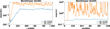 |
Fig. 7 Nonlinear evolution of the AmSI with St = 0.01 (blue) and St = 0.1 (orange). Left: maximum gas velocity perturbation. Right: maximum dust-to-gas ratio. |
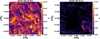 |
Fig. 8 Snapshots of the dust-to-gas ratios at the end of the AmSI simulations shown in Fig. 7. Left: St = 0.01. Right: St = 0.1. |
7 Discussion and conclusion
We examined the effect of AD on the stability of a dusty magnetized disc. The ionization fraction is expected to be relatively low in the main body of the disc, such that ambipolar diffusion is thought to play an important role in the dynamics and evolution of protoplanetary discs. In particular, it has been shown that the combined effect of ambipolar diffusion and ohmic resistivity can launch magnetically driven disk winds (Bai & Stone 2013; Gressel et al. 2015; Béthune et al. 2017) that drive accretion through the disk surfaces.
Dust feedback tends to stabilize the oblique modes of the MRI identified by Kunz & Balbus (2004). This occurs as a result of a decrease in the gas azimuthal velocity, such that the feedback loop between ambipolar diffusion and differential rotation is weakened. Depending on the orientation of the azimuthal field, our linear stability analysis also showed that ambipolar diffusion can give rise to a vigorous RDI, resulting from the destabilization of an Alfvén wave by dust-gas drift. The main effect of ambipolar diffusion is to strongly modify the Alfvén wave frequency, with the consequence that the range of wavenumbers exhibiting significant growth rates σ ≳ 0.1Ω−1 is significantly extended in comparison with a standard Alfvén wave RDI.
Our analysis showed that ambipolar diffusion has a stronger effect when the azimuthal field amplitude By is comparable to the vertical field Bz and for ambipolar Elsasser numbers ΛAD ~ 10, typically. In the outer regions of protoplanetary discs, where AD is the dominant nonideal MHD effect, ΛAD ~ 1 in the disk midplane (Bai 2011), while amplitudes of azimuthal fields such that By/Bz = 𝒪(10) were found in calculations incorporating AD (Cui & Bai 2021). Under these conditions, the requirements for efficient instability is generally not satisfied. At smaller radii R ~ 1–20 AU, however, global simulations of magnetized disk winds show that the toroidal and vertical fields can have comparable amplitudes (Bai 2017), particularly at heights Z ≲ 2H, with H the gas scale height (Gressel et al. 2015). In these inner disk regions, ΛAD is still expected to be on the order of unity, but can also be significantly higher in the presence of large grains. For example, at distances R ~ 10 AU, Simon et al. (2015) reported a value ΛAD ~ 10 at the midplane of a disk that contained 10 μm dust grains. These results therefore suggest that the instability is most likely to operate in the intermediate regions of wind-launching discs, particularly when a substantial population of large grains is present.
Interestingly, we obtained significant growth rates in dust-poor discs with ϵ ~ 0.2 and for Stokes numbers as low as St = 10−4, although numerical simulations suggest that dust enhancements resulting from unstable AmSI modes might be relatively modest in that case. For higher Stokes numbers with St = 0.1, however, we obtained more significant dust concentrations compared to an unmagnetized disc, which might facilitate planetesimal formation in magnetized discs subject to ambipolar diffusion.
A main limitation of this work is that the effect of vertical stratification was not considered. In the hydrodynamical limit and for St ~0.1, Lim et al. (2025) recently obtained good agreement between stratified and unstratified simulations of the streaming instability, such that the midplane dynamics can be well described using an unstratified setup. In a magnetized disk launching a magnetocentrifugal wind, however, AD tends to generate a flip of the toroidal field close to the disk midplane (Béthune et al. 2017). In this context, numerical simulations investigating the effect of AD on the streaming instability should ideally take into account the vertical structure of the disc. Numerical simulations of vertically global radially unstratified wind-emitting dusty discs will be presented in a future study.
Acknowledgements
Computer time for this study was provided by the computing facilities MCIA (Mésocentre de Calcul Intensif Aquitain) of the Universite de Bordeaux and by HPC resources of Cines under the allocation A0170406957 made by GENCI (Grand Equipement National de Calcul Intensif). Simulations were also carried out on the Kawas cluster at ASIAA. The authors acknowledge the access to high-performance computing facilities (Theory cluster and storage) provided by ASIAA. MKL is supported by the National Science and Technology Council (grants 113-2112-M-001-036-, 114-2112-M-001-018-, 113-2124-M-002-003-, 114-2124-M-002-003-, 115-2124-M-002-014-), an Academia Sinica Career Development Award (AS-CDA-110-M06), and an Academia Sinica Grand Challenge Seed Grant (AS-GCS-115-M02).
References
- Abod, C. P., Simon, J. B., Li, R., & et al. 2019, ApJ, 883, 192 [Google Scholar]
- Bai, X.-N. 2011, ApJ, 739, 50 [CrossRef] [Google Scholar]
- Bai, X.-N. 2017, ApJ, 845, 75 [NASA ADS] [CrossRef] [Google Scholar]
- Bai, X.-N., & Stone, J. M. 2013, ApJ, 769, 76 [Google Scholar]
- Balbus, S. A., & Hawley, J. F. 1991, ApJ, 376, 214 [Google Scholar]
- Balsara, D. S., Tilley, D. A., Rettig, T., & et al. 2009, MNRAS, 397, 24 [NASA ADS] [CrossRef] [Google Scholar]
- Béthune, W., Lesur, G., & Ferreira, J. 2017, A&A, 600, A75 [NASA ADS] [CrossRef] [EDP Sciences] [Google Scholar]
- Blum, J., & Wurm, G. 2008, ARA&A, 46, 21 [CrossRef] [Google Scholar]
- Chen, K., & Lin, M.-K. 2020, ApJ, 891, 132 [Google Scholar]
- Cui, C., & Bai, X.-N. 2021, MNRAS, 507, 1106 [NASA ADS] [CrossRef] [Google Scholar]
- Desch, S. J. 2004, ApJ, 608, 509 [Google Scholar]
- Dullemond, C. P., & Dominik, C. 2005, A&A, 434, 971 [CrossRef] [EDP Sciences] [Google Scholar]
- Goldreich, P., & Lynden-Bell, D. 1965, MNRAS, 130, 125 [Google Scholar]
- Gressel, O., Turner, N. J., Nelson, R. P., & et al. 2015, ApJ, 801, 84 [Google Scholar]
- Hopkins, P. F., & Squire, J. 2018, MNRAS, 479, 4681 [CrossRef] [Google Scholar]
- Jacquet, E., Balbus, S., & Latter, H. 2011, MNRAS, 415, 3591 [NASA ADS] [CrossRef] [Google Scholar]
- Johansen, A., & Youdin, A. 2007, ApJ, 662, 627 [Google Scholar]
- Johansen, A., Oishi, J. S., Mac Low, M.-M., & et al. 2007, Nature, 448, 1022 [Google Scholar]
- Johansen, A., Youdin, A., & Mac Low, M.-M. 2009, ApJ, 704, L75 [NASA ADS] [CrossRef] [Google Scholar]
- Kunz, M. W. 2008, MNRAS, 385, 1494 [NASA ADS] [CrossRef] [Google Scholar]
- Kunz, M. W., & Balbus, S. A. 2004, MNRAS, 348, 355 [Google Scholar]
- Laibe, G., & Price, D. J. 2014, MNRAS, 440, 2136 [Google Scholar]
- Latter, H. N., & Papaloizou, J. 2017, MNRAS, 472, 1432 [CrossRef] [Google Scholar]
- Lesur, G. 2021, J. Plasma Phys., 87, 205870101 [CrossRef] [Google Scholar]
- Lesur, G. R. J., Baghdadi, S., Wafflard-Fernandez, G., et al. 2023, A&A, 677, A9 [NASA ADS] [CrossRef] [EDP Sciences] [Google Scholar]
- Lim, J., Baronett, S. A., Simon, J. B., et al. 2025, ApJ, 993, 12 [Google Scholar]
- Lin, M.-K., & Hsu, C.-Y. 2022, ApJ, 926, 14 [NASA ADS] [CrossRef] [Google Scholar]
- Lin, M.-K., & Youdin, A. N. 2017, ApJ, 849, 129 [NASA ADS] [CrossRef] [Google Scholar]
- Nakagawa, Y., Sekiya, M., & Hayashi, C. 1986, Icarus, 67, 375 [Google Scholar]
- Pandey, B. P., & Wardle, M. 2008, MNRAS, 385, 2269 [Google Scholar]
- Sano, T., & Miyama, S. M. 1999, ApJ, 515, 776 [CrossRef] [Google Scholar]
- Simon, J. B., Lesur, G., Kunz, M. W., & Armitage, P. J. 2015, MNRAS, 454, 1117 [NASA ADS] [CrossRef] [Google Scholar]
- Simon, J. B., Armitage, P. J., Li, R., & et al. 2016, ApJ, 822, 55 [NASA ADS] [CrossRef] [Google Scholar]
- Squire, J., & Hopkins, P. F. 2018a, ApJ, 856, L15 [NASA ADS] [CrossRef] [Google Scholar]
- Squire, J., & Hopkins, P. F. 2018b, MNRAS, 477, 5011 [Google Scholar]
- Tilley, D. A., Balsara, D. S., Brittain, S. D., & et al. 2010, MNRAS, 403, 211 [NASA ADS] [CrossRef] [Google Scholar]
- Umurhan, O. M., Estrada, P. R., & Cuzzi, J. N. 2020, ApJ, 895, 4 [Google Scholar]
- Wu, Y., Lin, M.-K., Cui, C., & et al. 2024, ApJ, 962, 173 [Google Scholar]
- Yang, C.-C., Mac Low, M.-M., & Johansen, A. 2018, ApJ, 868, 27 [NASA ADS] [CrossRef] [Google Scholar]
- Youdin, A. N., & Goodman, J. 2005, ApJ, 620, 459 [Google Scholar]
- Youdin, A., & Johansen, A. 2007, ApJ, 662, 613 [Google Scholar]
- Zhuravlev, V. V. 2019, MNRAS, 489, 3850 [NASA ADS] [Google Scholar]
- Zsom, A., Ormel, C. W., Güttler, C., & et al. 2010, A&A, 513, A57 [NASA ADS] [CrossRef] [EDP Sciences] [Google Scholar]
This is equivalent to a constant Stokes number in the shearing box.
Appendix A Single-fluid model
To get insights into the effect of dust on the on the oblique modes of Kunz & Balbus (2004), we employed a more simple model of a dusty, magnetized gas. In this approach, we defined the total dust density as
![Mathematical equation: $\[\rho=\rho_g+\rho_d\]$](/articles/aa/full_html/2026/05/aa59457-26/aa59457-26-eq105.png) (A.1)
(A.1)
and the center of mass velocity as
![Mathematical equation: $\[\mathbf{u}=f_g \mathbf{v}+f_d \mathbf{w},\]$](/articles/aa/full_html/2026/05/aa59457-26/aa59457-26-eq106.png) (A.2)
(A.2)
where fg = 1/(1 + ϵ) is the gas fraction and fd = ϵ/(1 + ϵ) the dust fraction. We work within the framework of the magnetized terminal velocity approximation, which corresponds to a first order approximation in terms of the Stokes number, and which is therefore better suited to small particles. In this regime, the velocity difference between the dust and gas phases Δu = w − v is given by
![Mathematical equation: $\[\Delta \mathbf{u}=\tau_s\left[\frac{\nabla P}{\rho}-2 \eta R \Omega^2 f_g \hat{\mathbf{x}}-\frac{1}{\mu_0 \rho}(\nabla \times \mathbf{B}) \times \mathbf{B}\right]\]$](/articles/aa/full_html/2026/05/aa59457-26/aa59457-26-eq107.png) (A.3)
(A.3)
In this limit, the gas incompressibility condition, dust continuity equation, and the center-of-mass momentum equation for the dust-gas mixture are
![Mathematical equation: $\[\nabla \cdot \mathbf{u}=\nabla \cdot\left(f_d \Delta \mathbf{u}\right)\]$](/articles/aa/full_html/2026/05/aa59457-26/aa59457-26-eq108.png) (A.4)
(A.4)
![Mathematical equation: $\[\frac{\partial \epsilon}{\partial t}+\nabla \cdot(\epsilon \mathbf{u})=-\nabla \cdot \mathbf{u}\]$](/articles/aa/full_html/2026/05/aa59457-26/aa59457-26-eq109.png) (A.5)
(A.5)
![Mathematical equation: $\[\frac{\partial \mathbf{u}}{\partial t}+\mathbf{u} \cdot \nabla \mathbf{u}=-\frac{1}{\rho} \nabla P+2 \eta r \Omega^2 f_g \hat{\mathbf{x}}+2 \Omega u_y \hat{\mathbf{x}}-\frac{\Omega}{2} u_x \hat{\mathbf{y}}+\frac{1}{\mu_0 \rho}(\nabla \times \mathbf{B}) \times \mathbf{B}.\]$](/articles/aa/full_html/2026/05/aa59457-26/aa59457-26-eq110.png) (A.6)
(A.6)
In principle, the original induction equation given in Eq. 6 should be expressed in terms of u and Δu. Following Lin & Hsu (2022), we do not take this into account and simply set v → u in Eq. 6, such that the induction equation is leaved unchanged in the single fluid model. We revisit this approximation in Appendix A.4.
A.1 Linearized equations
![Mathematical equation: $\[\nabla \cdot \delta \mathbf{u}=-\frac{\sigma}{1+\epsilon} \delta \epsilon\]$](/articles/aa/full_html/2026/05/aa59457-26/aa59457-26-eq111.png) (A.7)
(A.7)
![Mathematical equation: $\[\begin{aligned}\sigma \delta \epsilon= & 2 i k_x \tau_s \eta R \Omega^2 f_g \frac{1-\epsilon}{1+\epsilon} \delta \epsilon+f_d \tau_s k^2(1+\epsilon) \frac{\delta P}{\rho} \\& +f_d \tau_s \frac{B_z}{\rho \mu_0} k^2\left(-\frac{k_x}{k_z} \delta B_x+\frac{B_y}{B_z} \delta B_y\right)\end{aligned}\]$](/articles/aa/full_html/2026/05/aa59457-26/aa59457-26-eq112.png) (A.8)
(A.8)
![Mathematical equation: $\[\sigma \delta u_x=2 \Omega \delta u_y-i k_x \frac{\delta P}{\rho}+i \frac{k^2}{k_z} \frac{B_z}{\rho \mu_0} \delta B_x-i k_x \frac{B_y}{\rho \mu_0} \delta B_y-\frac{2 \eta R \Omega^2 f_g}{(1+\epsilon)^2} \delta \epsilon\]$](/articles/aa/full_html/2026/05/aa59457-26/aa59457-26-eq113.png) (A.9)
(A.9)
![Mathematical equation: $\[\sigma \delta u_y=-\frac{\Omega}{2} \delta u_x+i k_z \frac{B_z}{\rho \mu_0} \delta B_y\]$](/articles/aa/full_html/2026/05/aa59457-26/aa59457-26-eq114.png) (A.10)
(A.10)
![Mathematical equation: $\[\sigma \delta u_z=-i k_z \frac{\delta P}{\rho}-i k_z \frac{B_y}{\rho \mu_0} \delta B_y\]$](/articles/aa/full_html/2026/05/aa59457-26/aa59457-26-eq115.png) (A.11)
(A.11)
![Mathematical equation: $\[\sigma \delta B_x=i k_z B_z \delta u_x+\frac{1}{\gamma \rho_i \rho_g}\left(-k^2 B_z^2 \delta B_x+k_x k_z B_z B_y \delta B_y\right)\]$](/articles/aa/full_html/2026/05/aa59457-26/aa59457-26-eq116.png) (A.12)
(A.12)
![Mathematical equation: $\[\begin{aligned}\sigma \delta B_y= & i k_z B_z \delta u_y-i(k_x \delta u_x+k_z \delta u_z) B_y-\frac{3}{2} \Omega \delta B_x \\& +\frac{1}{\gamma \rho_i \rho_g}(k^2 \frac{k_x}{k_z} B_z B_y \delta B_x-(k^2 B_y^2+k_z^2 B_z^2) \delta B_y)\end{aligned}.\]$](/articles/aa/full_html/2026/05/aa59457-26/aa59457-26-eq117.png) (A.13)
(A.13)
A.2 Dispersion relation
We find that the dispersion relation can be written in the form
![Mathematical equation: $\[\begin{aligned}\left(f_d \sigma^6+\mathcal{D}_5 \sigma^5+\right. & \left.\mathcal{D}_4 \sigma^4+\mathcal{D}_3 \sigma^3+\mathcal{D}_2 \sigma^2+\mathcal{D}_1 \sigma+\mathcal{D}_0\right) \boldsymbol{\tau}_s \\& +\left(\sigma^4+C_3 \sigma^3+C_2 \sigma^2+C_1 \sigma+C_0\right) \sigma=0,\end{aligned}\]$](/articles/aa/full_html/2026/05/aa59457-26/aa59457-26-eq118.png) (A.14)
(A.14)
where the coefficients 𝒞i are those given in Eqs. 32–35 of Kunz & Balbus (2004) and the coefficients 𝒟i are defined by
![Mathematical equation: $\[\mathcal{D}_5=\frac{f_d}{\gamma \rho_i \rho_g}\left(k^2 B^2+k_z^2 B_z^2\right)\]$](/articles/aa/full_html/2026/05/aa59457-26/aa59457-26-eq119.png) (A.15)
(A.15)
![Mathematical equation: $\[\begin{aligned}\mathcal{D}_4= & 2 f_d c_{A, z}^2 k_z^2+\Omega^2\left(f_d-2 i \eta R k_x\right)+\frac{3}{2} f_d \frac{B_z B_y}{\gamma \rho_i \rho_g} k_x k_z \Omega \\& +f_d\left(\frac{B B_z}{\gamma \rho_i \rho_g}\right)^2 k^2 k_z^2\end{aligned}\]$](/articles/aa/full_html/2026/05/aa59457-26/aa59457-26-eq120.png) (A.16)
(A.16)
![Mathematical equation: $\[\begin{aligned}\mathcal{D}_3= & -2 f_d \frac{B_y}{B_z}\left(c_{A, z} k_z\right)^2 \frac{k_x}{k_z} \Omega \\& +\frac{B^2 k^2+B_z^2 k_z^2}{\gamma \rho_i \rho_g}\left(f_d\left(c_{A, z} k_z\right)^2+\Omega^2\left(f_d-2 i \eta R k_x\right)\right)\end{aligned}\]$](/articles/aa/full_html/2026/05/aa59457-26/aa59457-26-eq121.png) (A.17)
(A.17)
![Mathematical equation: $\[\begin{aligned}\mathcal{D}_2= & f_d\left(c_{A, z} k_z\right)^4-\left(c_{A, z} k_z\right)^2\left(3 f_d+4 i \eta R k_x\right) \Omega^2-2 i \eta \frac{k_x k_z^2}{k^2} \Omega^4 \\& +\frac{B_z B_y}{2 \gamma \rho_i \rho_g} k_x k_z\left(3\left(f_d-2 i \eta R k_x\right) \Omega^2-f_d\left(c_{A, z} k_z\right)^2\right) \\& +\left(\frac{B B_z}{\gamma \rho_i \rho_g}\right)^2 k^2 k_z^2\left(f_d-2 i \eta R k_x\right) \Omega^2\end{aligned}\]$](/articles/aa/full_html/2026/05/aa59457-26/aa59457-26-eq122.png) (A.18)
(A.18)
![Mathematical equation: $\[\begin{aligned}\mathcal{D}_1= & -2 f_d \frac{B_y}{B_z} \frac{k_x}{k_z}\left(c_{A, z} k_z\right)^4 \Omega \\& +\frac{B_z^2}{\gamma \rho_i \rho_g}\left(\frac{B_y^2}{B_z^2}\left[\left(c_{A, z} k_x\right)^2\left(f_d-2 i \eta R k_x\right)-2 i \eta k_x\left(c_{A, z} k_z\right)^2\right] k_z^2 \Omega^2\right. \\& \left.-2 i \eta R k_x\left(1+\frac{k_z^2}{k^2}\right)\left(c_{A, z}^2 k^2+\Omega^2\right)\right)\end{aligned}\]$](/articles/aa/full_html/2026/05/aa59457-26/aa59457-26-eq123.png) (A.19)
(A.19)
Comparison of growth rates, ℜ(σ)/Ω, between IDEFIX simulations initialized with clean eigenmodes and linear theory predictions.
![Mathematical equation: $\[\begin{aligned}\mathcal{D}_0= & -2 i\left(c_{A, z} k_z\right)^2 \eta R k_x\left(\left(c_{A, z} k_z\right)^2-3 \Omega^2 \frac{k_z^2}{k^2}\right) \Omega^2 \\& -3 i \frac{B_y B_z}{\gamma \rho_i \rho_g} \eta R k_x^2 k_z\left(\left(c_{A, z} k_z\right)^2+\Omega^2 \frac{k_z^2}{k^2}\right) \\& -2 i\left(\frac{B B_z}{\gamma \rho_i \rho_g}\right)^2 \eta R k_x k_z^4 \Omega^4\end{aligned}\]$](/articles/aa/full_html/2026/05/aa59457-26/aa59457-26-eq124.png) (A.20)
(A.20)
A.3 Limit of strong nonideal effects
In the limit where ambipolar diffusion is very strong, namely for Elsasser numbers ΛA ≪ 1, an approximation to the dispersion relation can be obtained by retaining only terms ![Mathematical equation: $\[\propto \Lambda_{A}^{-2}\]$](/articles/aa/full_html/2026/05/aa59457-26/aa59457-26-eq125.png) . In this regime, we find that the dispersion relation becomes
. In this regime, we find that the dispersion relation becomes
![Mathematical equation: $\[f_g \tau_s \sigma^4+\sigma^3+\tau_s(f_d \Omega^2-2 i \eta k_x R \Omega^2)+\frac{k_z^2}{k^2} \Omega^2 \sigma-2 i k_x \tau_s \eta R \Omega^4 \frac{k_z^2}{k^2}=0\]$](/articles/aa/full_html/2026/05/aa59457-26/aa59457-26-eq126.png) (A.21)
(A.21)
which is equivalent to classical SI relation dispersion (Jacquet et al. 2011; Laibe & Price 2014; Lin & Youdin 2017). For St ≪ 1 and σ = 𝒪(St), the first term in the previous expression can be neglected, and we recover the cubic dispersion relation of Youdin & Goodman (2005).
A.4 Effective ambipolar diffusion from dust-gas drag
Recall that we neglected Δu in the induction equation for the above analysis. To evaluate the consequence of this approximation, we note that
![Mathematical equation: $\[\mathbf{v}=\mathbf{u}-f_d \Delta \mathbf{u}.\]$](/articles/aa/full_html/2026/05/aa59457-26/aa59457-26-eq127.png) (A.22)
(A.22)
It follows that the induction equation, in the ideal MHD limit, can be rewritten as
![Mathematical equation: $\[\frac{\partial \mathbf{B}}{\partial t}=\nabla \times(\mathbf{u} \times \mathbf{B})-\frac{3}{2} \Omega B_x \hat{\mathbf{y}}-\nabla \times\left(f_d \Delta \mathbf{u} \times \mathbf{B}\right).\]$](/articles/aa/full_html/2026/05/aa59457-26/aa59457-26-eq128.png) (A.23)
(A.23)
Using the magnetized terminal velocity approximation given by Eq. A.3, the previous expression becomes
![Mathematical equation: $\[\begin{aligned}\frac{\partial \mathbf{B}}{\partial t}= & \nabla \times(\mathbf{u} \times \mathbf{B})-\frac{3}{2} \Omega B_x \hat{\mathbf{y}}-\nabla \times\left[f_d \tau_s\left(\frac{\nabla P}{\rho}-2 \eta R \Omega^2 f_g \hat{\mathbf{x}}\right) \times \mathbf{B}\right] \\& +\nabla \times\left\{\tau_s f_d f_g c_A^2[(\nabla \times \mathbf{B}) \times \hat{\mathbf{b}}] \times \hat{\mathbf{b}}\right\},\end{aligned}\]$](/articles/aa/full_html/2026/05/aa59457-26/aa59457-26-eq129.png) (A.24)
(A.24)
with ![Mathematical equation: $\[c_{A}^{2}=B^{2} / \mu_{0} \rho_{g}\]$](/articles/aa/full_html/2026/05/aa59457-26/aa59457-26-eq130.png) and
and ![Mathematical equation: $\[\hat{\mathbf{b}}\]$](/articles/aa/full_html/2026/05/aa59457-26/aa59457-26-eq131.png) = B/B. Therefore, the relative drift between dust and gas phases has the same effect of the drift between neutral and charged species in MHD, as it also leads to ambipolar-like diffusion in the final term on the right hand side.
= B/B. Therefore, the relative drift between dust and gas phases has the same effect of the drift between neutral and charged species in MHD, as it also leads to ambipolar-like diffusion in the final term on the right hand side.
From the previous equation, the dust effective ambipolar resistivity would be given by ![Mathematical equation: $\[\eta_{A, \text {eff}}=\tau_{s} f_{d} f_{g} c_{A}^{2}\]$](/articles/aa/full_html/2026/05/aa59457-26/aa59457-26-eq132.png) , corresponding to an effective ambipolar Elsasser number:
, corresponding to an effective ambipolar Elsasser number:
![Mathematical equation: $\[\Lambda_{A, \mathrm{eff}}=\frac{1}{\mathrm{St} f_d f_g}.\]$](/articles/aa/full_html/2026/05/aa59457-26/aa59457-26-eq133.png) (A.25)
(A.25)
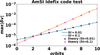 |
Fig. B.1 Evolution of the maximum gas velocity perturbations for IDEFIX runs initialized with clean eigenmodes (blue and orange curves). The stars are the expected evolution based on linear theory growth rates. |
For small grains with St ≪ 1, we have ΛA,eff ≫ 1 and thus this effect is likely unimportant compared to the true ambipolar diffusion in protoplanetary discs.
Appendix B Code test
We tested our IDEFIX setup by simulating a clean eigenmode and comparing its growth rate against linear theory. The equilibrium disk parameters are the same as that used for Sect. 6. We perturbed the equilibrium by adding axisymmetric perturbations calculated from linear theory (i.e., Eqs. 12–22 with ηAD replaced by ![Mathematical equation: $\[\eta_{\mathrm{AD}}^{\prime}\]$](/articles/aa/full_html/2026/05/aa59457-26/aa59457-26-eq134.png) ), which are characterized by wavenumbers kx,z. We normalized the perturbations so that max |δvx| = 10−6cs. We considered two cases: 1) St = 0.01 with kxHg = 4000, kzHg = 1500; and 2) St = 0.1 with kx,zHg = 1000. For these tests, the computational domain is one wavelength, that is, x, z ∈ [−π/kx,z, π/kx,z], and we use Nx,z = 128 cells in each direction.
), which are characterized by wavenumbers kx,z. We normalized the perturbations so that max |δvx| = 10−6cs. We considered two cases: 1) St = 0.01 with kxHg = 4000, kzHg = 1500; and 2) St = 0.1 with kx,zHg = 1000. For these tests, the computational domain is one wavelength, that is, x, z ∈ [−π/kx,z, π/kx,z], and we use Nx,z = 128 cells in each direction.
Figure B.1 shows the evolution of the maximum gas velocity perturbations, from which we measure growth rates over the first 8 orbits and also compare them in Table B.1. These show a good agreement between simulation and theoretical growth rates, with a relative error ≲ 1%. Not surprisingly, the St = 0.1 case, with a higher growth rate, is more accurately simulated.
The test here shows that IDEFIX is capable of capturing the AmSI. We have also reproduced growth rates with Nx,z = 64 cells at similar accuracy by using a less diffusive configuration: piecewise parabolic reconstruction, a Roe solver, and third order Runge-Kutta time integration. However, we found this setup is prone to crashing (with vanishing timesteps) when evolving the AmSI into the nonlinear regime. Hence we do not use it in Sect. 6.
All Tables
Comparison of growth rates, ℜ(σ)/Ω, between IDEFIX simulations initialized with clean eigenmodes and linear theory predictions.
All Figures
|
Fig. 1 Growth rates of unstable modes for different amplitudes of the azimuthal magnetic field for a dust-free disk with ϵ = 0 (top panel), a dust-poor disk with ϵ = 0.2 (middle panel), and a dust-rich disk with ϵ = 3. The Stokes number was fixed to St = 0.1 and the ambipolar Elsasser number to ΛAD = 100. The solid line corresponds to the RDI condition for the streaming instability (Eq. (26)), while the dashed black line corresponds to the RDI condition between Alfvén waves and the dust-gas radial drift (Eq. (29)). The dashed blue line corresponds to the condition for AD-modified Alfvén wave RDI (Eq. (39)). |
| In the text | |
|
Fig. 2 Growth rates of unstable modes for different amplitudes of the azimuthal magnetic field. The dust-to-gas ratio was fixed to ϵ = 3, the Stokes number to St = 0.1, and the ambipolar Elsasser number to ΛAD = 10. |
| In the text | |
|
Fig. 3 Growth rates of unstable modes for different values of the Stokes number for ϵ = 0.01 (top) and ϵ = 0.2 (bottom). The ambipolar Elsasser number was set to ΛAD = 10 and the azimuthal field to By/Bz = −1. |
| In the text | |
|
Fig. 4 Instability growth rate as a function of vertical wavenumber |
| In the text | |
|
Fig. 5 Velocity and magnetic field components along |
| In the text | |
|
Fig. 6 For ϵ = 0.01 and St = 0.001, the ratio of oscillation frequencies ℑ(σ) found by solving the stability problem (Eq. (23)) and frequencies expected from the resonance condition kx(wx − vx). |
| In the text | |
|
Fig. 7 Nonlinear evolution of the AmSI with St = 0.01 (blue) and St = 0.1 (orange). Left: maximum gas velocity perturbation. Right: maximum dust-to-gas ratio. |
| In the text | |
|
Fig. 8 Snapshots of the dust-to-gas ratios at the end of the AmSI simulations shown in Fig. 7. Left: St = 0.01. Right: St = 0.1. |
| In the text | |
|
Fig. B.1 Evolution of the maximum gas velocity perturbations for IDEFIX runs initialized with clean eigenmodes (blue and orange curves). The stars are the expected evolution based on linear theory growth rates. |
| In the text | |
Current usage metrics show cumulative count of Article Views (full-text article views including HTML views, PDF and ePub downloads, according to the available data) and Abstracts Views on Vision4Press platform.
Data correspond to usage on the plateform after 2015. The current usage metrics is available 48-96 hours after online publication and is updated daily on week days.
Initial download of the metrics may take a while.