| Issue |
A&A
Volume 708, April 2026
|
|
|---|---|---|
| Article Number | A198 | |
| Number of page(s) | 14 | |
| Section | Interstellar and circumstellar matter | |
| DOI | https://doi.org/10.1051/0004-6361/202558425 | |
| Published online | 10 April 2026 | |
eROSITA and STAPS study of the Antlia supernova remnant
1
Dr. Karl Remeis Observatory and Erlangen Centre for Astroparticle Physics, Friedrich-Alexander-Universität Erlangen-Nürnberg,
Sternwartstraße 7,
96049
Bamberg,
Germany
2
Department of Astrophysics/IMAPP, Radboud University,
PO Box 9010,
6500
GL
Nijmegen,
The Netherlands
3
Max-Planck-Institut für extraterrestrische Physik,
Gießenbachstraße 1,
85748
Garching,
Germany
4
Max-Planck-Institut für Radioastronomie,
Auf dem Hügel 69,
53121
Bonn,
Germany
5
Department of Astronomy, University of Science and Technology of China,
Hefei
230026,
PR
China
6
INAF – Istituto di Radioastronomia,
via P. Gobetti 101,
40129
Bologna,
Italy
7
School of Physics and Astronomy, Yunnan University,
Kunming
650500,
China
★ Corresponding author: This email address is being protected from spambots. You need JavaScript enabled to view it.
Received:
5
December
2025
Accepted:
11
February
2026
Abstract
Context. We report on the study of the Antlia supernova remnant (SNR), which is an old, nearby remnant of most likely a core-collapse supernova and which has an extent of ~24° in the sky. Since being detected in the ROSAT all-sky survey, it has not been observed in its entirety until the eROSITA all-sky survey (eRASS).
Aims. The new images of the extended ROentgen Survey with an Imaging Telescope Array (eROSITA) on board Spectrum-RG (SRG) in X-rays covering the entire SNR and its surroundings, the newest radio polarimetry data of the Southern Twenty-Centimeter All-Sky Polarization Survey (STAPS), and additional multi-wavelength data reveal the extent of the SNR and its interaction with the environment. We can thus constrain the distance and understand the evolution of the SNR.
Methods. We created mosaic images of eRASS data and extracted X-ray spectra in the entire SNR divided into smaller regions. The spectra were compared to thermal plasma models to derive the SNR’s physical properties. From the radio polarimetry data, Faraday moment maps were created and compared to optical and X-ray emission.
Results. The X-ray emission fills the interior of the shell of the Antlia SNR, which is seen in Hα and also well traced in the Faraday maps. In addition, structures are found in the extinction and Faraday maps, which are (anti-)correlated with the X-ray emission, and suggest the existence of matter in the foreground. We thus constrain the distance to 250–450 pc, yielding a lower limit that is higher than the one suggested before. The morphology in radio, optical, and X-rays suggests that the SNR is expanding in a medium with a general density gradient, as it is located above the Galactic plane. In addition, there seems to be a denser cloud at higher latitudes, with which the outer shock wave is interacting and which causes an indentation in the outer shell. The X-ray spectra suggest that the plasma in the SNR is not in collisional ionisation equilibrium, but seems to be close to equilibrium at lower Galactic latitudes. A little enhancement in Ne or S abundance is found in some regions, though the significance is low. The Faraday moment maps from the polarisation data indicate enhanced magnetic fields along the shell, with small-scale structures that coincide with small filaments in Hα.
Conclusions. By combining large-survey data of eRASS and STAPS, we have obtained a better understanding of the morphology, physical properties, and interior features of one of the closest SNRs.
Key words: ISM: general / ISM: structure / ISM: supernova remnants / radio continuum: ISM / X-rays: ISM / ISM: individual objects: Antlia SNR
© The Authors 2026
 Open Access article, published by EDP Sciences, under the terms of the Creative Commons Attribution License (https://creativecommons.org/licenses/by/4.0), which permits unrestricted use, distribution, and reproduction in any medium, provided the original work is properly cited.
This article is published in open access under the Subscribe to Open model. This email address is being protected from spambots. You need JavaScript enabled to view it. to support open access publication.
1 Introduction
Large nearby supernova remnants (SNRs) are essential for understanding the evolution and population of SNRs in the Galaxy. Due to their large extent, they are very difficult to observe as the typical field of view (FoV) of instruments can be orders of magnitude smaller in comparison. With the launch of eROSITA on board Spectrum-Roentgen-Gamma (SRG) in 2019 and the consequent all-sky surveys (eRASS), we now have the opportunity to discover these large objects and to study them in greater detail than ever before.
One of these special SNRs is the Antlia SNR, located in the same name-giving constellation at (l, b) ~ (276.5°, 19°). First discovered by McCullough et al. (2002) in Hα and in X-rays with ROSAT (Trümper 1982), the remnant has an extent of ~24°. McCullough et al. (2002) found a gamma-ray decay feature of 26Al at 1.8 MeV at the position of the SNR and the pulsar B0950+08 as a candidate for the compact object, which was produced in the supernova, although with low confidence. They derived a rather low distance, D < 240 pc, and very high age of >1 Myr for the SNR. Tetzlaff et al. (2013) re-analysed possible pulsars in the vicinity in the search for the compact object. They found PSR J0630-2834 to be a more likely candidate, based on the proper motion and its birthplace very close to the approximate centre of the SNR. Based on this, they estimate a distance of ≈111–145 pc only, and an age of ≈1.2 Myr. In the far-ultraviolet (FUV), Shinn et al. (2007) discovered features typical of radiative cooling of dense clouds hit by a powerful shock wave. They concluded that the progenitor might have exploded in a cloudy environment, leading to a mixed morphology. A recent study with GALEX FUV data by Fesen et al. (2021) revealed a striking resemblance with the Hα filaments. They also obtained optical spectra from which high [S II]/ Hα line ratios were obtained, which are typical of SNRs, supporting previous classifications of this object. Their results also suggest a shock velocity of 50–150 km/s, which indicates an age of only ~105 yr, far younger than what was previously believed. This result is in contrast with the age determined by Tetzlaff et al. (2013) from the pulsar association argument. They also discuss possible interactions with the nearby Gum Nebula (e.g., Gum 1952; Howarth & van Leeuwen 2019) that would put the remnant at distances of ≥200 pc; however, the exact geometry and extent of the nebula are still very uncertain (Fesen et al. 2021).
In this work, we perform a detailed analysis of the X-ray morphology and spectra and of radio polarimetry data of the entire Antlia SNR for the first time. With this, we can independently infer the extent of the SNR, its environment, the properties of the hot plasma, and the evolutionary properties of the SNR. In Sect. 2, we introduce the data used in this study and explain the important data reduction and processing procedures. In Sect. 3, we compare the images and discuss the extent of the SNR. In Sect. 4, we show our background study and results, on which we base our spectral analysis in Sect. 5.
2 Data
2.1 X-ray
The X-ray data were obtained with the extended ROentgen Survey with an Imaging Telescope Array (eROSITA, Predehl et al. 2021) on board SRG. We used the data of the first four all-sky surveys (eRASS 1–4, also called eRASS:4, Merloni et al. 2024) in the energy range of 0.2–10 keV. The average spatial resolution is ~26″ for eRASS, and the spectral resolution is ~80 eV at 1.49 keV. The data were analysed using the eSASS software1 (Brunner et al. 2022) version 211214 and the most recent calibration database (CalDB, Brunner et al. 2018) available at the time of processing and analysis. We used the data processed with the pipeline version 020.
The event files of all 250 sky tiles, which cover the Antlia SNR were merged, bad events and bad pixels were removed, and good-time intervals were selected. The details of the analysis are explained in Knies et al. (2024). We created images for the energy bands of 0.2–0.4 keV, 0.4–0.8 keV, and 0.8–1.25 keV, exposure maps for each of these energy bands, and exposure-corrected images.
For the spectral analysis, we extracted spectra and created response files for each analysis region (see Sect. 5). For faint diffuse emission, it is not ideal to subtract a background spectrum. Instead, we extracted the spectrum of a nearby off-source region to estimate the local X-ray background. Point and point-like sources were excluded from the data before the extraction of the spectra.
2.2 Multi-wavelength data for image comparison
We downloaded the Hα maps presented by Finkbeiner (2003) for a multi-wavelength comparison. The Hα map is a combination of data taken in the Virginia Tech Spectral line Survey (VTSS, Dennison et al. 1998), Southern H-Alpha Sky Survey (SHASSA, Gaustad et al. 2001), and the Wisconsin H-Alpha Mapper (WHAM, Reynolds et al. 2002), and has a spatial resolution of 6′. To estimate the extinction, we used the dust absorption AV data cubes of Lallement et al. (2022). We also used the data cube (Clark & Hensley 2019) of the HI4PI 21 cm neutral hydrogen (HI) survey (HI4PI Collaboration 2016) to study the distribution of the cold phase of the interstellar medium (ISM) in this region of the sky.
2.3 Radio-polarimetry data
We used radio-polarimetric data from the Southern Twenty-Centimeter All-Sky Polarization Survey (STAPS, Sun et al. 2025), at a frequency range of 1328–1768 MHz with a resolution of 1 MHz and an angular resolution of 18 arcmin. The survey was carried out using the H-OH receiver at the Murriyang telescope at Parkes, NSW, in Australia, and covers the entire sky south of 0° declination. STAPS is one of six surveys that together comprise the Global Magneto-Ionic Medium Survey (GMIMS), a comprehensive project to image both the southern and northern hemispheres in the frequency range of 300–1800 MHz to study the magnetised Galactic ISM by way of diffuse polarised synchrotron emission (Wolleben et al. 2009, 2019, 2021).
2.3.1 Faraday rotation
The linear polarisation angle, χ, of an electromagnetic wave undergoes a wavelength-dependent rotation when propagating through a magnetised, ionised medium (Burn 1966; Brentjens & de Bruyn 2005). The polarisation angle is calculated from the observable Stokes parameters, Q and U, as χ = 0.5 arctan(U/Q).
In the ISM, linearly polarised synchrotron emission and Faraday rotation co-occur. In this case, the amount of Faraday rotation, represented by the Faraday depth, ϕ, is variable for various emission components at various distances, d:
![Mathematical equation: $\[\left(\frac{\phi}{\mathrm{rad} \mathrm{~m}^2}\right)=0.812 \int_0^d\left(\frac{n_e(s)}{\mathrm{cm}^{-3}}\right)\left(\frac{\mathbf{B}(s)}{\mu \mathrm{G}}\right) \cdot\left(\frac{\mathbf{d} s}{\mathrm{pc}}\right),\]$](/articles/aa/full_html/2026/04/aa58425-25/aa58425-25-eq1.png) (1)
(1)
where ne is the thermal electron density, B the magnetic field, and ds an element of a path length out to a distance, d, of the radiation source.
Radio spectropolarimetric observations measure the complex polarisation, P(λ2), as a function of wavelength, λ, defined as
![Mathematical equation: $\[\boldsymbol{P}\left(\lambda^2\right)=P e^{2 i\left(\chi_0+\lambda^2 \phi\right)}=Q\left(\lambda^2\right)+i U\left(\lambda^2\right).\]$](/articles/aa/full_html/2026/04/aa58425-25/aa58425-25-eq2.png) (2)
(2)
From these measurements, a Faraday spectrum of polarised intensity as a function of Faraday depth, F(ϕ), can be created through a technique called rotation measure (RM) synthesis (Burn 1966; Brentjens & de Bruyn 2005):
![Mathematical equation: $\[F(\phi)=\int_{-\infty}^{+\infty} \boldsymbol{P}\left(\lambda^2\right) e^{-2 i \phi \lambda^2} d \lambda^2.\]$](/articles/aa/full_html/2026/04/aa58425-25/aa58425-25-eq3.png) (3)
(3)
In practice, limited wavelength coverage represented by a window function, W(λ2), results in an observed complex polarisation, ![Mathematical equation: $\[\tilde{P}(\lambda^{2})=W(\lambda^{2}) P(\lambda^{2})\]$](/articles/aa/full_html/2026/04/aa58425-25/aa58425-25-eq4.png) , which results in a Faraday spectrum,
, which results in a Faraday spectrum,
![Mathematical equation: $\[\tilde{F}(\phi)=K \int_{-\infty}^{+\infty} W\left(\lambda^2\right) \boldsymbol{P}\left(\lambda^2\right) e^{-2 i \phi \lambda^2} d \lambda^2=F(\phi) \boldsymbol{\star} R(\phi).\]$](/articles/aa/full_html/2026/04/aa58425-25/aa58425-25-eq5.png) (4)
(4)
Here, K = 1/ ∫ W(λ2)dλ2, ★ denotes convolution, and
![Mathematical equation: $\[R(\phi)=\int_{-\infty}^{+\infty} W\left(\lambda^2\right) e^{-2 i \phi \lambda^2} d \lambda^2\]$](/articles/aa/full_html/2026/04/aa58425-25/aa58425-25-eq6.png) (5)
(5)
is the RM spread function.
The Faraday spectrum details the amount of polarised intensity, P, at a range of Faraday depths, ϕ, for a range of distances, d. Each peak in a Faraday spectrum then indicates a source of (polarised) emission that is Faraday-rotated by a certain amount, ϕ, from which we can derive the electron-density-weighted magnetic field component along the line of sight. Sources of polarised emission in this case may be foreground and/or background synchrotron emission, and/or emission from the remnant itself.
We created Faraday spectra for the field of the Antlia SNR (Brentjens & de Bruyn 2005), resulting in a Faraday cube of sky co-ordinates versus Faraday depth that covers a ϕ range of ±750 rad m−2 in steps of 5 rad m−2. We used RM-Tools2 from the Canadian Initiative for Radio Astronomy Data Analysis (CIRADA; Purcell et al. 2020) for RM synthesis and RM-CLEAN (Heald 2009). Default parameters were adopted: a loop gain of 0.1, iterations of 1000, and the 3σ intensity cut-off per pixel (see Raycheva et al. 2025 for details).
2.3.2 Faraday moments
To simplify the interpretation of Faraday cubes, we used Faraday moment maps (Dickey et al. 2019), similar to moment maps routinely used in neutral hydrogen studies. The zeroth, first, and second Faraday moments are given by
![Mathematical equation: $\[M_0=\int_{-\infty}^{\infty} F(\phi) d \phi,\]$](/articles/aa/full_html/2026/04/aa58425-25/aa58425-25-eq7.png) (6)
(6)
![Mathematical equation: $\[M_1=\frac{1}{M_0} \int_{-\infty}^{\infty} F(\phi) \phi d \phi,\]$](/articles/aa/full_html/2026/04/aa58425-25/aa58425-25-eq8.png) (7)
(7)
![Mathematical equation: $\[M_2=\frac{1}{M_0} \int_{-\infty}^{\infty} F(\phi)\left(\phi-M_1\right)^2 d \phi.\]$](/articles/aa/full_html/2026/04/aa58425-25/aa58425-25-eq9.png) (8)
(8)
In words, the zeroth moment map shows the total polarised intensity integrated over all Faraday depths, the first moment is the polarised-intensity-weighted mean Faraday depth, and the second moment map represents the polarised-intensity-weighted width of the Faraday spectrum. A spectrum with a single unresolved peak means one polarised emission component with strength M0 at Faraday depth M1, while M2 is equal to the Faraday resolution (i.e. unresolved in Faraday depth). If the Faraday spectrum shows multiple peaks (M2 > Faraday depth resolution), this indicates either multiple emission components or a situation in which both synchrotron emission and Faraday rotation are present in the same medium.
3 Morphology
3.1 X-rays
We created a three-colour eROSITA X-ray view of the Antlia SNR and vicinity in Fig. 1. Considering the energy range, most of the emission is observed in the 0.2–0.8 keV range (red and green) and appears red or yellow. The remnant deviates from the ideal shell-like circular morphology and instead has a bowl-like shape, with the bottom of the bowl lying close to the Galactic plane. At higher Galactic latitudes we find a depression in the X-ray emission, which is consistent with the shape of the SNR seen in Hα and radio-polarimetry (see below). There are darker regions in both the eastern and western parts of the SNR. While the eastern darker region appears green in the three-colour image and suggests that the emission is absorbed by matter in the foreground, the western darker region appears red.
 |
Fig. 1 eROSITA X-ray three-colour image of the Antlia SNR for the energy bands: 0.2–0.4 keV (red), 0.4–0.8 keV (green), and 0.8–1.25 keV (blue) in Galactic co-ordinates. The image was created from the combined eRASS:4 data. The position of the SNR is marked by the yellow region. |
 |
Fig. 2 Hα image of Antlia SNR (Finkbeiner 2003). The position of the SNR is marked by the yellow region. |
3.2 Hα
The Hα emission is shown in Fig. 2. The structure seen in Hα is consistent with the diffuse X-ray emission and traces the edges of the remnant well. It suggests that the SNR is located at the outer edge of the Galactic disk with a significant density gradient. However, there also seems to be an obstacle above the Galactic plane, which has prevented the SNR from expanding freely to higher latitudes.
3.3 Radio-polarimetry
The Faraday moment maps are shown in Fig. 3, where the second moment mapped is root-normalised ![Mathematical equation: $\[m_{2}=\sqrt{M_{2}}\]$](/articles/aa/full_html/2026/04/aa58425-25/aa58425-25-eq10.png) . In all three Faraday moment maps, one can identify the outer boundaries of the SNR, consistent with the bowl shape in X-rays and Hα. The low-latitude boundary shows depolarisation in the M0 map where Antlia overlaps with the Gum Nebula, coincident with the bright Hα filament in Fig. 2. At the eastern edge, a region of enhanced positive Faraday depth is visible in the M1 map, which is identified as a high-RM region in Purcell et al. (2015), who named it the ‘stalk’ and suggested that this could be a blow-out of ionised material from a hole in the Gum Nebula shell. All three moment maps show that the Faraday depth structure inside of the Antlia SNR is markedly more mottled and small-scaled than around the remnant, indicating fluctuations in electron density and/or magnetic field on smaller scales inside than around the SNR. The lack of X-ray emission at the north-eastern edge seems to coincide with a patch of high positive Faraday depth, while the boundary between high and low X-rays in the SNR’s south-west denotes the boundary between positive and negative Faraday depths. However, due to the abundance of small-scale structure, it is hard to determine if a correlation between the dark patches in X-rays and structure in radio is actually present.
. In all three Faraday moment maps, one can identify the outer boundaries of the SNR, consistent with the bowl shape in X-rays and Hα. The low-latitude boundary shows depolarisation in the M0 map where Antlia overlaps with the Gum Nebula, coincident with the bright Hα filament in Fig. 2. At the eastern edge, a region of enhanced positive Faraday depth is visible in the M1 map, which is identified as a high-RM region in Purcell et al. (2015), who named it the ‘stalk’ and suggested that this could be a blow-out of ionised material from a hole in the Gum Nebula shell. All three moment maps show that the Faraday depth structure inside of the Antlia SNR is markedly more mottled and small-scaled than around the remnant, indicating fluctuations in electron density and/or magnetic field on smaller scales inside than around the SNR. The lack of X-ray emission at the north-eastern edge seems to coincide with a patch of high positive Faraday depth, while the boundary between high and low X-rays in the SNR’s south-west denotes the boundary between positive and negative Faraday depths. However, due to the abundance of small-scale structure, it is hard to determine if a correlation between the dark patches in X-rays and structure in radio is actually present.
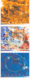 |
Fig. 3 Faraday moments M0 (in Krad m−2, top), M1 (in rad m−2, middle), and |
![Mathematical equation: $\[m_{2}=\sqrt{M_{2}}\]$](/articles/aa/full_html/2026/04/aa58425-25/aa58425-25-eq11.png)
3.4 Dust distribution
In order to trace the dust distribution, we created images of the dust extinction, AV, from Lallement et al. (2022) and overlaid them on the X-ray mosaic. In addition, we compared the X-ray and radio emission to the dust map created by Edenhofer et al. (2024) as shown in Fig. 4.
The dust at distances up to ~200 pc appears to be correlated with the X-ray brightness depression and hardening in the east and in the centre (left). In the north, there is a diffuse cloud at ~250pc, which correlates with the indentation seen in the SNR (middle). The dust at >430 pc seems to cause absorption of X-rays in the west and at lower latitudes, while there is no obvious correlation with the SNR.
4 X-ray background study
4.1 Motivation
As one can see in the X-ray images, there is also significant diffuse emission outside the SNR. Therefore, the analysis of the SNR emission requires an accurate consideration of the X-ray background. In particular, careful modelling of the background components is crucial for the spectral analysis. Moreover, due to the large extent of the SNR, the X-ray background might vary strongly across different parts of the object. As shown in our study for the similarly large Monogem Ring SNR (Knies et al. 2024), the background varies significantly, especially along the Galactic latitude. We adopted our successful approach from Knies et al. (2024) and defined background regions all around the source to be able to obtain an accurate background model for each position inside the source by averaging the closest background regions. Our regions were chosen so that as little as possible contamination by other sources was included, while having enough statistics.
4.2 Model
We largely adopted the model in Knies et al. (2024) but improved the description of the Galactic absorption. The most important components are briefly discussed again below. For the entire spectral analysis, we used the solar abundances reported by Wilms et al. (2000).
First, we accounted for the local hot bubble (LHB) with an unabsorbed APEC3 model for thermal emission from collisionally ionised plasma with a temperature of 0.09–0.13 keV, based on the studies by Liu et al. (2017); Yeung et al. (2023). Next, we introduced absorbed components to account for Galactic and extragalactic components. For the absorption component, we used the DISNHT model of Locatelli et al. (2022), which implements a log-normal distribution of NH values to construct a table model. We used the cross-sections and abundances reported in Wilms et al. (2000) and the NH values from the HI4PI survey (HI4PI Collaboration 2016). We sampled the HI4PI map with a pixel size of 8′ × 8′ and then separately calculated a DISNHT table model for each background region. We multiplied the DISNHT model with the additive background components discussed in the next paragraph.
We accounted for the emission from the circumgalactic medium (CGM) with an APEC that has a temperature close to the virial temperature of the Milky Way of kT = 0.15–0.25 keV (Gupta et al. 2021; Ponti et al. 2023). The abundance of this component was fixed to sub-solar abundances, Z ~ 0.11 Z⊙ (Fukugita & Peebles 2006; Bregman et al. 2018; Ponti et al. 2023), consistent with previous studies. We used a second Galactic component for the X-ray emission attributed to the ‘elusive Galactic corona’ based on the results of Ponti et al. (2023). This component is described by an APEC model with a higher temperature fixed to kT = 0.7 keV (Yoshino et al. 2009; Gupta et al. 2021; Ponti et al. 2023; Locatelli et al. 2024). Lastly, we accounted for the (unresolved) extragalactic background with a double-broken power-law model, BKN2POW, using Γ1 = 1.96 for E < 0.6 keV, Γ2 = 1.75 for 0.6 < E < 1.2 keV, and Γ3 = 1.45 for E > 1.2 keV, based on the ‘CXBs’ model of Ponti et al. (2023).
To account for contamination at the Lagrange 2 point, at which eROSITA is located, due to solar wind charge exchange (SWCX) we also introduced the ‘AtomDB Charge Exchange Model v2.0’ (ACX2, Smith et al. 2012; Foster et al. 2020)4 (v1.1.0) model component. We fixed the wind velocity to a typical 450 km/s based on previous studies (Cumbee et al. 2018; Zhang et al. 2022) and considered a single recombination for the emission process.
In summary, we have the following model expression in xspec for the background emission:
![Mathematical equation: $\[\begin{aligned}& \mathrm{CONST}_{\mathrm{cal}} \times \mathrm{CONST}_A \times\left(\mathrm{ACX}_{\mathrm{SWCX}}+\mathrm{APEC}_{\mathrm{LHB}}\right. \\& \left.+\mathrm{DISNHT} \times\left(\mathrm{APEC}_{\mathrm{CGM}}+\mathrm{APEC}{ }_{\text {Corona }}+\mathrm{BKN} 2 \mathrm{POW}_{\mathrm{CXB}}\right)\right).\end{aligned}\]$](/articles/aa/full_html/2026/04/aa58425-25/aa58425-25-eq12.png) (9)
(9)
The constant factor, CONSTcal, takes into account that there might be slight differences in the normalisation of the different telescope modules (TMs). This value was fixed to 1 for TM1. CONSTA is used to scale for the analysed area, A, and is necessary for the analysis of the source emission in the next step. In addition to the X-ray background, we also modelled the detector background based on the filter-wheel closed data. We adopted the model derived by Yeung et al. (2023). The details of the model are described in Appendix A by Yeung et al. (2023). We multiplied this model by a scaling constant to account for different detector areas of our spectral extraction regions. The details of the spectral fitting routine is given in Knies et al. (2024). Two example spectra with models are shown in Fig. A.1 in a region close to the plane (Fig. A.1a) and at higher latitudes (Fig. A.1b).
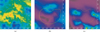 |
Fig. 4 Dust map derived by Edenhofer et al. (2024), integrated in the distances of (a) 150–190 pc, (b) 230–270 pc, and (c) 430–490 pc with the outlines of the SNR. |
4.3 Results
We show the results of the spectral analysis of the background regions with this model in Fig. A.2 in Appendix A. We obtained very good fits with this model, with cstat/d.o.f. = 0.96–1.12 (Fig. A.2a). Since the Galactic components vary strongly with the distance from the Galactic plane, we discuss the results in relation to the Galactic latitude.
The LHB appears to be roughly uniform for b > 10° (Fig. A.2b). Towards lower latitudes we obtain a higher normalisation, albeit with relatively high uncertainties. The median is given as ηLHB = ![Mathematical equation: $\[1.06_{-0.10}^{+0.07}\]$](/articles/aa/full_html/2026/04/aa58425-25/aa58425-25-eq13.png) · 10−6 cm−5 arcmin−2. The normalisation can be converted to the emission measure (EM) with
· 10−6 cm−5 arcmin−2. The normalisation can be converted to the emission measure (EM) with
![Mathematical equation: $\[\mathrm{EM}=\frac{\eta}{2.081 \cdot 10^{-4}}=5.09 \cdot 10^{-3}\left[\mathrm{~cm}^{-6} \mathrm{pc}\right]\]$](/articles/aa/full_html/2026/04/aa58425-25/aa58425-25-eq14.png) (10)
(10)
(Knies et al. 2024). This is slightly lower than what is reported in Liu et al. (2017); however, their results might include some contamination by the Antlia SNR since they obtained an enhancement in the EM of the LHB in the direction of the Antlia SNR. If we consider the surrounding EM, the results appear to be consistent.
The path length through the LHB is 166 pc in the direction of Antlia’s centre according to the model by O’Neill et al. (2025). Assuming a volume filling factor of f = 1 for the hot gas, the EM above implies a thermal electron density of ne = 0.0055 cm−3, in agreement with earlier estimates from X-ray emission (Snowden et al. 2014).
The CGM temperature is consistent across the different regions and centred around kT ~ 0.18 keV. Similar results were obtained in the study by Ponti et al. (2023). This agrees well with the theoretical virial temperature (Gupta et al. 2021). For the normalisation, we obtained a median of ηCGM = ![Mathematical equation: $\[8.76_{-1.05}^{+0.94}\]$](/articles/aa/full_html/2026/04/aa58425-25/aa58425-25-eq15.png) . 10−6 cm−5 arcmin−2. Towards the Galactic plane for b < 10°, we obtain a significantly higher normalisation, which confirms that we indeed describe a Galactic component with our model. For the hot corona component, we also measured a similar increase towards the Galactic plane; however, with a slightly different shape. When compared to theoretical mass profiles at the position of the Antlia SNR along Galactic latitude, our normalisation takes a strikingly similar trend. This indicates that indeed the hot corona component is of a Galactic origin. In general, this component is weaker by at least an order of magnitude compared to the CGM component, with the median of ηCor =
. 10−6 cm−5 arcmin−2. Towards the Galactic plane for b < 10°, we obtain a significantly higher normalisation, which confirms that we indeed describe a Galactic component with our model. For the hot corona component, we also measured a similar increase towards the Galactic plane; however, with a slightly different shape. When compared to theoretical mass profiles at the position of the Antlia SNR along Galactic latitude, our normalisation takes a strikingly similar trend. This indicates that indeed the hot corona component is of a Galactic origin. In general, this component is weaker by at least an order of magnitude compared to the CGM component, with the median of ηCor = ![Mathematical equation: $\[1.17_{-0.31}^{+0.26}\]$](/articles/aa/full_html/2026/04/aa58425-25/aa58425-25-eq16.png) · 10−7 cm−5 arcmin−2.
· 10−7 cm−5 arcmin−2.
Finally, the extragalactic background is best fit with ηCXB = ![Mathematical equation: $\[8.14_{-0.27}^{+0.20}\]$](/articles/aa/full_html/2026/04/aa58425-25/aa58425-25-eq17.png) · 10−7 photons/keV/cm2. This is consistent with the typical results for the CXB (e.g., Kuntz & Snowden 2000; Snowden et al. 2008). However, the normalisation appears to be systematically enhanced beyond the individual uncertainties of the normalisation for background regions with l < 280° by up to ~20%. Whether this increase is real or an artefact of our fixed power-law indices is difficult to judge. When excluding point-source candidates while keeping the indices fixed might result in a different normalisation, we would expect no systematic offset due to this, since we apply the same criteria for every background region. Therefore, this could indicate a localised enhancement in the CXB.
· 10−7 photons/keV/cm2. This is consistent with the typical results for the CXB (e.g., Kuntz & Snowden 2000; Snowden et al. 2008). However, the normalisation appears to be systematically enhanced beyond the individual uncertainties of the normalisation for background regions with l < 280° by up to ~20%. Whether this increase is real or an artefact of our fixed power-law indices is difficult to judge. When excluding point-source candidates while keeping the indices fixed might result in a different normalisation, we would expect no systematic offset due to this, since we apply the same criteria for every background region. Therefore, this could indicate a localised enhancement in the CXB.
4.4 Application to the spectral analysis
We adopted our approach from Knies et al. (2024) and constructed a background model for each of the source regions based on our results presented above. We summarise the most important steps as follows.
For each source region, we calculated the angular separation in Galactic latitude and selected the four background regions with the least separation. We then weighed the relevant background model fit parameters, including the 90% confidence interval (CI), based on
![Mathematical equation: $\[\bar{x}=\frac{\sum_{i=1}^n w_i x_i}{\sum_{i=1}^n w_i},\]$](/articles/aa/full_html/2026/04/aa58425-25/aa58425-25-eq18.png) (11)
(11)
where the weights were defined as 1/wi = 2dgal,b,i + dabs,i with a distance in Galactic latitude of dgal,b,i and an absolute angular distance of dabs,i between the source and background region (Knies et al. 2024). From this, we calculated ranges for each background model parameter for each source region separately. For the source model, we then constrained the background model to the aforementioned parameter ranges and add our source components. Since the SWCX contamination can vary on short timescales between different scans of eROSITA and consequently between different regions, we treated the ACX2 model parameters differently. For the SWCX contamination, we took the mean normalisation and temperatures obtained for all background regions, including the 90% CI, given as ηACX2 = ![Mathematical equation: $\[5.82_{-4.82}^{+8.68}\]$](/articles/aa/full_html/2026/04/aa58425-25/aa58425-25-eq19.png) · 10−5 cm−5 and kTACX2 =
· 10−5 cm−5 and kTACX2 = ![Mathematical equation: $\[0.154_{-0.064}^{+0.021}\]$](/articles/aa/full_html/2026/04/aa58425-25/aa58425-25-eq20.png) . While still constrained to a relatively narrow range, this allowed for more freedom during the fit to account for solar activity variations.
. While still constrained to a relatively narrow range, this allowed for more freedom during the fit to account for solar activity variations.
 |
Fig. 5 Contour-bin map where each distinct colour represents a contour-bin region, used for extracting individual spectra. The green × symbol marks the location of the associated bin in the example spectrum shown in Fig. 8. |
5 X-ray spectral analysis
5.1 Spectral analysis regions
With a good description of the background, we focused on the source regions of the Antlia SNR next. We used two different methods to define spectral extraction regions. In the first approach, we defined the regions purely on the count-based statistic of the X-ray data, using the contour-bin method of Sanders (2006). Here, all regions had to meet the minimum signal-to-noise ratio (S/N) of ~200 and in total, we obtained 92 bins with a mean S/N of 234. At the same time, this method takes the morphology into account, which we view as a benefit over the similar Voronoi-binning method (Cappellari 2009), which sometimes lead to extraction regions with very inconsistent plasma conditions. The statistics were calculated based on the point-source subtracted eROSITA counts image in the 0.2–1.25 keV energy range, where the Antlia SNR is the brightest. The resulting contour-bin map is shown in Fig. 5.
The second method was to define the regions by hand, based on the X-ray, Faraday rotation, and Hα morphology as shown in Fig. 6. We defined parts of the source with seemingly similar colour or emission characteristics as regions, while at the same time keeping the limited statistics of the data in mind. This allowed for larger regions with similar properties for a more in-depth study.
5.2 Spectral model
In addition to the background model with individually precalculated parameter ranges for each region, we first added the following components to the model to account for the emission from the SNR: TBABS × VNEI. The VNEI model describes a thermal plasma in different collisional ionisation states, also allowing for variable abundances (Hamilton et al. 1983; Borkowski et al. 1994; Liedahl et al. 1995; Borkowski et al. 2001), while the TBABS model allows for possible interstellar absorption in the foreground (Wilms et al. 2000). We limited the analysis of the contour-bin regions to this relatively simple model with solar abundances due to the smaller regions. For the manually defined regions, we have better statistics that allowed us to vary elements characteristic for SNRs and obtain a deeper insight into the plasma conditions.
 |
Fig. 6 Manually defined spectra extraction regions overlayed on the X-ray mosaic shown in Fig. 1. The labels are abbreviations for the region names given in Table 1. In addition, an ellipse region is shown that covers the entire SNR and is used for calculations of physical parameters of the SNR in Sect. 7.2. |
5.3 Results
5.3.1 Contour binning
For the contour bins, we obtained the results shown in Fig. 7 with the simple TBABS × NEI model. We obtained a very good description of the emission using this model, with cstat/d.o.f. = cstat/1749 = 0.97–1.19 (Fig. 7a). We show an example spectrum in Fig. 8.
The emission seems to be well described with a rather low mean temperature of kT = ![Mathematical equation: $\[0.19_{-0.07}^{+0.26}\]$](/articles/aa/full_html/2026/04/aa58425-25/aa58425-25-eq21.png) for the bins inside the SNR shown with a yellow region in Fig. 7b. The higher-temperature bins coincide with the darker region marked as the ‘large_E (lE)’ region shown in Fig. 6. Its X-ray colour appears to be bluer, and thus the emission to be harder compared to the surroundings. The bins in the centre are fitted with low temperatures of 0.10–0.15 keV, which is consistent with the remnant being relatively old.
for the bins inside the SNR shown with a yellow region in Fig. 7b. The higher-temperature bins coincide with the darker region marked as the ‘large_E (lE)’ region shown in Fig. 6. Its X-ray colour appears to be bluer, and thus the emission to be harder compared to the surroundings. The bins in the centre are fitted with low temperatures of 0.10–0.15 keV, which is consistent with the remnant being relatively old.
For the ionisation timescale, τ, shown in Fig. 7c, we observe a strong gradient, with lower timescales rather in the centre and at higher latitudes. The bins at lower latitudes have higher τ (appearing red to white in the parameter map), and thus are close to or consistent with collisional ionisation equilibrium (CIE). This trend also extends towards the west (right-hand side).
Finally, the normalisation is shown in Fig. 7d and shows a similar trend as the ionisation timescale, τ. This is consistent with the density distribution, which increases towards lower latitudes, and can also be seen in the Hα data (Fig. 2).
5.3.2 Manually defined regions
Next, we performed a more detailed spectral analysis with the manually defined regions to follow up on our interesting findings. Due to the higher statistics of the manually defined regions shown in Fig. 6, we were able to also investigate the elemental abundances in more detail. We used the fitting method described in Appendix C in Knies et al. (2024). In short, we tested whether the SNR characteristic elements (O, Ne, Mg, Si, S, and Fe) were consistent with solar, and if not we tested if letting the specific elements free yielded a significant (3σ) improvement of the fit.
The results of our spectral analysis are given in Table 1. We only obtained significant non-solar abundances for the elements O, Ne, S, and Fe. For about half of the regions, freeing and fitting the abundances did not improve the fit significantly. The model describes the diffuse X-ray emission well, with cstat/d.o.f. = 1.06–1.24. Two example spectra are shown in Fig. 9, where we show spectra from the ‘central_SE’ and ‘large_E’ regions.
The interesting region large_E, where the contour-bin results showed different plasma properties, also appears different in this analysis. It has the highest temperature together with the neighbouring ‘central_NE’ region – with kT = ![Mathematical equation: $\[0.28_{-0.04}^{+0.03}\]$](/articles/aa/full_html/2026/04/aa58425-25/aa58425-25-eq22.png) keV and kT =
keV and kT = ![Mathematical equation: $\[0.31_{-0.06}^{+0.07}\]$](/articles/aa/full_html/2026/04/aa58425-25/aa58425-25-eq23.png) keV. This agrees with the temperature enhancement observed in Fig. 7b. In those two regions, we also obtain a similarly enhanced S abundance, while O and Ne are not. In Appendix B, we show the confidence contours for the fit parameters for temperature kT, Ne, and S abundances for these two regions. In central_NE, the Fe also appears to be enhanced. In general, there appears to be a trend of higher abundances towards heavier elements, and Ne and S especially appear to be enhanced. We show the ratio with Fe in Fig. 10, which indicates a ratio of X/Fe < 1; however, the uncertainties are too large for a definitive claim.
keV. This agrees with the temperature enhancement observed in Fig. 7b. In those two regions, we also obtain a similarly enhanced S abundance, while O and Ne are not. In Appendix B, we show the confidence contours for the fit parameters for temperature kT, Ne, and S abundances for these two regions. In central_NE, the Fe also appears to be enhanced. In general, there appears to be a trend of higher abundances towards heavier elements, and Ne and S especially appear to be enhanced. We show the ratio with Fe in Fig. 10, which indicates a ratio of X/Fe < 1; however, the uncertainties are too large for a definitive claim.
6 Radio-polarimetric analysis
Radio emission from the Antlia SNR is only detected at the south-eastern edge in the Haslam et al. (1982) survey at 408 MHz, as noted in McCullough et al. (2002). The preprocessed (source-subtracted and de-striped) map of the same basic data (Remazeilles et al. 2015), given in Fig. 11 shows a shell-like structure coinciding with the extent of the SNR seen in X-rays and the polarimetry data, while there is a dearth of emission near the centre of the remnant, suggesting a limb-brightening effect.
The SNR stands out clearly in polarimetric data. The Faraday moment maps show the following details:
M0.. The zeroth Faraday moment (total polarised intensity at every Faraday depth) shows a mottled structure inside Antlia, for a part coinciding with Hα filaments (Fig. 2). Fluctuations in the thermal electron density cause variations in Faraday rotation; if this happens on sub-beam scales, the beam is partially or completely depolarised, visible as the black(-ish) filaments in the M0 map. Some of the narrower Hα filaments are visible as depolarised filaments in M0; others are not. The Hα causing depolarised filaments must lie at the near edge of the remnant, while the polarised emission is from either the remnant itself or the background. The Hα filaments that do not cause depolarisation must be located at the far edge of the remnant, proving that the polarised emission is generated (at least in a large part) inside the SNR itself. A large filament of remarkable constant polarised intensity is visible at the southern edge, exactly coinciding with a large and uniform Hα feature. The uniformness of M0 indicates that the magnetic field in that filament needs to be uniform as well.
M1.. The first Faraday moment (mean Faraday depth weighted by polarised intensity) shows positive and negative values, indicating an averaged line-of-sight magnetic field component ⟨B∥⟩ pointing towards and away from us, respectively (see Eq. (1)). Higher Faraday depths, M1, tend to agree with higher Hα, as the Faraday depth is proportional to the thermal electron density. However, sign changes in M1 always indicate a sign change in parallel magnetic field component. The background appears to contain a large-scale reversal in the sign of B∥, possibly due to a magnetic field mostly in the plane of the sky with a small curvature. This background Faraday depth seems to be altered by adding small-scale structure inside the remnant. In particular, B∥ changes direction along the western edge of the remnant, possibly indicating a compressed magnetic field along the shell as predicted by analytical theory and numerical simulations (Wityk et al. 2009; West et al. 2016).
M2.. The second moment, equivalent to the width of the Faraday spectrum weighted by polarised intensity, shows the smallest values in the surroundings of the SNR in the west at high latitudes, consistent with a single unresolved Faraday component. Inside the remnant, enhanced M2 values indicate a broader Faraday spectrum, especially in the southern half of the remnant, where most of the X-ray emission is. This could be due to one Faraday-thick component (a broader structure of both synchrotron emitting and Faraday rotating gas), or multiple components. As the structure in M2 (and M1) seems to morphologically correlate with the X-rays, at least one of these components is due to the remnant.
In each of the Faraday moments M0, M1, and M2, the structure inside the SNR is much patchier than the surroundings. The patchiness of Faraday depths is at least partially due to the small-scale filamentary structure in electron density as traced by the Hα, but may carry imprints of small-scale magnetic field structure as well.
 |
Fig. 7 Spectral analysis results with the contour-binning method, using the TBABS × NEI model for the source emission, in Galactic co-ordinates. In (a) we show the reduced χ2 for the fit, in (b) the plasma temperature, kT, in keV, in (c) the ionisation timescale, τ in cm−3 s, and in (d) the normalisation of the plasma component, normalised to the respective area of the bins for comparability, in cm−5 arcmin−2. The approximate outline of the Antlia SNR is indicated by a yellow region. |
Spectral fit results.
 |
Fig. 8 Example spectrum for the bin #26, located at the indicated position in Fig. 5. The thick dotted line shows the source component. The lower panel shows the residuals. For visual purposes only, the spectra were binned with a minimum of 5σ or 50 counts per bin and for better visibility only the spectrum and model for TM1 is shown. |
7 Discussion
7.1 Extinction and distance estimates
From the spectral analysis, we obtained information about the conditions of the X-ray emitting plasma, which we can use to infer properties of the entire SNR. In Sect. 3 we described the depression in brightness and hardening of the X-ray emission to the Galactic east, covered with the ‘large_E’ spectral analysis region. We extracted the dust extinction profile using the EXPLORE: G-Tomo app5 based on the Lallement et al. (2022) data cubes at (l, b) = (283°, 20°) and in the X-ray bright central part of the SNR at (l, b) = (277°, 20°) (Fig. 12). We converted the extinction, AV, at the position in large_E with obvious foreground absorption to the equivalent column density, NH, using
![Mathematical equation: $\[N_{\mathrm{H}, \mathrm{X}}=A_J \cdot 7.2( \pm 0.5) \cdot 10^{21} \mathrm{~cm}^{-2}\]$](/articles/aa/full_html/2026/04/aa58425-25/aa58425-25-eq104.png) (12)
(12)
with the conversion factor AJ = AV · ![Mathematical equation: $\[0.34_{-0.04}^{+0.02}\]$](/articles/aa/full_html/2026/04/aa58425-25/aa58425-25-eq105.png) (Vuong et al. 2003; Knies et al. 2024).
(Vuong et al. 2003; Knies et al. 2024).
The dust maps (Fig. 4) and the profile (Fig. 12) suggest that there is denser material in front of the SNR up to a distance of ~200 pc, which roughly corresponds to the extent of the Local Bubble. At D = 300 pc we obtain a column density equal to ~0.03 · 1022 cm−2, which is consistent with the upper limit of NH < 0.05 · 1022 cm−2 for the large_E region. This is consistent with the onset of the Local Bubble wall at a range of distances of ~160 pc to ~190 pc across the SN in the model by O’Neill et al. (2024) and a similar distance in the Lallement et al. (2022) analysis in Fig. 12. Moreover, we find a cloud in the north at a distance of D = 230 − 270 pc, which is anti-correlated with the SNR (Fig. 4b), suggesting that the indentation of the SNR is caused by this cloud.
 |
Fig. 9 Example spectra of the (a) central_SE and (b) large_E regions. The lower panel shows the residuals. For visual purposes only, the spectra were binned with a minimum of 5σ or 50 counts per bin and for better visibility only the spectrum and model for TM1 is shown. |
7.2 Properties of the SNR
Based on the spectral analysis, we can estimate the evolutionary parameters of the SNR. We adopted the method in Knies et al. (2024), whereby we calculated SNR models and compared them to our spectral analysis results.
First, we defined a geometry for the SNR. We simplified the geometry by using an ellipsoid as shown in Fig. 6, which included most of the area what we considered to be part of Antlia SNR. The ellipse had a semi-major axis of a = 13.5° and a semi-minor axis of b = 11.7°. We assumed that the projected semi-axis of the ellipsoid was equal to the semi-major axis, a, as the SNR seems to be distorted mainly to higher latitudes.
The density was estimated from the normalisation of our spectral fits as in Knies et al. (2024). The EM was estimated using
![Mathematical equation: $\[\mathrm{EM}=\eta \cdot\left(\frac{10^{-14}}{4 \pi D^2}\right)^{-1}=\int n_{\mathrm{e}} n_{\mathrm{H}} f d V,\]$](/articles/aa/full_html/2026/04/aa58425-25/aa58425-25-eq106.png) (13)
(13)
with the volume, V, the filling factor, f, and ne, nH being the electron and hydrogen densities of the plasma, respectively (Hamilton et al. 1983; Kavanagh et al. 2022; Knies et al. 2024). Finally, we approximated the pre-shock density using ne/nH = 1.21 and n0 ≈ 1.1 nH,0 (Kavanagh et al. 2022). Additionally, we constrained the SNR evolutionary parameter space by comparing our derived X-ray temperature with the predicted model temperature.
We used a modified version of SNRpy by Leahy et al. (2017) to facilitate calculating a grid of SNR models assuming different ages, ISM densities, and explosion energies. We used the explosion energy range E0 = (0.1–2.0) · 1051 erg based on simulations (Müller et al. 2016). For the ISM density we used n0 = 0.3 · 10−3 − 0.06 cm−3, for which the upper limit was based on the study by Elwood et al. (2017). As the lower limit, we used the density derived for the X-ray emitting plasma from the contour-bin spectral analysis results as shown in Fig. 7. We used the normalisation values in the SNR region indicated in Fig. 7d. For each distance we calculated the density with uncertainties. At D = 300 pc we obtained a density of n0 = (3.0 ± 2.2) · 10−3 cm−3, while for D = 500 pc the density is n0 = (2.3 ± 1.7) · 10−3 cm−3, in both cases assuming f = 1. Finally, for the ages we assumed a broad range of t0 = 5000–140 000 yr. We strictly used the ‘Sedov’ solution described in Leahy et al. (2017); however, despite the name all stages of the SNR evolution were modelled.
Using SNRpy, we find no models consistent with our estimates and derived properties of the plasma for distances of <260 pc (see Fig. 13). Only for D > 300 pc (corresponding to a radius of 67 pc) do we find models for f = 1 that are valid. Previous estimates put the remnant at much closer distances of D < 200 pc. However, the possible interactions with the Gum Nebula observed by Fesen et al. (2021) would be more consistent with our increased lower limit for the distance. At this assumed distance, we obtained an age of ~90 000 yr, which agrees well with the estimate of ~105 yr by Fesen et al. (2021). The required explosion energy is typical, but rather low with E0 = (0.1–0.2) · 1051 erg. At D = 500 pc we obtained low densities of n0 = (0.6–4.0) · 10−3 cm−3 (f = 1), while also requiring a large radius of 110 pc and a much higher age of ~135 000 yr. Together with the findings from the AV data, we therefore consider this our upper limit, which would put the remnant at D = 250-450 pc, well within the range of the Gum Nebula and the depression feature in the dust extinction profile at similar distances (Fig. 12).
 |
Fig. 11 Radio emission at 408 MHz (Remazeilles et al. 2015), with the outline of the Antlia SNR in white. |
 |
Fig. 12 Dust profile obtained with G-Tomo at the position of (l, b) = (283°, 20°) (left) and (l, b) = (277°, 20°) (right), based on the AV data of Lallement et al. (2022). |
 |
Fig. 13 SNR age as a function of allowed explosion energies and ambient densities, according to SNRpy SNR models, for a distance of 260 pc. Vertical dashed and dotted lines are lower and upper density limits for two different filling factors, f. |
8 Summary
We present the results of the analysis of eRASS X-ray data and STAPS radio polarimetry data of the Antlia SNR. Based on a comparison of the new X-ray images and Faraday maps with radio continuum, optical Hα emission, and optical extinction maps, we show the extent of the SNR. The multi-wavelength study also reveals the properties of the medium in front of the SNR and the SNR itself. We thus constrain the distance to Antlia SNR to 250–450 pc. The Faraday moment maps show the outer boundaries of the SNR, which are consistent with the shell seen in Hα emission. In addition, in both sets of data, small-scale structures are found, which are indicative of local enhancements of density and magnetic fields. We also show that there are indications of the outer SNR shock hitting a dense cloud at higher Galactic latitudes, which is responsible for the non-spherical shape of the SNR.
The X-ray spectrum was studied in the entire SNR by dividing the emission into smaller regions and performing a spectral analysis for each of them. The spectrum is consistent with emission from thermal hot plasma, which is mostly in collisional non-equilibrium. Towards lower Galactic latitudes, the ionisation timescale is higher, which is consistent with the shock interacting with denser medium. Assuming Sedov evolution, the estimated age is 90 000 to 135 000 yr.
Using the newest survey data in X-rays and in radio polarimetry, we have determined the structure of Antlia SNR and have shown that the multi-wavelength emission is consistent with an old, nearby remnant expanding above the Galactic plane in a medium with a density gradient and interacting with a dense cloud above the plane. The X-ray data show the emission of the shocked hot plasma in its interior, while the polarisation data together with the Hα reveal the 3D-structure, the shocked shell, and filamentary structures in the shell. We confirm that it is one SNR, without any indication of a superposition of several SNRs (as shown for the Gemini-Monoceros X-ray enhancement, Knies et al. 2024).
Acknowledgements
This work was supported by the Deutsche Forschungsgemeinschaft (DFG) through the projects SA 2131/13-1 and SA 2131/13-2. M.S. acknowledges support from the DFG through the grants SA 2131/14-1, SA 2131/14-2, SA 2131/15-1, and SA 2131/15-2. NR acknowledges support from the joint NWO-CAS research programme in the field of radio astronomy with project number 629.001.022, which is (partly) financed by the Dutch Research Council (NWO). MH acknowledges funding from the European Research Council (ERC) under the European Union’s Horizon 2020 research and innovation programme (grant agreement No. 772663). XS is supported by the National Natural Science Foundation of China (No. 12433006). This work is based on data from eROSITA, the soft X-ray instrument aboard SRG, a joint Russian-German science mission supported by the Russian Space Agency (Roskosmos), in the interests of the Russian Academy of Sciences represented by its Space Research Institute (IKI), and the Deutsches Zentrum für Luft- und Raumfahrt (DLR). The SRG spacecraft was built by Lavochkin Association (NPOL) and its subcontractors, and is operated by NPOL with support from the Max Planck Institute for Extraterrestrial Physics (MPE). The development and construction of the eROSITA X-ray instrument was led by MPE, with contributions from the Dr. Karl Remeis Observatory Bamberg & ECAP (Friedrich-Alexander-Universität Erlangen-Nürnberg), the University of Hamburg Observatory, the Leibniz Institute for Astrophysics Potsdam (AIP), and the Institute for Astronomy and Astrophysics of the University of Tübingen, with the support of DLR and the Max Planck Society. The Argelander Institute for Astronomy of the University of Bonn and the Ludwig Maximilians Universität Munich also participated in the science preparation for eROSITA. The eROSITA data shown here were processed using the eSASS/NRTA software system developed by the German eROSITA consortium. The Parkes 64 m radio-telescope (Murriyang) is part of the Australia Telescope National Facility, which is funded by the Australian Government for operation as a National Facility managed by CSIRO. We acknowledge the Wiradjuri people as the Traditional Owners of the Observatory site.
References
- Bienayme, O., Robin, A. C., & Creze, M. 1987, A&A, 180, 94 [NASA ADS] [Google Scholar]
- Borkowski, K. J., Sarazin, C. L., & Blondin, J. M. 1994, ApJ, 429, 710 [NASA ADS] [CrossRef] [Google Scholar]
- Borkowski, K. J., Lyerly, W. J., & Reynolds, S. P. 2001, ApJ, 548, 820 [Google Scholar]
- Bregman, J. N., Anderson, M. E., Miller, M. J., et al. 2018, ApJ, 862, 3 [NASA ADS] [CrossRef] [Google Scholar]
- Brentjens, M. A., & de Bruyn, A. G. 2005, A&A, 441, 1217 [NASA ADS] [CrossRef] [EDP Sciences] [Google Scholar]
- Brunner, H., Boller, T., Coutinho, D., et al. 2018, SPIE Conf. Ser., 10699, 106995G [Google Scholar]
- Brunner, H., Liu, T., Lamer, G., et al. 2022, A&A, 661, A1 [NASA ADS] [CrossRef] [EDP Sciences] [Google Scholar]
- Burn, B. J. 1966, MNRAS, 133, 67 [Google Scholar]
- Cappellari, M. 2009, arXiv e-prints [arXiv:0912.1303] [Google Scholar]
- Clark, S. E., & Hensley, B. S. 2019, ApJ, 887, 136 [NASA ADS] [CrossRef] [Google Scholar]
- Cumbee, R. S., Mullen, P. D., Lyons, D., et al. 2018, ApJ, 852, 7 [Google Scholar]
- Dennison, B., Simonetti, J. H., & Topasna, G. A. 1998, PASA, 15, 147 [NASA ADS] [CrossRef] [Google Scholar]
- Dickey, J. M., Landecker, T. L., Thomson, A. J. M., et al. 2019, ApJ, 871, 106 [NASA ADS] [CrossRef] [Google Scholar]
- Edenhofer, G., Zucker, C., Frank, P., et al. 2024, A&A, 685, A82 [NASA ADS] [CrossRef] [EDP Sciences] [Google Scholar]
- Elwood, B. D., Murphy, J. W., & Diaz, M. 2017, arXiv e-prints [arXiv:1701.07057] [Google Scholar]
- Fesen, R. A., Drechsler, M., Weil, K. E., et al. 2021, ApJ, 920, 90 [NASA ADS] [CrossRef] [Google Scholar]
- Finkbeiner, D. P. 2003, ApJS, 146, 407 [Google Scholar]
- Foster, A., Cui, X., Dupont, M., Smith, R., & Brickhouse, N. 2020, in American Astronomical Society Meeting Abstracts, 235, 180.01 [Google Scholar]
- Fukugita, M., & Peebles, P. J. E. 2006, ApJ, 639, 590 [NASA ADS] [CrossRef] [Google Scholar]
- Gaustad, J. E., McCullough, P. R., Rosing, W., & Van Buren, D. 2001, PASP, 113, 1326 [NASA ADS] [CrossRef] [Google Scholar]
- Gum, C. S. 1952, The Observatory, 72, 151 [NASA ADS] [Google Scholar]
- Gupta, A., Kingsbury, J., Mathur, S., et al. 2021, ApJ, 909, 164 [NASA ADS] [CrossRef] [Google Scholar]
- Hamilton, A. J. S., Sarazin, C. L., & Chevalier, R. A. 1983, ApJS, 51, 115 [NASA ADS] [CrossRef] [Google Scholar]
- Haslam, C. G. T., Salter, C. J., Stoffel, H., & Wilson, W. E. 1982, A&AS, 47, 1 [Google Scholar]
- Heald, G. 2009, in IAU Symposium, 259, Cosmic Magnetic Fields: From Planets, to Stars and Galaxies, eds. K. G. Strassmeier, A. G. Kosovichev, & J. E. Beckman, 591 [Google Scholar]
- HI4PI Collaboration (Ben Bekhti, N., et al.) 2016, A&A, 594, A116 [NASA ADS] [CrossRef] [EDP Sciences] [Google Scholar]
- Howarth, I. D., & van Leeuwen, F. 2019, MNRAS, 484, 5350 [NASA ADS] [Google Scholar]
- Kavanagh, P. J., Sasaki, M., Filipović, M. D., et al. 2022, MNRAS, 515, 4099 [NASA ADS] [CrossRef] [Google Scholar]
- Knies, J. R., Sasaki, M., Becker, W., et al. 2024, A&A, 688, A90 [NASA ADS] [CrossRef] [EDP Sciences] [Google Scholar]
- Kuntz, K. D., & Snowden, S. L. 2000, ApJ, 543, 195 [Google Scholar]
- Lallement, R., Vergely, J. L., Babusiaux, C., & Cox, N. L. J. 2022, A&A, 661, A147 [NASA ADS] [CrossRef] [EDP Sciences] [Google Scholar]
- Leahy, D. A., Williams, J., & Lawton, B. 2017, SNRPy: Supernova remnant evolution modeling, Astrophysics Source Code Library [record ascl:1703.006] [Google Scholar]
- Liedahl, D. A., Osterheld, A. L., & Goldstein, W. H. 1995, ApJ, 438, L115 [CrossRef] [Google Scholar]
- Liu, W., Chiao, M., Collier, M. R., et al. 2017, ApJ, 834, 33 [Google Scholar]
- Locatelli, N., Ponti, G., & Bianchi, S. 2022, A&A, 659, A118 [NASA ADS] [CrossRef] [EDP Sciences] [Google Scholar]
- Locatelli, N., Ponti, G., Zheng, X., et al. 2024, A&A, 681, A78 [NASA ADS] [CrossRef] [EDP Sciences] [Google Scholar]
- McCullough, P. R., Fields, B. D., & Pavlidou, V. 2002, ApJ, 576, L41 [Google Scholar]
- McMillan, P. J. 2017, MNRAS, 465, 76 [NASA ADS] [CrossRef] [Google Scholar]
- Merloni, A., Lamer, G., Liu, T., et al. 2024, A&A, 682, A34 [NASA ADS] [CrossRef] [EDP Sciences] [Google Scholar]
- Müller, B., Heger, A., Liptai, D., & Cameron, J. B. 2016, MNRAS, 460, 742 [Google Scholar]
- O’Neill, T. J., Zucker, C., Goodman, A. A., & Edenhofer, G. 2024, ApJ, 973, 136 [NASA ADS] [CrossRef] [Google Scholar]
- O’Neill, T. J., Goodman, A. A., Soler, J. D., Zucker, C., & Han, J. J. 2025, ApJ, 988, 191 [Google Scholar]
- Ponti, G., Zheng, X., Locatelli, N., et al. 2023, A&A, 674, A195 [NASA ADS] [CrossRef] [EDP Sciences] [Google Scholar]
- Predehl, P., Andritschke, R., Arefiev, V., et al. 2021, A&A, 647, A1 [EDP Sciences] [Google Scholar]
- Purcell, C. R., Gaensler, B. M., Sun, X. H., et al. 2015, ApJ, 804, 22 [NASA ADS] [CrossRef] [Google Scholar]
- Purcell, C. R., Van Eck, C. L., West, J., Sun, X. H., & Gaensler, B. M. 2020, RMTools: Rotation measure (RM) synthesis and Stokes QU-fitting, Astrophysics Source Code Library [record ascl:2005.003] [Google Scholar]
- Raycheva, N., Haverkorn, M., Ideguchi, S., et al. 2025, A&A, 695, A101 [NASA ADS] [CrossRef] [EDP Sciences] [Google Scholar]
- Remazeilles, M., Dickinson, C., Banday, A. J., Bigot-Sazy, M. A., & Ghosh, T. 2015, MNRAS, 451, 4311 [NASA ADS] [CrossRef] [Google Scholar]
- Reynolds, R. J., Haffner, L. M., & Madsen, G. J. 2002, in Astronomical Society of the Pacific Conference Series, 282, Galaxies: the Third Dimension, eds. M. Rosada, L. Binette, & L. Arias, 31 [Google Scholar]
- Sanders, J. S. 2006, MNRAS, 371, 829 [Google Scholar]
- Shinn, J.-H., Min, K. W., Sankrit, R., et al. 2007, ApJ, 670, 1132 [Google Scholar]
- Smith, R. K., Foster, A. R., & Brickhouse, N. S. 2012, Astron. Nachr., 333, 301 [NASA ADS] [CrossRef] [Google Scholar]
- Snowden, S. L., Mushotzky, R. F., Kuntz, K. D., & Davis, D. S. 2008, A&A, 478, 615 [NASA ADS] [CrossRef] [EDP Sciences] [Google Scholar]
- Snowden, S. L., Chiao, M., Collier, M. R., et al. 2014, ApJ, 791, L14 [NASA ADS] [CrossRef] [Google Scholar]
- Sun, X., Haverkorn, M., Carretti, E., et al. 2025, A&A, 694, A169 [NASA ADS] [CrossRef] [EDP Sciences] [Google Scholar]
- Tetzlaff, N., Torres, G., Neuhäuser, R., & Hohle, M. M. 2013, MNRAS, 435, 879 [Google Scholar]
- Trümper, J. 1982, Adv. Space Res., 2, 241 [Google Scholar]
- Vuong, M. H., Montmerle, T., Grosso, N., et al. 2003, A&A, 408, 581 [NASA ADS] [CrossRef] [EDP Sciences] [Google Scholar]
- West, J. L., Safi-Harb, S., Jaffe, T., et al. 2016, A&A, 587, A148 [NASA ADS] [CrossRef] [EDP Sciences] [Google Scholar]
- Wilms, J., Allen, A., & McCray, R. 2000, ApJ, 542, 914 [Google Scholar]
- Wityk, N. D., Ouyed, R., & Stil, J. M. 2009, in American Institute of Physics Conference Series, 1156, The Local Bubble and Beyond II, eds. R. K. Smith, S. L. Snowden, & K. D. Kuntz, 305 [Google Scholar]
- Wolleben, M., Landecker, T. L., Carretti, E., et al. 2009, in IAU Symposium, 259, Cosmic Magnetic Fields: From Planets, to Stars and Galaxies, eds. K. G. Strassmeier, A. G. Kosovichev, & J. E. Beckman, 89 [Google Scholar]
- Wolleben, M., Landecker, T. L., Carretti, E., et al. 2019, AJ, 158, 44 [NASA ADS] [CrossRef] [Google Scholar]
- Wolleben, M., Landecker, T. L., Douglas, K. A., et al. 2021, AJ, 162, 35 [NASA ADS] [CrossRef] [Google Scholar]
- Yeung, M. C. H., Freyberg, M. J., Ponti, G., et al. 2023, A&A, 676, A3 [NASA ADS] [CrossRef] [EDP Sciences] [Google Scholar]
- Yoshino, T., Mitsuda, K., Yamasaki, N. Y., et al. 2009, PASJ, 61, 805 [NASA ADS] [Google Scholar]
- Zhang, Y., Sun, T., Wang, C., et al. 2022, ApJ, 932, L1 [CrossRef] [Google Scholar]
Appendix A X-ray background
 |
Fig. A.1 Background spectrum and fitted model near the Galactic plane at b ~ 1.8° (a) and out of the plane at b ~ 28.9° (b). The data and total best-fit model are shown in black and the different model components are shown with the colours according to the legend in (a). For visual purposes only, the spectra were binned with a minimum of 5σ or 50 counts per bin and for better visibility only the spectrum and model for TM1 is shown. |
 |
Fig. A.2 Variation of the best-fit parameters of the X-ray background model components is shown over Galactic latitude (gal b): (a) best-fit reduced fit statistic (cstat/d.o.f.), (b) LHB normalisation, (c) CGM plasma temperature (APEC), (d) CGM normalisation, (e) normalisation of the hot corona component (kT = 0.7 keV) with two Galactic mass profiles, based on Bienayme et al. (1987) and McMillan (2017), and (f) normalisation of the extra-galactic component (double-broken-powerlaw). In each diagram the solid line is the average, while the dashed lines show the 1σ standard deviation. For (b)-(f) the triangles facing down indicate Galactic l < 280° while facing up triangles are used for l > 280°. |
Appendix B Uncertainties of spectral parameters
 |
Fig. B.1 Contour plots showing the confidence ranges of the fit values of Ne abundance vs. kT and S abundance vs. kT for regions cNE and lE. While the temperature kT is not well constrained, there seems to be a difference between the abundances of Ne and S, with Ne having a low abundance and S a high abundance. The contours are based on Markov Chain Monte Carlo method and correspond to 1, 2, and 3σ (dotted, dashed, solid lines). |
All Tables
All Figures
|
Fig. 1 eROSITA X-ray three-colour image of the Antlia SNR for the energy bands: 0.2–0.4 keV (red), 0.4–0.8 keV (green), and 0.8–1.25 keV (blue) in Galactic co-ordinates. The image was created from the combined eRASS:4 data. The position of the SNR is marked by the yellow region. |
| In the text | |
|
Fig. 2 Hα image of Antlia SNR (Finkbeiner 2003). The position of the SNR is marked by the yellow region. |
| In the text | |
|
Fig. 3 Faraday moments M0 (in Krad m−2, top), M1 (in rad m−2, middle), and |
| In the text | |
|
Fig. 4 Dust map derived by Edenhofer et al. (2024), integrated in the distances of (a) 150–190 pc, (b) 230–270 pc, and (c) 430–490 pc with the outlines of the SNR. |
| In the text | |
|
Fig. 5 Contour-bin map where each distinct colour represents a contour-bin region, used for extracting individual spectra. The green × symbol marks the location of the associated bin in the example spectrum shown in Fig. 8. |
| In the text | |
|
Fig. 6 Manually defined spectra extraction regions overlayed on the X-ray mosaic shown in Fig. 1. The labels are abbreviations for the region names given in Table 1. In addition, an ellipse region is shown that covers the entire SNR and is used for calculations of physical parameters of the SNR in Sect. 7.2. |
| In the text | |
|
Fig. 7 Spectral analysis results with the contour-binning method, using the TBABS × NEI model for the source emission, in Galactic co-ordinates. In (a) we show the reduced χ2 for the fit, in (b) the plasma temperature, kT, in keV, in (c) the ionisation timescale, τ in cm−3 s, and in (d) the normalisation of the plasma component, normalised to the respective area of the bins for comparability, in cm−5 arcmin−2. The approximate outline of the Antlia SNR is indicated by a yellow region. |
| In the text | |
|
Fig. 8 Example spectrum for the bin #26, located at the indicated position in Fig. 5. The thick dotted line shows the source component. The lower panel shows the residuals. For visual purposes only, the spectra were binned with a minimum of 5σ or 50 counts per bin and for better visibility only the spectrum and model for TM1 is shown. |
| In the text | |
|
Fig. 9 Example spectra of the (a) central_SE and (b) large_E regions. The lower panel shows the residuals. For visual purposes only, the spectra were binned with a minimum of 5σ or 50 counts per bin and for better visibility only the spectrum and model for TM1 is shown. |
| In the text | |
 |
Fig. 10 Ratio of X/Fe as derived from Table 1. |
| In the text | |
|
Fig. 11 Radio emission at 408 MHz (Remazeilles et al. 2015), with the outline of the Antlia SNR in white. |
| In the text | |
|
Fig. 12 Dust profile obtained with G-Tomo at the position of (l, b) = (283°, 20°) (left) and (l, b) = (277°, 20°) (right), based on the AV data of Lallement et al. (2022). |
| In the text | |
|
Fig. 13 SNR age as a function of allowed explosion energies and ambient densities, according to SNRpy SNR models, for a distance of 260 pc. Vertical dashed and dotted lines are lower and upper density limits for two different filling factors, f. |
| In the text | |
|
Fig. A.1 Background spectrum and fitted model near the Galactic plane at b ~ 1.8° (a) and out of the plane at b ~ 28.9° (b). The data and total best-fit model are shown in black and the different model components are shown with the colours according to the legend in (a). For visual purposes only, the spectra were binned with a minimum of 5σ or 50 counts per bin and for better visibility only the spectrum and model for TM1 is shown. |
| In the text | |
|
Fig. A.2 Variation of the best-fit parameters of the X-ray background model components is shown over Galactic latitude (gal b): (a) best-fit reduced fit statistic (cstat/d.o.f.), (b) LHB normalisation, (c) CGM plasma temperature (APEC), (d) CGM normalisation, (e) normalisation of the hot corona component (kT = 0.7 keV) with two Galactic mass profiles, based on Bienayme et al. (1987) and McMillan (2017), and (f) normalisation of the extra-galactic component (double-broken-powerlaw). In each diagram the solid line is the average, while the dashed lines show the 1σ standard deviation. For (b)-(f) the triangles facing down indicate Galactic l < 280° while facing up triangles are used for l > 280°. |
| In the text | |
|
Fig. B.1 Contour plots showing the confidence ranges of the fit values of Ne abundance vs. kT and S abundance vs. kT for regions cNE and lE. While the temperature kT is not well constrained, there seems to be a difference between the abundances of Ne and S, with Ne having a low abundance and S a high abundance. The contours are based on Markov Chain Monte Carlo method and correspond to 1, 2, and 3σ (dotted, dashed, solid lines). |
| In the text | |
Current usage metrics show cumulative count of Article Views (full-text article views including HTML views, PDF and ePub downloads, according to the available data) and Abstracts Views on Vision4Press platform.
Data correspond to usage on the plateform after 2015. The current usage metrics is available 48-96 hours after online publication and is updated daily on week days.
Initial download of the metrics may take a while.