


| Issue |
A&A
Volume 711, July 2026
|
|
|---|---|---|
| Article Number | A203 | |
| Number of page(s) | 9 | |
| Section | Galactic structure, stellar clusters and populations | |
| DOI | https://doi.org/10.1051/0004-6361/202556712 | |
| Published online | 14 July 2026 | |
Asymptotic giant branch stars in the GLIMPSE database
I. Inventory and luminosity function
Leiden Observatory,
Leiden,
The Netherlands
★ Corresponding author. This email address is being protected from spambots. You need JavaScript enabled to view it.
Received:
1
August
2025
Accepted:
10
February
2026
Abstract
Aims. The GLIMPSE database contains over one hundred million point sources between longitudes of −60° and +60° and most of these are asymptotic giant branch (AGB) stars within 16 kpc from the Sun. In this first paper, we focus on their luminosity function. The second paper will discuss their spatial distribution in the Milky Way.
Methods. We studied a set of color-magnitude diagrams (CMDs) in 31 fields of one square degree along the galactic equator. We estimated the apparent bolometric magnitude, the interstellar extinction, and the optical depth of the circumstellar envelope.
Results. The CMDs in different fields are very similar to each other. All CMDs show a vertical track of stars that decreases in number for brighter magnitudes. After correction for interstellar extinction all stars share the same color, [K] − [8.0] = 0, with a root mean square around the mean of 0.02. We added the GLIMPSE counterparts of known long-period variables (LPVs) and of masers. These populate the upper end of the vertical track, while causing the track to bend toward cooler surfaces. In all directions, |l| ≥ 10°, the counts of stars between magnitudes [8.0] = 5 and [8.0] = 12 grow exponentially with increasing magnitude and always at the same rate; this is explained by the theoretically predicted exponential growth of the luminosity of AGB stars. Applying this result to the integral of the stellar density along a line of sight leads to a first, smeared-out picture of the AGB star distribution in the Milky Way. Its prominent features include the inner Galactic Bulge and the Nuclear Stellar Disk.
Conclusions. The GLIMPSE database offers an underexplored treasure box for the study of AGB stars in the inner Milky Way.
Key words: Galaxy: bulge / Galaxy: center / Galaxy: disk
© The Authors 2026
 Open Access article, published by EDP Sciences, under the terms of the Creative Commons Attribution License (https://creativecommons.org/licenses/by/4.0), which permits unrestricted use, distribution, and reproduction in any medium, provided the original work is properly cited.
This article is published in open access under the Subscribe to Open model. This email address is being protected from spambots. You need JavaScript enabled to view it. to support open access publication.
1 Introduction
The GLIMPSE database is one of the major products of the SPITZER Infrared Space Telescope. It contains 105 million point-sources, with the magnitude given for each source of at least one of four wavelengths (3.6, 4.5, 5.8, and 8.0 μm). For a large number of objects, the J-, H-, and K-magnitudes were added from the 2MASS-survey by Skrutskie et al. (2006).
The first analysis of the database by Churchwell et al. (2009) led to the conclusion that it contains young stellar objects (YSOs, 60%) and asymptotic giant branch (AGB) stars (40%). Robitaille et al. (2008) presented a table of about 19 000 "intrinsically red" objects, of which 50% to 70% are YSOs and 30 to 50% are AGB stars. These authors estimated (see their Fig. 19) that the database contains AGB stars out to distance of 20 kpc; in other words: it contains all AGB stars in the Milky Way within the solar circle around the Galactic Center (GC). Robitaille et al. (2012) analyzed the total emission through a three-dimensional model of the stars and the interstellar dust in the Milky Way that predicts the galactic distribution between longitudes −60° and +60° rather well. The completeness and reliability of the database were previously discussed by Kobulnicky et al. (2013).
It has been our impression that the GLIMPSE database offered more, new, and important results about the AGB star population in the Milky Way than has been published in the past. At the longest GLIMPSE wavelength (8.0 μm), the interstellar extinction is negligible and GLIMPSE offers a full overview of AGB stars in the inner Milky Way.
The results of our analysis will be published in two papers. In this paper (hereafter, Paper I), we argue that objects in GLIMPSE and brighter than [8.0] < 12 are practically all AGB stars and we present their derived luminosity distributions. In Paper II, we will discuss their spatial distribution in the inner Milky Way.
To give a bit of background, we note that Trumpler (1930) gave the final proof of the existence of interstellar extinction, which was a fatal blow to the desire to observe stars in the center of the Milky Way. We might understand the frustration of Baade Baade (1975) when he documented his failure to find the center of the Milky Way through photography with the largest telescopes of that time, namely, the 100" and 200". The notion behind the present work is to carry out a statistical analysis of the GLIMPSE database and to explore what Baade was not able to find then. The aim behind Papers I and II is to prove that this notion is justified.
Our main source has been the GLIMPSE database in the version available from the Centre des Données Stellaires in Strasbourg. There are two important additions. The first is the database by Gutermuth & Heyer (2015), which provides an additional magnitude at 24.0 μm for 94 000 GLIMPSE sources using data obtained by the SPITZER MIPS-instrument. Second, improved GLIMPSE-data in an area of 2° × 1° around the GC have been published by Ramírez et al. (2008); this database is referred to as SSTGC.
We studied the GLIMPSE-sources in 13 areas of 1 square degree in the galactic plane and in the longitude range −60° to 60° separated by 10°. Between l = −10° and l = +10°, we sampled stars in 21 adjacent fields of 1 square degree each. For RGC, the distance to the GC, we used 8.2 kpc, m − M = 14.56 (Reid et al. (2019)). With respect to notation, the magnitude at a given wavelength, λ, is written as [λ] (e.g., [8.0] is the magnitude at 8.0 μm).
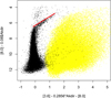 |
Fig. 1 CMD of AGB-like objects in a field of 1 square degree centered at l = 340° (black points) and YSOs in many directions (yellow points; Kuhn et al. 2021). Above the red line objects saturate the 3.6 μm- and/or the 8.0 μm-channel and their actual number might be higher. |
2 AGBs and YSOs, but mostly AGBs
In the earliest papers on the GLIMPSE database, Churchwell et al. (2009), Robitaille et al. (2008), two types of objects were distinguished: YSOs and AGBs. There may be other types of objects present as well, but as they are few, they are not included in this study. In the papers mentioned, we concluded that the ratio between the number of AGB stars and that of YSOs is on the order of 0.5.
We have drawn a different conclusion: YSOs are a very small minority. This follows from Fig. 1, which presents a color-magnitude diagram (CMD) of [3.6] – [8.0] versus [8.0], after a correction for the interstellar extinction. The 205 000 black points are objects from the GLIMPSE database, all located within one square degree centered on l = 340°, b = 0°. The red points are 120 000 YSO's identified by Kuhn et al. (2021) in 613 square degrees. The black and yellow points are well separated. Only a total of 218 GLIMPSE objects are in the yellow area. We conclude that the AGBs are by far the dominant population of the GLIMPSE database.
Another way to separate AGBs from YSOs has been given in Robitaille et al. (2008): objects with [4.5] < 7.8 are AGB stars and so are objects [4.5] > 7.8 when [8.0] – [24] < 2.5. Applying these criteria to the GH15 database, I found that 788 845 (84 percent) of the 933 818 entries are AGB stars, making them the dominant population in GLIMPSE by far.
Blum et al. (2006) carried out a comparable analysis of GLIMPSE objects in the Magellanic Clouds. They found oxygen-rich (O-rich) AGB stars, carbon-rich (C-rich) AGB stars, extreme AGB stars, red supergiants (RSGs), and galaxies. In our analysis, the extreme AGB stars and the RSGs are included in our AGB population; below, we show that C-rich AGB stars are not present in the inner Milky Way and galaxies might possibly be present, but we assume that their number is so small compared to the number of stars that the galaxies can be ignored.
The number of intrinsically red objects in the study by Robitaille et al. (2008) is much smaller than the number of AGB stars in our study. Robitaille et al. used two cut-offs ([4.5] – [8.0] > 0.76 and [8.0] < 9.68). We did not use these cutoffs and assumed instead that our larger number of objects consists of true AGB stars. Following the first published analyses of the GLIMPSE-database, we label the black points in Fig. 1 as "AGB stars." In the next section, we analyze the spectral energy distributions (SEDs) and confirm that this attribution is correct.
3 Stellar parameters mbol, AK, τCSE
3.1 The procedure
The spectral energy distribution (SED) of AGB stars is given by the magnitudes in the wavelength bands (J, H, K, [3.6], [4.5], [5.8], and [8.0]) modified by interstellar extinction, by emission by a circumstellar envelope (CSE) and by the difference in bolometric magnitude. Groenewegen (2006) has calculated the colors of a star of spectral type M with luminosity L = 3000 Lsun at the distance of the GC (m − M = 14.56) for CSEs for 18 different values of optical depth, τCSE. We added the interstellar extinction, AK as a free parameter for 80 different values of AK the extinction in the K-band at 2.2 μm For the extinction at other wavelengths we used the ratios by Messineo et al. (2005): (AJ,AH, AK, A3.6, A4.5, A5.8, A8.0) = (2.86, 1.66, 1.00, 0.3656, 0.2393, 0.1478, 0.08). The result is a matrix of 18*80 model SEDs. For a given star, we selected the model for which the SED has the same shape. We suppose that Δmj, j= 1 to 7, is the difference between the SED of the star and that of the model. Then the model is selected for which the values of Δmj are equal to their average as judged by the root mean square (rms) value of the seven differences. The chosen model then gives us values for two free parameters: AK and τCSE.
The difference between the mean value of Δmj and that of Groenewegens standard star is equal to the difference in bolo-metric magnitude of his standard star (10.55) and the selected star; we refer to this difference as dmag. The apparent bolometric magnitude of the stars is, thus, 10.55 + dmag. Figure 2 illustrates the rms analysis. The top diagram shows the magnitudes as a function of wavelength (see the caption of the figure). The bottom diagram shows the matrix of rms values (see the caption). The horizontal scale shows the 18 values of τCSE and the vertical scale AK from 0 to 4 in steps of 0.05; here the value of AK is securely determined, AK has little room for moving upward or downward. This is not the case in the horizontal direction: the contours are elongated. Therefore, the determination of τCSE is rather uncertain. Luckily, in almost all samples the same value of τ is obtained in many sources and we assume that the average of the τCSE values is meaningful.
3.2 Results
We analyzed the SED of more than 15 000 objects. They are all characterized by the SED of a M giant surrounded by a thin CSE. The SED analysis failed for almost all of the LPVs and the maser stars, as the CSEs are too thick. The results confirms that by far the most of the objects brighter than [8.0] = 11 are bona fide AGB stars.
3.2.1 Interstellar extinction, AK
The interstellar extinction was derived for about 25 000 GLIMPSE objects by comparing the SED, as observed, with theoretical models changed by interstellar absorption and circumstellar emission. This gave us for each object value of AK and of τCSE.
There is another, more direct determination of AK, proposed by Majewski et al. (2011). It is based on a narrow correlation between (J − H) and extinction that can be explained by elementary physics: the color at these long wavelengths can be approximated very well by the Rayleigh-Jeans approximation. Calling AKdir the extinction estimate from the Majewski-Zasowski method, we have

Figure 3 shows a narrow correlation between AKdir and AK, confirming that the two different ways to estimate AK are equivalent and we thus may skip the suffix Kdir.
In Paper II, we will discuss the spatial distribution of AK and, thus, the galactic distribution of interstellar dust.
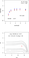 |
Fig. 2 Illustrations of the SED analysis. Top: wavelength shown horizontally and magnitude shown vertically. The black dots are the observations; they are partially visible because several coincide with red dots. Blue dots represent the chosen model i.e., the model with the SED that resembles best the SED of the observations. The chosen model plus dmag is in red. Diagram below: contours of the rms values. Vertically, AK and horizontally τCSE (the values 5, 10, and 15 correspond to τCSE = 0.005, 0.20, and 6.5). The red point is at the location of the minimum rms (0.223). Contour levels are 0.5, 0.7, and 1.0. |
3.2.2 Optical depth of the circumstellar envelope, τCSE
In his model, Groenewegen assumes emission by AlOx grains with known optical constants. Using his model we searched for circumstellar emission in about 15 000 AGB stars, sampling 1000 objects in 15 one square degree fields between −60° < l < 60°. In a fraction of 8%, the mean value of τCSE < 0.0002, in 19% it is between 0.0005 and 0.005, and in 73% between 0.010 and 0.94. Overall, CSEs are quite common, as expected of AGB stars, but always at modest optical depth.
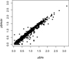 |
Fig. 3 Narrow correlation between values of the interstellar extinction derived in two different ways. |
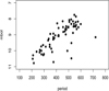 |
Fig. 4 mbol of the LPV stars discussed by Matsunaga et al. (2009) as derived by the least square method is plotted against the stellar period. |
3.2.3 Bolometric correction, dmag
To check our results of dmag we derived the apparent bolometric magnitude, mbo1 = 10.55 + dmag, using the SSTGC counterparts of long-period variables (LPVs) from Matsunaga et al. (2009). These are all close to the GC and have the same value of m − M = 14.5. For all LPVs we derived mbol = 10.55 + dmag. In Fig. 4, we give a plot of the period versus mbol. The correlation between m and period is apparent and agrees with the results on the LMC, apart from an offset of 4.5 magnitudes (Lebzelter et al. (2019)); the difference in distance between the LMC and the GC is 4.0 mag. For the remaining 0.5 mag (25% in luminosity), the lower metallicity in the MCs may provide the explanation. We still draw the conclusion that the least-squares determinations of dmag and of mbol are good enough for further discussion.
In each of the fields, the distribution of dmag is broad, as expected. The mean value of dmag varies with longitude (see Fig. 5). This mean value increases very steeply between l = ±10° and the GC. In Paper II, one of the main conclusions is that AGB stars with longitudes |l| < 10° from the GC are a population that is different from those at longitudes |l| > 10°. Figure 5 shows that there is systematic difference in mbo1 between the AGB stars near the GC and those farther out in the Galactic Disk.
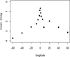 |
Fig. 5 Distribution of < dmag > as a function of longitude. Each point is based on dmag determinations in 1000 objects. |
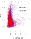 |
Fig. 6 Two CMDs, [K] − [8.0] versus [8.0], both corrected for interstellar extinction, of samples of objects in the directions l = 340° and l = 30°. |
4 Color-magnitude diagrams
A traditional way to start a statistical study of stellar populations is by constructing color-magnitude diagrams (CMDs). For a meaningful interpretation of CMDs of star samples in the Milky Way, we need to know the distances, μ = m − M, and this is not the case here. We do, however, argue that our CMDs still contain important information.
The GLIMPSE database contains stars residing deep into the Milky Way and the effects of foreground extinction by interstellar dust will be large. We determined AK by the procedure by Majewski et al. (2011), as discussed in the previous section.
Figure 6 is an example of two CMDs, where [8.0] − 0.08 • AK is the magnitude and [K] − AK − [8.0] + A8.0 is the color corrected for interstellar extinction. The figure contains 205 000 red-colored points in the 1 square degree field centered at (l, b) = (340°, 0°) and 174 000 blue points belonging to an equally large field at (l, b) = (30°, 0°). There is a cutoff at [8.0] < 4.0 due to detector saturation. The cutoff for [8.0] > 12.0 is caused by crowding of point sources and to interstellar extinction (see Sect. 5).
Figure 6 shows a surprisingly close coincidence of red and blue points: the two CMDs resemble each other closely although the lines of sight differ by 50°. The same conclusion follows by comparing the CMDs of all pairs from our sample of 31 one-square degree fields. These close resemblances convinced us that we are dealing with one and the same population of stars in all directions.
The large number of points in Fig. 6 hides a surprising property, which becomes visible in histograms: the distribution of the color (after correction for interstellar extinction) is remarkedly narrow. Figure 7 shows the histogram of [K] − AK − [8.0] + A8.0 in the field at l = 310°. The mean value is 0.08 and the rms-value with respect to this mean value is 0.02. In the other 31 fields the mean value varies systematically from 0.24 at l = 60°, to −0.13 at l = 0°, to 0.24 at l = 300° (see Fig. 8). The rms values are always small (≈0.02). The small but systematic change in the mean value is similar to the variation of mean value of dmag with longitude, as seen in Fig. 5. Both effects may plausibly be explained by a systematic decrease of metallicity from the direction toward the GC to that in the direction l = 60°.
This very narrow distribution of colors in all directions (over a range of 120° in longitude; i.e., the full GLIMPSE database) is impressive: the stars have all the same color and a considerable range in apparent magnitude. Girardi et al. (2000) demonstrated theoretically that AGB stars increase rapidly their luminosity by as much of five absolute magnitudes or by a factor of 100 in luminosity, whereas the surface temperature Teff increases by only 25%. This conclusion confirms what has been said in the previous section, that practically all objects in GLIMPSE are AGB stars; at least, those brighter than [8.0] = 12.
In contrast to the colors, the luminosities of AGB stars have a broad distribution. This appears by adding to the CMDs objects that are known to be AGB stars: LPVs and SiO and OH masers. From the GLIMPSE database, we identified 1340 LPV stars from Matsunaga et al. (2009), 180 SiO masers from Deguchi et al. (2004), and 54 OH/IR masers from Sjouwerman et al. (1998). The identification was based on a coincidence in position within 2 arcsec. All objects in these three surveys are at the distance of the GC.
Figure 9 shows the results. The colored samples join the GLIMPSE objects around the magnitude [8.0] = 7 and then turn to the right in the direction of cooler (redder) colors. Masers and LPVs have a redder color and their luminosity is higher than those of the other AGB stars; thus, their diameter should be larger as well. The fact that the distribution of the LPV and maser samples join the GLIMPSE objects confirms that they are extreme AGB stars.
In Fig. 9, the red points have a smaller color and a smaller magnitude than the blue points. The blue points are supposed to be stars of higher mass than the red points. Thus, in the very end, stars of higher mass have somewhat higher luminosities and somewhat redder colors, while the radii of the blue objects will be larger than those of the red objects.
All these arguments lead us to the conclusion that the CMDs in this paper illustrate the evolution of AGB stars; the vertical structure indicates the increase of the luminosity of AGB stars and shows how they end as LPV or maser star. In Sect. 5, we give additional information on how fast the AGB stars increase in luminosity.
The luminosity distribution of AGB stars is very broad and from a single CMD, we cannot reliably extract the stellar distances. By combining CMDs taken in different longitude directions we see (Fig. 10) that the total number of stars increases strongly in the direction of the GC. There is a rough symmetry with respect to l = 0° indicating that the stars we study form a kind of disk around the GC. This will be elaborated on in Paper II.
A final comment concerns the fact that there are two kinds of AGB stars: O- and C-rich AGB stars. In the inner Milky Way, (|l| ≤ 60°, the C-rich AGBs are a small minority, compared to the O-rich stars (Blanco & Terndrup 1989, Lewis et al. 2020). A small number of known C-rich AGB stars in the inner Milky Way might contradict this conclusion, but Matsunaga et al. (2017) showed that these stars are all members of a binary system with mass exchange; thus, these stars not the AGB stars discussed in the current paper. Another indication is the absence of C-rich AGB stars in a study of near-infrared (NIR) spectra of 45 objects by Uttenthaler et al. (2015). Finally, Cioni & Habing (2003) noticed that in the Large Magellanic Cloud, C-rich AGB stars are separated from the oxygen rich stars by the criterion J – K < 1.4 (oxygen rich stars) and J – K > 1.4 (carbon-rich stars). Figure 5 shows the distribution of the (J – K) color before and after correction for extinction, all in an area of 1 square degree in the direction (l, b) = (5°, 0°). The extinction of this sample residing close to the GC is very high and, thus, the correction for extinction of the J – K-values is also high. Although a minority of stars have a corrected value of J – K larger than 1.4, we ignored this small number in comparison to the large number of sources with J – K < 1.4. Overall, all the AGB stars in the GLIMPSE-database are O-rich.
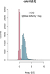 |
Fig. 7 Distribution of color Kmag − [8.0] of GLIMPSE objects in a 1 square degree field in the direction l = 310°. Light blue: Before correction for interstellar extinction. Pink: After correction. The blue points have been shifted artificially by +1.0 mag. |
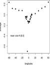 |
Fig. 8 Mean color of stars in Fig. 7 after correction for interstellar extinction and as a function of galactic longitude. |
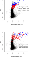 |
Fig. 9 CMD in the direction l = 10° with (upper diagram) the addition of LPVs (red: per < 500 d, blue: per > 500 d) and (lower diagram) maser stars (red: SiO masers, blue: OH masers). |
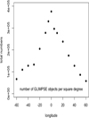 |
Fig. 10 Number of GLIMPSE objects in fields of 1 square degree as as function of galactic longitude. Galactic latitude is 0°. |
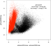 |
Fig. 11 Histograms of the J-magnitude minus the K-magnitude before (black points) and after correction (red points) for interstellar extinction. All objects taken from an area of 1 square degree at l = 5°. |
5 Counting the stars
We counted the number of stars per square degree in 31 directions along the galactic plane and in magnitude intervals of 0.5 magnitude from [8.0] = 5 to 12. The result is a matrix Nml; here m is the apparent magnitude and l the longitude. This matrix is discussed in this paper as a function of m for constant l. In Paper II, we discuss Nml as a function of l for constant m. Before proceeding further, it is necessary to consider the completeness of the data.
5.1 Incompleteness and nondetection of sources with [8.0] ≥ 11: seeing the AGB disk end
The sensitivity limit of GLIMPSE at 8 μm is magnitude 13.5 according to Churchwell et al. (2009). This is true only for the detection of a single, well-isolated star without variable continuous background emission. In this paper, areas of high density are studied and problems arise due to confusion of sources and to a variable background. As an example, GLIMPSE maps in (l, b) frequently show empty areas at faint magnitudes (e.g., at magnitude [8.0] ≥ 11), as shown in Figs. 12 and 13. The plots also show that the size of these open areas is smaller the farther away they are located from the GC.
Incompleteness is a threat for any statistical study but some information on fainter stars remains. The two (l, b) plots in Fig. 13 show stars in the same area of one square degree with (above) stars with 11 .0 < [8.0] < 12.0 and (below) with 12.0 < [8.0] < 13.0. While empty areas are clearly seen, there are other and significant areas that show that the stellar density decreases drastically between magnitudes 11.00/11.99 and 12.00/12.99. There are much fewer stars fainter than magnitude 12.0 because they disappear from sight; we reached the faint end of the distribution in the Milky Way of O-rich AGB stars.
The decrease in numbers of AGB stars for [8.0] > 12.0 is not a surprise. From IRAS observations and from maser searches we know that there are few O-rich AGB stars in the anti-center direction (Habing et al. 1985, Blommaert et al. 1993). This suggests that in the GC-direction, we expect to find no similar AGB stars beyond 2 • RGC = 16.4 kpc, corresponding to m − M = 16. The counts continue to rise until [8.0] = 11. The faintest stars at that distance will have a bolometric magnitude Mbol = −2.5 and this is an acceptable lower limit for the bolometric magnitude of an early AGB star.
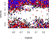 |
Fig. 12 (l, b) map centered on the GC and containing GLIMPSE objects of magnitudes 10.75 ± 0.25 (black), 11.25 ± 0.25 (red) and 11.75 + 0.25 (blue). |
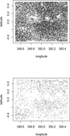 |
Fig. 13 (l, b) plots of a field of 1 square degree centered on (l = 350°, b = 0°) for stars with 11.0 < [8.0] < 11.99 (top) and 12.0 < [8.0] < 12.99 (bottom). The empty areas are conspicuous and large in both diagrams. Yet there remains a significant area without extinction effects and in these areas the number density in the fainter diagram is considerably lower. |
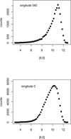 |
Fig. 14 Counts of stars in directions l = 340° and 0° within one square degree and a within a width of 0.5 magnitude. |
5.2 Nml: Counting the stars as a function of magnitude [8.0] at constant longitude; exponential distributions
The most interesting part of Nml lies between [8.0] = 5 and 11. For [8.0] > 11.0, the numbers decrease sharply for reasons discussed above. At the bright end, ([8.0] ≤ 5.0), there is a shortage of sources for different reasons: the detectors might have saturated and the one square degree field does not contain all nearby stars at that longitude.
We first consider the counts, Nml, in the directions l = 340° and l = 0° in Fig. 14. The numbers increase very fast to fainter magnitudes; this is the same in all directions along the plane of the Milky Way. Figure 15 shows the same two diagrams but now after expressing the counts in log10. The logarithm of the counts in the l = 340° diagram contains a linear part between magnitudes [8.0] = 5 and 11. In the l = 0°-diagram, there is no indication of a linear part; rather, the points form a curve.
The slope of the linear part, present in all diagrams for |l| > 10°, is always the same: between 0.33 and 0.35. For |l| < 10°, the counts show a curvature. Both conclusions will be explained below.
The linearity of log10(Nml) is not a new discovery. Figure 12 in Churchwell et al. (2009) shows lines with the same slope in the log(N) distribution. However, that paper does not discuss the next question: why are many magnitude distributions exponential?
5.3 Why are many magnitude distributions exponential?
Quite generally, we can write the number, Nml, in the direction, l, as an integral along the line of sight as

Here, μ = m − M is the distance modulus and ρ is the stellar density; σ is the area of 1 square degree at the distance μ = m − M over which the stars are counted, σ = r2 • Ω. Ω is the solid angle of 1 square degree. Ψ is the distribution of absolute bolometric magnitudes.
The observations showed that in the outer disk Nml is an exponential function in m. The derivative of an exponential function is another exponential function: integration nor differentiation creates or destroys an exponential function. Thus, the integrand ρ(μ) • σ(μ) · Ψ must contain an exponential function. Neither ρ(μ) nor σ(μ) are expected to be exponential and the luminosity function Ψ(M) is most likely the culprit. Support for this conclusion can be found in calculations of the increase in time of the luminosity of AGB stars.
Figure 16 shows the increase in luminosity during the AGB phase of a star of 2Msun; the diagrams for stars of other mass are similar. Because log L ∝ t it follows that L(t) = L0 10a•t. Supposing that n0 stars enter the AGB with luminosity, L0 and then increase in luminosity continously; at each point in time, we suppose that n(t) • dL/dt = n0 • (dL/dt)0. Thus, at a luminosity, L, their number n is given by n • L = n0 • L0.
We write Ψ(L) = n0L0/L. Thus, we obtain

Inside the integral the product L/r2 = 100.4(4.84−m) is a constant, because m is constant in the integration. The deeper reason is this is: traveling along a line of sight at a fixed value of the a2pparent magnitude, m, the luminosity of stars will increase as r2 and, thus, their number, n, decreases by a factor 1/r2. At the same time, the area over which we collect stars becomes larger by a factor r2; the product L/r2 is a constant. We arrive at

where A = n0 • L0 • Ω • 10−0.4•4.84.
The integral is a function of m because the path of integration, depends on m. At longitudes |l| > 10°, in the outer disk, the observations show that log 10(Nml) is a linear function of m with a slope of the line between 0.33 and 0.36. Consequently, in the outer disk the integral depends on apparent magnitude as m ∝ 10(0.40−0.36)•m and this is confirmed in the following subsection.
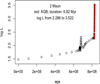 |
Fig. 16 Calculations of the luminosity of a star of 2 Msun by Girardi et al. (2000). In red the luminosity during the AGB phase. |
5.4 A smeared out map of the distribution of AGB stars in the plane of the Milky Way
We introduce a new matrix, Rml = Nml • 10−0.4m/A, or

Here, Rml is the integral of ρ over the distance range μ = m − M0 and μ = m − M1 and thus Rml represents a smeared out version of ρ. In the outer disk, in the longitude range of (|l| ≥ 10°, Rml ∝ 10−0.06 and, thus, Nml ∝ 100.4−0.06. This explains the slope of the linear parts in the graphs of m versus Nml in Fig. 14. Ultimately, this is a consistency check for the statement that Ψ = n0L0/L.
Contour diagrams of the function Rml as a function of l and m are shown in Fig. 17. In the top diagram, the longitude steps are 10° from l = −60° to = +60°. The bottom diagram is in longitude steps of only one degree.
The upper diagram shows activity only for 10° > l > −10° ; the GLIMPSE AGB stars are strongly concentrated toward the GC. The lower diagram has a higher angular resolution (1 °) and shows that the activity is even more limited in extent, 1° > l > −1 °. The diagrams contain two maxima: one of stars at bright magnitude ([8.0] = 4) belonging to the Nuclear Stellar Disk and the other at ([8.0] = 8) representing the inner part of the Galactic Bulge. The magnitude 4 of stars in the Nuclear Stellar Disk (i.e., at a distance μ = 14.56) corresponds to absolute magnitudes M = −10.5 or L = 1.4 • 106 Lsun. This is exceptionally high for an AGB star.
The two diagrams in Fig. 17 show symmetry with respect to the line at l = 0°; this suggests an axial distribution around the GC. The two diagrams in Fig. 17 will be the basis for a further discussion in Paper II of the distribution of the AGB stars in the inner Milky Way.
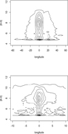 |
Fig. 17 Contour diagrams of the function Rml, the smeared out distribution of the AGB stars in the Milky Way. Horizontally the galactic longitude, vertically the apparent magnitude at 8.0 μm. The top figure shows that the strong features are limited to −5.0 < l < +5.0. The lower figure shows that the strong features are even narrower and limited to −1.0 < l < +1.0. |
6 Conclusions
At 8.0 μm, the Milky Way is transparent. The GLIMPSE database contains all O-rich AGB stars in the Milky Way between longitudes −60° and +60°.
Objects in the GLIMPSE database with [8.0] ≤ 11.0 are characterized by a spectral energy distribution (SED) that is well described by those of late M giants surrounded by a thin dusty CSE and seen through much (foreground) interstellar dust. The objects must be AGB stars, although a small fraction of RSGs and YSOs is also present; this fraction is so small that we have ignored them in the discussions;
All CMDs display a vertical track of stars between [8.0] = 11 and 6.5 with a mean color of 0 mag and a rms of 0.01. The small spread of the color is explained by the intrinsic nature of AGB stars;
Maser stars and LPVs residing near the Galactic Centre, following the identification of their GLIMPSE counterparts, have bright magnitudes and appear in the CMDs as a continuation of the vertical track discussed before. They have thick CSEs, which confirms once again that LPVs and maser stars are AGB stars in the last evolutionary phase, losing mass at a high rate;
We interpret the CMDs as a demonstration of the evolution of AGB stars. Starting at low luminosities, they increase rapidly in luminosity, but keep their color until they reach [8.0] ≈ 7; after this point, the stars start loosing mass very rapidly;
For |l| > 10°, the number of stars increases exponentially with magnitude (e.g., at 8.0 μm). This is explained by the exponential increase in time of the luminosity of AGB stars;
Between [8.0] = 11 and [8.0] = 12 the number of AGB stars per square degree decreases rapidly when the end of the disk of AGB stars is approached and it is not an instrumental effect;
From the counts in longitude and magnitude, a matrix Rml can be derived to represent a smeared-out distribution of AGB stars in the inner Milky Way. The inner Galactic Bulge and the Nuclear Stellar Disk are prominent features.
The GLIMPSE database contains millions of AGB-stars. The stellar color after correction for interstellar extinction is always the same. The number of stars increases exponentially with apparent magnitude because of the exponential increase of the stellar luminosity with time.
References
- Baade, W. 1975, Evolution of Stars and Galaxies, ed. C. Payne-Gaposchkin (MIT Press) [Google Scholar]
- Blanco, V. M., & Terndrup, D. M. 1989, AJ, 98, 843 [Google Scholar]
- Blommaert, J. A. D. L., van der Veen, W. E. C. J., & Habing, H. J. 1993, A&A, 267, 39 [NASA ADS] [Google Scholar]
- Blum, R. D., Mould, J. R., Olsen, K. A., et al. 2006, AJ, 132, 2034 [NASA ADS] [CrossRef] [Google Scholar]
- Churchwell, E., Babler, B. L., Meade, M. R., et al. 2009, PASP, 121, 213 [Google Scholar]
- Cioni, M. R. L., & Habing, H. J. 2003, A&A, 402, 133 [NASA ADS] [CrossRef] [EDP Sciences] [Google Scholar]
- Deguchi, S., Imai, H., Fujii, T., et al. 2004, PASJ, 56, 261 [NASA ADS] [Google Scholar]
- Girardi, L., Bressan, A., Bertelli, G., & Chiosi, C. 2000, A&AS, 141, 371 [NASA ADS] [Google Scholar]
- Groenewegen, M. 2006, A&A, 448, 181 [NASA ADS] [CrossRef] [EDP Sciences] [Google Scholar]
- Gutermuth, R. A., & Heyer, M. 2015, ApJ, 149, 64 [Google Scholar]
- Habing, H. J., Olnon, F. M., Chester, T., Gillett, F., & Rowan-Robinson, M. 1985, A&AL, 152, L1 [Google Scholar]
- Kobulnicky, H. A., Babler, B. L., Alexander, M. J., et al. 2013, ApJS, 207, 9 [Google Scholar]
- Kuhn, M. A., de Souza, R. S., Krone-Martins, A., et al. 2021, ApJS, 254, 33 [NASA ADS] [CrossRef] [Google Scholar]
- Lebzelter, T., Trabucchi, M., Mowlavi, N., et al. 2019, A&A, 631, A24 [NASA ADS] [CrossRef] [EDP Sciences] [Google Scholar]
- Lewis, M. O., Pihlström, Y. M., Sjouwerman, L. O., Stroh, M. C., & Morris, M. R. 2020, ApJ, 892, 52 [NASA ADS] [CrossRef] [Google Scholar]
- Majewski, S. R., Zasowski, G., & Nidever, D. L. 2011, ApJ, 739, 25 [Google Scholar]
- Matsunaga, N., Kawadu, T., Nishiyama, S., et al. 2009, MNRAS, 399, 1709 [NASA ADS] [CrossRef] [Google Scholar]
- Matsunaga, N., Menzies, J. W., Feast, M. W., et al. 2017, MNRAS, 469, 4949 [NASA ADS] [CrossRef] [Google Scholar]
- Messineo, M., Habing, H. J., Menten, K. M., et al. 2005, A&A, 435, 575 [NASA ADS] [CrossRef] [EDP Sciences] [Google Scholar]
- Ramírez, S. V., Arendt, R. G., Sellgren, K., et al. 2008, ApJS, 175, 147 [Google Scholar]
- Reid, M. J., Menten, K. M., Brunthaler, A., et al. 2019, ApJ, 885, 131 [Google Scholar]
- Robitaille, T. P., Meade, M. R., Babler, B. L., et al. 2008, AJ, 136, 2413 [NASA ADS] [CrossRef] [Google Scholar]
- Robitaille, T. P., Churchwell, E., Benjamin, R. A., et al. 2012, A&A, 545, A39 [NASA ADS] [CrossRef] [EDP Sciences] [Google Scholar]
- Sjouwerman, L. O., van Langevelde, H. J., Winnberg, A., & Habing, H. 1998, A&AS, 128, 35 [Google Scholar]
- Skrutskie, M. F., Cutri, R. M., Stiening, R., et al. 2006, AJ, 131, 1163 [NASA ADS] [CrossRef] [Google Scholar]
- Trumpler, R. 1930, Lick Obs. Bull., XIV, 154 [Google Scholar]
- Uttenthaler, S., Blommaert, J. A. D. L., Wood, P. R., et al. 2015, MNRAS, 451, 1750 [Google Scholar]
All Figures
|
Fig. 1 CMD of AGB-like objects in a field of 1 square degree centered at l = 340° (black points) and YSOs in many directions (yellow points; Kuhn et al. 2021). Above the red line objects saturate the 3.6 μm- and/or the 8.0 μm-channel and their actual number might be higher. |
| In the text | |
|
Fig. 2 Illustrations of the SED analysis. Top: wavelength shown horizontally and magnitude shown vertically. The black dots are the observations; they are partially visible because several coincide with red dots. Blue dots represent the chosen model i.e., the model with the SED that resembles best the SED of the observations. The chosen model plus dmag is in red. Diagram below: contours of the rms values. Vertically, AK and horizontally τCSE (the values 5, 10, and 15 correspond to τCSE = 0.005, 0.20, and 6.5). The red point is at the location of the minimum rms (0.223). Contour levels are 0.5, 0.7, and 1.0. |
| In the text | |
|
Fig. 3 Narrow correlation between values of the interstellar extinction derived in two different ways. |
| In the text | |
|
Fig. 4 mbol of the LPV stars discussed by Matsunaga et al. (2009) as derived by the least square method is plotted against the stellar period. |
| In the text | |
|
Fig. 5 Distribution of < dmag > as a function of longitude. Each point is based on dmag determinations in 1000 objects. |
| In the text | |
|
Fig. 6 Two CMDs, [K] − [8.0] versus [8.0], both corrected for interstellar extinction, of samples of objects in the directions l = 340° and l = 30°. |
| In the text | |
|
Fig. 7 Distribution of color Kmag − [8.0] of GLIMPSE objects in a 1 square degree field in the direction l = 310°. Light blue: Before correction for interstellar extinction. Pink: After correction. The blue points have been shifted artificially by +1.0 mag. |
| In the text | |
|
Fig. 8 Mean color of stars in Fig. 7 after correction for interstellar extinction and as a function of galactic longitude. |
| In the text | |
|
Fig. 9 CMD in the direction l = 10° with (upper diagram) the addition of LPVs (red: per < 500 d, blue: per > 500 d) and (lower diagram) maser stars (red: SiO masers, blue: OH masers). |
| In the text | |
|
Fig. 10 Number of GLIMPSE objects in fields of 1 square degree as as function of galactic longitude. Galactic latitude is 0°. |
| In the text | |
|
Fig. 11 Histograms of the J-magnitude minus the K-magnitude before (black points) and after correction (red points) for interstellar extinction. All objects taken from an area of 1 square degree at l = 5°. |
| In the text | |
|
Fig. 12 (l, b) map centered on the GC and containing GLIMPSE objects of magnitudes 10.75 ± 0.25 (black), 11.25 ± 0.25 (red) and 11.75 + 0.25 (blue). |
| In the text | |
|
Fig. 13 (l, b) plots of a field of 1 square degree centered on (l = 350°, b = 0°) for stars with 11.0 < [8.0] < 11.99 (top) and 12.0 < [8.0] < 12.99 (bottom). The empty areas are conspicuous and large in both diagrams. Yet there remains a significant area without extinction effects and in these areas the number density in the fainter diagram is considerably lower. |
| In the text | |
|
Fig. 14 Counts of stars in directions l = 340° and 0° within one square degree and a within a width of 0.5 magnitude. |
| In the text | |
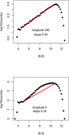 |
Fig. 15 log10 of the counts in Fig. 13. Linear part in red. |
| In the text | |
|
Fig. 16 Calculations of the luminosity of a star of 2 Msun by Girardi et al. (2000). In red the luminosity during the AGB phase. |
| In the text | |
|
Fig. 17 Contour diagrams of the function Rml, the smeared out distribution of the AGB stars in the Milky Way. Horizontally the galactic longitude, vertically the apparent magnitude at 8.0 μm. The top figure shows that the strong features are limited to −5.0 < l < +5.0. The lower figure shows that the strong features are even narrower and limited to −1.0 < l < +1.0. |
| In the text | |
Current usage metrics show cumulative count of Article Views (full-text article views including HTML views, PDF and ePub downloads, according to the available data) and Abstracts Views on Vision4Press platform.
Data correspond to usage on the plateform after 2015. The current usage metrics is available 48-96 hours after online publication and is updated daily on week days.
Initial download of the metrics may take a while.