


| Issue |
A&A
Volume 711, July 2026
|
|
|---|---|---|
| Article Number | A224 | |
| Number of page(s) | 14 | |
| Section | Astrophysical processes | |
| DOI | https://doi.org/10.1051/0004-6361/202453642 | |
| Published online | 20 July 2026 | |
Modeling accretion columns in accretion-powered pulsars
I. Accretion column emission and geometry
1
Dr. Karl Remeis-Observatory & ECAP, University of Erlangen-Nuremberg, Sternwartstr. 7, 96049 Bamberg, Germany
2
NASA Goddard Space Flight Center, Astrophysics Science Division, Greenbelt, MD 20771, USA
3
CRESST, Department of Astronomy, University of Maryland, College Park, MD 20742, USA
4
International Space Science Institute, Hallerstrasse 6, 3012 Bern, Switzerland
5
Physikalisches Institut, University of Bern, Sidlerstrasse 5, 3012 Bern, Switzerland
6
ISDC, Department of Astronomy, University of Geneva, Chemin d’Ecogia 16, 1290 Versoix, Switzerland
7
INAF, Osservatorio Astronomico di Brera, Via E. Bianchi 46, I-23807 Merate, Italy
8
Sternberg Astronomical Institute, M. V. Lomonosov Moscow State University, Universitetskij pr., 13 Moscow 119992, Russia
9
Leibniz-Institut für Astrophysik Potsdam (AIP), An der Sternwarte 16, 14482 Potsdam, Germany
10
Space Science Division, Naval Research Laboratory, Washington, DC 20375-5352, USA
11
Department of Physics & Astronomy, George Mason University, Fairfax, VA 22030-4444, USA
12
CRESST and Center for Space Sciences and Technology, UMBC, Baltimore, MD 21250, USA
13
European Space Astronomy Center (ESA/ESAC), Science Operations Department, Villanueva de la Cañada, 28691, Madrid, Spain
14
Astronomy and Astrophysics Dept., University of California San Diego, La Jolla, CA 92075, USA
15
Boston Fusion Corp., 70 Westview, Suite 100 Lexington, MA 02421, USA
16
Institut für Astronomie und Astrophysik, Universität Tübingen, Sand 1, 72076 Tübingen, Germany
★ Corresponding authors: This email address is being protected from spambots. You need JavaScript enabled to view it.
; This email address is being protected from spambots. You need JavaScript enabled to view it.
Received:
31
December
2024
Accepted:
9
April
2026
Abstract
Context. Accretion-powered X-ray pulsars show complex spectral and timing behavior that reflects the extreme conditions near the neutron star. Modeling these observables remains challenging, particularly at high mass-accretion rates, Ṁ ≳ 1017 g s−1, where the extended accretion column plays a role in shaping anisotropic emission seen by a remote observer.
Aims. Here, we present a modular framework that links radiation processes inside the column to the emission observed at infinity. The framework combines existing models for continuum and cyclotron resonant scattering feature (CRSF) formation in sidewall column emission with ray tracing, thereby bridging the gap between the rest-frame emission and the observable flux.
Methods. We model the radiation from the accretion column using continuum emission from the column walls, calculated in the regime of saturated Comptonization in the presence of a radiation-dominated shock. This emission then passes through a thin outer layer with a fast-moving bulk flow, where CRSFs, derived from Monte Carlo simulations, are imprinted. Finally, a geometry-independent ray-tracing code accounts for light bending in the Schwarzschild metric, incorporating the shape and location of the emitting regions and neutron star rotation to compute the observed phase- and energy-dependent flux.
Results. We present the height-dependent anisotropic emission in the column rest frame. For the chosen model, approximately 70% of the radiation is emitted within 1 km of the base of the column, predominantly at large angles to the magnetic field. Relativistic boosting in the bulk flow affects the appearance of CRSFs in the spectra, leading to a strong dependence of the line locations on the angle relative to the magnetic field.
Conclusions. The proposed theoretical framework allows a straightforward combination of internal emission models with ray tracing to study the observed flux. Here, we focus on the joint treatment of the two-dimensional column structure and CRSF formation in the neutron star rest frame. The observed phase and spectral variations of the flux are highly sensitive to the location of the emitting regions and the observer’s viewing angle, which is explored in an accompanying paper.
Key words: radiative transfer / relativistic processes / methods: numerical / stars: neutron / X-rays: binaries
Deceased 6 March 2025.
Deceased 17 June 2025.
© The Authors 2026
 Open Access article, published by EDP Sciences, under the terms of the Creative Commons Attribution License (https://creativecommons.org/licenses/by/4.0), which permits unrestricted use, distribution, and reproduction in any medium, provided the original work is properly cited.
This article is published in open access under the Subscribe to Open model. This email address is being protected from spambots. You need JavaScript enabled to view it. to support open access publication.
1. Introduction
Accretion-powered X-ray pulsars are neutron stars with strong magnetic fields, found in binary systems where they accrete matter from a companion star. This scenario is most commonly observed in high-mass X-ray binaries, which host relatively young (∼105–106 yr), slowly rotating neutron stars with spin periods of ∼1–1000 s and magnetic field strengths of ∼1012–1013 G. The extended magnetosphere of a neutron star stops the accretion flow thousands of kilometers above the surface and channels the infalling plasma onto the magnetic poles, forming localized emission regions where the flow decelerates. If the spin and magnetic axes are misaligned, a remote observer can see periodic changes in the flux as the emission regions rotate through the line of sight (Lamb et al. 1973). For reviews of these systems, see, for example, Caballero & Wilms (2012) and Mushtukov & Tsygankov (2023).
During accretion onto a neutron star surface, the kinetic energy of the plasma is converted into radiation. At high mass-accretion rates relevant for this work, Ṁ ≳ 1017 g s−1, the resulting radiation pressure is sufficiently strong to influence the dynamics of the infalling flow, leading to a significant radiative deceleration of the plasma (Davidson 1973; Basko & Sunyaev 1976). Several analytical and numerical studies of two-dimensional radiation hydrodynamics have demonstrated that the radiation-dominated shock takes a mound-like shape, with its characteristic height of hundreds meters to several kilometers away from the neutron star surface (see, e.g., Davidson 1973; Wang & Frank 1981; Klein & Arons 1989; Klein et al. 1996; Postnov et al. 2015; Gornostaev 2021; Zhang et al. 2022; Markozov et al. 2024; Gornostaev 2025). The velocity of the flow in the accretion mound is greatly reduced, and final deceleration can occur via charged particle collisions (Basko & Sunyaev 1976; Wang & Frank 1981). These models consistently show that at the edge of the accretion column the free-fall region extends almost down to the neutron star surface (Klein 1997). The spectral formation in the shock and the accretion mound is primarily driven by the bulk and thermal Comptonization of bremsstruhlung and cyclotron emission (Arons et al. 1987; Becker & Wolff 2007).
In a strong magnetic field of ∼1012 G, the electron motion perpendicular to the field is quantized into Landau levels, with energy separations that fall in the X-ray range (e.g., Canuto et al. 1971; Mészáros 1992). This introduces resonances to radiative processes, such as photon emission and Compton scattering. The latter leads to the formation of cyclotron resonant scattering features (CRSFs) in the form of broad absorption features, also known as cyclotron lines. These features typically vary with pulse phase in energy, depth, and width (see Staubert et al. 2019, for a comprehensive review). These variations can be attributed to the strong angular dependence of the cyclotron scattering cross section, relativistic aberration due to the high velocity of the free-fall (∼60% of the speed of light), and the contribution from several spectral-forming regions. In some sources, the observed CRSF energy varies with the source luminosity, L, typically showing a positive correlation at lower luminosity (L ≲ 1037 erg s−1) and a negative correlation at higher luminosity (e.g., Staubert et al. 2007; Tsygankov et al. 2010; Becker et al. 2012; Poutanen et al. 2013; Lutovinov et al. 2015, and references therein). These variations are generally interpreted as changes in the structure of the emission region or characteristics of the flow (e.g., velocity profile) interacting with photons in the channel (Becker et al. 2012; Mushtukov et al. 2015; Loudas et al. 2024).
One of the most vexing questions is which region is primarily responsible for the formation of observed CRSFs in the high-Ṁ regime. The accretion column emits mainly from the side walls (with the emission pattern typically described as a fan beam), with the optically thick accretion mound serving as a primary source of radiation (see, e.g., Burnard et al. 1991; Klein et al. 1996; Postnov et al. 2015). It is often assumed that the CRSF-forming region is associated with the radiation-dominated shock, so that variations in CRSF energy reflect changes in the characteristic height of the shock (Becker et al. 2012; Loudas et al. 2024). However, the radiation energy density increases toward the base of the accretion channel, below the shock (e.g., Zhang et al. 2023; Gornostaev 2025), and several studies indicate that most of the radiation escapes through the sidewalls of the accretion column near the neutron star surface (Postnov et al. 2015; Gornostaev 2021). In this scenario, the dynamic structure of the column, and in particular the outer free-fall layer extending down along the sides of the accretion mound, can affect line formation. Only a few simulations have addressed this problem while accounting for the two-dimensional channel structure, and these were limited to intermediate mass-accretion rates (Ṁ ≈ 1016–1017 g s−1), where photon–flow interactions are weaker, producing a pronounced CRSF in the spectrum of the radiation in the neutron star rest frame (Rebetzky et al. 1989, Markozov et al. 2024, see also also the preprint by Fotiadis et al. 2026 for a similar regime with a one-dimensional velocity distribution in the channel). An alternative scenario attributes the formation of CRSFs to the neutron star surface, either heated by collisional stopping (in the outer rim of the column; Wang & Frank 1981) or illuminated by the column emission (Poutanen et al. 2013; Kylafis et al. 2021).
Distinguishing between these scenarios requires one to compare model predictions with observations. For accretion-powered X-ray pulsars, strong phase variability and complex spectral energy distributions provide additional insights into the source behavior. Modern X-ray missions and recently proposed analysis tools (e.g., Ferrigno et al. 2023) have greatly expanded the observational basis. However, on the modeling side, the phase and energy domains are often treated separately. A consistent description requires one to model the observed flux of angle- and energy-dependent radiation emitted from regions with specified geometry and location, and project it onto the observer’s plane. This is challenging due to the complexity of spectral formation in the strongly magnetized plasma of the accretion column, often leading to neglect of one or more dimensions (e.g., photon energy, angle, or a height distribution of the emission). Moreover, most emission models address only spectral formation in the plasma or neutron star rest frame, omitting general relativistic effects and contributions from multiple emission regions, which can significantly influence the observed flux. In this work, we integrate these aspects within a unified modeling framework.
A formalism to account for gravitational light bending and the Doppler effect in modeling the observed emission from a slowly rotating neutron star was proposed by Pechenick et al. (1983) and is widely adopted in the field of accretion-powered X-ray pulsars. Modeling the observed flux necessitates calculating the trajectories of emitted photons in curved space-time, which quickly becomes computationally expensive. Several analytic solutions have been proposed (e.g., Beloborodov 2002; Poutanen & Beloborodov 2006; Poutanen 2020, and references therein) and successfully applied to obtain pulse profiles from emission regions, such as hot spots on the neutron star surface (e.g., Beloborodov 2002; Poutanen & Beloborodov 2006; Cappallo et al. 2017; Markozov & Mushtukov 2024), or extended cylindrical and conical accretion columns (Ferrigno et al. 2011; Markozov & Mushtukov 2024). The models have evolved from point-like sources on the neutron star surface to extended emission regions, which can also be placed asymmetrically, and thus resemble offset dipole geometries. However, most models still rely on the assumption of azimuthal symmetry of the emission region, which simplifies the modeling.
We present a flexible ray-tracing code for the Schwarzschild metric that enables general modeling of the observed flux. Originally developed by Falkner (2013, 2018), it has been applied with phenomenological emission profiles to fit pulse profiles of 4U 1626−67 (Iwakiri et al. 2019), combined with a hotspot emission model to describe the low-luminosity state of GX 304−1 (Sokolova-Lapa 2023), and used as the basis for a simpler, lightweight model for EXO 2030+375 (Thalhammer et al. 2024). Unlike most earlier approaches, the code implements full numerical ray tracing in the Schwarzschild metric and, in principle, imposes no intrinsic restrictions or symmetry assumptions on the emission region.
Here, we introduce a framework that combines physical models for emission in the falling plasma and neutron star rest frames with a ray-tracing code. This setup enables us to study the phase and energy variability of the sidewall column emission and observability of CRSFs. We provide a detailed description of the individual emission components and their integration in Sect. 2. Section 3 presents the resulting emission from the accretion column in the neutron star rest frame and provides an example of observed phase-dependent flux. Section 4 summarizes the modeling approach and discusses key model-specific results and limitations. A more detailed study of energy- and phase-dependent emission for different column locations and viewing angles is presented in an accompanying paper (Falkner et al. 2026, Paper II).
2. Accretion column and emission model
We considered accretion onto a strongly magnetized, B ∼ 1012 G, and slowly rotating neutron star, P > 1 s in the radiation-dominated regime described above, Ṁ ∼ 1017 g s−1, where an extended accretion column forms. We assumed a cylindrical column, with radiation emerging from its sidewalls in a “fan beam”. In order to obtain a quasi-realistic energy-dependent emission profiles, we combined two different models for emission: the continuum obtained in the regime of saturated Comptonization from a two-dimensional hydrodynamic column structure by Postnov et al. (2015) (Sect. 2.1), and the cyclotron scattering model by Schwarm et al. (2017a,b) (Sect. 2.2). As is illustrated in Fig. 1, we divided the column itself into two parts: a dense inner volume that is optically thick (Thomson optical depth τ ≳ 1) and in which the continuum emission is formed, and a geometrically thin layer that surrounds this region. While optically thin to the continuum radiation, this layer is still optically thick at energies near the cyclotron resonances, such that CRSFs are imprinted onto the continuum. We then transformed the emission into the neutron star rest frame (Sect. 2.3) and projected it onto the observer’s plane, accounting for light bending and gravitational redshift using our ray-tracing code for the Schwarschild metric (Sect. 2.4).
 |
Fig. 1. Schematic depiction of the modular accretion column model. The proportions and conical shape of the column are illustrative and do not correspond directly to the physical setup used in this study. The sketch highlights three principal components of the model: the internal region where the continuum is shaped, the outer, optically thin layer where CRSFs are formed, and the ray tracing of emitted photons through curved spacetime. |
When performing these calculations, we are dealing with three different reference frames. For the quantities that are subject of transformations and that depend on the photon energy or propagation angle, we employed the notation system as described below. The radiation is formed or reprocessed in the rest frame of the down-falling plasma. As the bulk velocity depends on height, discretizing the column introduces a separate rest frame for each height slice. Quantities in this comoving frame are denoted by a prime (′) in the following. In order to obtain the emission profile of the column, photons generated in the plasma had to be transformed into the rest frame of the neutron star and the accretion column, indicated with a star (★). Finally, the transformation into the observer’s frame of reference was performed by the ray-tracing code, which accounts for the full geometric setup of the problem. For the final observed angle- and energy-dependent quantities, such as flux, no special notation was used.
2.1. Column structure and emission
Similar to Davidson (1973) and Wang & Frank (1981), Postnov et al. (2015) performed two-dimensional simulations of axially symmetric accretion columns by solving the steady-state momentum and energy equations together with the gray radiative transfer problem in the diffusion approximation. This provides a structure of the radiation-dominated shock, where most of the accretion energy is released, and allows one to obtain the temperature and velocity distribution within the column. The spectrum is then calculated based on the saturated Comptonization model by Lyubarskii (1986).
In strong B fields, effects of magnetized plasma and electron-positron vacuum polarization result in strongly polarization-dependent photon propagation (Canuto et al. 1971; Mészáros & Ventura 1978; Pavlov et al. 1980). The extraordinary polarization mode, whose rotating electric vector remains perpendicular to the B field, has a greatly reduced and highly isotropic Compton scattering cross section in the continuum. Due to their long mean free path, it is commonly assumed that the flux through the sidewalls of the accretion column is dominated by these extraordinary photons (Postnov et al. 2015). In this scenario, ordinary photons, for which the electron scattering cross sections are strongly angle-dependent, escape in directions almost tangential to the surface of the column. Their energy density is taken into account during the calculation of the column structure. It is assumed, however, that these photons decelerate the infalling flow and are redirected downward into the accretion mound through interactions with electrons, providing only a minor contribution to the total emitted flux. For a hot and optically thick plasma in a strong B field, Lyubarskii (1986) showed that the spectrum of the extraordinary mode is formed in the regime of saturated Comptonization and found an analytic solution of the differential Fokker-Planck equation. Here, we followed Postnov et al. (2015) and adopted this picture, noting, however, that polarization and redistribution effects can generally lead to a mixture of polarization modes, even in the case of emission from the column walls (Meszaros & Nagel 1985a; Sokolova-Lapa 2023).
We described the angular dependence of the specific intensity for the extraordinary mode as a fan beam; that is, proportional to (1 + 2 cos ζ′), where ζ′ is the angle with respect to the normal of the emitting surface in the co-moving frame of the emitting plasma (e.g., Lyubarskii 1986; Postnov et al. 2015). Hence, the maximum emission is reached for ζ′ = 0 (Fig. 2). Starting with this assumption, we can combine Equations (34), (35), and (43) of Lyubarskii (1986), such that the local specific intensity of extraordinary photons in this regime can be written as1
![Mathematical equation: $$ \begin{aligned} {\mathcal{I} \prime _{{E\prime }}}({\mu \prime }, \mu _\mathrm{S} ,h) = \frac{3}{7\pi }\left[1+2\mu _\mathrm{S} \sqrt{1-{\mu ^{\prime }}^{2}}\right] \left(\frac{{E\prime }}{ kT}\right)^2\frac{F_\perp (h)}{{E\prime }}\exp \left(\frac{-{E\prime }}{kT}\right). \end{aligned} $$](/articles/aa/full_html/2026/07/aa53642-24/aa53642-24-eq1.gif) (1)
(1)
 |
Fig. 2. Local co-moving reference frame of the emitting plasma. The direction of the local B field and the local normal to the emitting (column) surface are denoted by eB and eS, respectively, where eB ⋅ eS = 0. The local emission direction of the photon is denoted by k′. The photon emerges from the plane of the emitting surface (gray) with an angle, ζ′, with respect to the surface normal, eS. The angle, η′, is measured with respect to the B field, with μ′ = cos η′ = k′ ⋅ eB, while ηS = η′S is the angle between the surface normal, eS, and the projection of k′ into the plane perpendicular to the B field, with μS = cos ηS. The emission pattern, i.e., the angle dependence of the specific intensity in Eq. (1), projected into the three planes of the reference frame, is shown in orange. The maximum emission is reached for ζ′ = 0° or equivalently η′ = 90° and η′S = 0°. |
The photon energy, E′, and μ′ = cos η′, where η′ is the angle between the B field and the photon emission direction k′, are both given in the rest frame of the emitting plasma (see Fig. 2), and μS = cos ηS is the cosine of the angle of the surface normal to the projection of k′ onto the plane perpendicular to the B field. As the bulk velocity is anti-parallel to the B field, the plane in which ηS is measured is perpendicular to the velocity vector, and therefore μS = μ′S.
The local electron temperature, T, in Eq. (1) depends on the location in the column and is given by (Postnov et al. 2015)
![Mathematical equation: $$ \begin{aligned} T(r,h) = \left[ \frac{3\dot{M}v_0c}{4\sigma _\text{SB}\pi r_\mathrm{AC} ^2}\left(1-\sqrt{Q}\right) \right]^{1/4}, \end{aligned} $$](/articles/aa/full_html/2026/07/aa53642-24/aa53642-24-eq2.gif) (2)
(2)
where the radius, r, is measured from the center of the column of a radius, rAC. The other relevant quantities are the height, h, which is measured from the neutron star’s surface, the Stefan-Boltzmann constant, σSB, the mass accretion rate, Ṁ, and Q(r, h) = v2/v02, where v(r, h) is the velocity inside the column and v0 is the initial free-fall velocity of the infalling plasma near the neutron star surface (see Postnov et al. 2015). The continuum model does not assume an exact magnetic field value for the column structure calculation and requires only a sufficiently strong field to reproduce the polarization-mode behavior discussed earlier.
Figure 3 shows the structure of an accretion column computed with this formalism for a mass accretion rate Ṁ = 5 × 10¹⁷ g s−1. We will be using this column as an example throughout the paper. The initial free fall velocity is v0 = 1 × 1010 cm s−1, which decreases to ∼0.1 v0 in the settling region (depicted as the white, mound-like structure at the bottom of the channel). The characteristic height of the radiation-dominated shock, where the accreted matter is decelerated, strongly depends on the radius within the column. Closer to the walls of the column, the shock reaches further down to the bottom of the accretion channel and extends vertically. As expected from Eq. (2), the temperature increases as the flow decelerates in the column.
 |
Fig. 3. Column structure according to the model of Postnov et al. (2015). Green lines show the contours of the dimensionless velocity squared, Q, for an accretion column of radius rAC = 647 m accreting with a rate of Ṁ = 5 × 10¹⁷ g s−1 and an initial free fall velocity of v0 = 1 × 1010 cm s−1. The temperature, T, throughout the column is indicated by the color map. |
Finally, the flux perpendicular to the B field is (Postnov et al. 2015, their Eq. (11))
![Mathematical equation: $$ \begin{aligned} F_\perp (r,h)= \left[ \frac{{v_0}^2c}{2\varkappa _\perp }\frac{\partial Q}{\partial r} \right]\cdot \left[ 1+\frac{v_0\pi r_\mathrm{AC} ^2}{6\dot{M}\varkappa _\perp \left(1-\sqrt{Q}\right)} \left|\frac{\partial Q}{\partial r}\right| \right]^{-1}, \end{aligned} $$](/articles/aa/full_html/2026/07/aa53642-24/aa53642-24-eq3.gif) (3)
(3)
where 𝜘⊥ is the scattering cross section per unit mass perpendicular to the magnetic field. Assuming that the accreted matter consists purely of hydrogen, the mean opacity for Thomson scattering is 𝜘T = σT/mp ∼ 0.398 cm2 g−1, where σT is the Thomson cross section and mp is the proton mass. Following Postnov et al. (2015), we assume that 𝜘⊥ = 𝜘T.
The denominator in Eq. (3) was introduced by Postnov et al. (2015) as a modification to the diffusion approximation to improve the validity of the equation in the outer layers. For τ < 1, however, the efficiency of this modification drops, resulting in a significant decrease and underestimate of the radial flux with radius. In the evaluation of Eq. (3) we therefore use the radius of constant radial optical depth, r(τ⊥ = 1, h), to represent the boundary rather than the geometric radius of the column, rAC. The radial component of the local optical depth perpendicular to the B field is given by
 (4)
(4)
and is measured inward, with τ⊥(rAC)≡0. The relative deviation from the geometrical radius for τ⊥ = 1 is very small, r(τ⊥ = 1, h)/rAC ≥ 98.7%, and therefore the assumption of a cylindrical column is still fulfilled.
Using a numerical solution of the radiative transfer problem, Postnov et al. (2015, see their Eqs. (11) and (12) and Fig. 2) determined the structure of the accretion column for a variety of different mass accretion rates. In order to obtain the emission of the accretion column, we determined the radial energy flux, F⊥(h) = F⊥(τ⊥ = 1, h), which emerges at a certain height from the column’s side walls and the corresponding temperature, T, at the boundary layer from their solution. Note that the total vertical energy flux is negligible compared to the total radial energy flux (Postnov et al. 2015).
2.2. Cyclotron line formation
While nonresonant continuum photons often escape strongly magnetized plasmas immediately, resonant photons undergo many scatterings due to their much shorter mean free path. (Schwarm et al. 2017b, and references therein). Due to this very large contrast between the scattering cross section inside and outside of the cyclotron resonance, the formation of CRSFs is typically limited to the outermost “skin” of the accretion column. The continuum photons generated in the dense inner region of the accretion column therefore act as “seed photons” injected into the thin skin, where the continuum is imprinted with the CRSF (see, e.g., Schönherr et al. 2007; Nishimura 2014; Kumar et al. 2022).
Based on Monte Carlo simulations of the scattering processes in an optically thin and highly magnetized plasma (e.g., Araya & Harding 1999), Schwarm et al. (2017a) provided pre-calculated tables of the energy- and angle-dependent Green’s functions for the resonant radiative transfer problem (see Schwarm et al. 2017a,b, for more details). For this type of simulation, the assumed small optical depth naturally corresponds to the continuum (Thomson) value only – as follows for all characteristic values for the optical depth stated below. At the cyclotron resonance, the actual optical depth will be ∼4–6 orders of magnitude higher (see, e.g., Schwarm et al. 2017b).
The line shape and emission pattern of the CRSF strongly depend on the geometry of the emitting region (e.g., cylindrical or slab-like) and on standard line parameters such as the B field strength, the electron temperature along the field, and the emission angle (see, e.g., Meszaros & Nagel 1985b; Schwarm et al. 2017b). In our specific application, we assumed a cylinder geometry in which photons are emitted from a line along the B field axis into a surrounding cylinder that has an optical depth, τ⊥CRSF, perpendicular to the B field axis (Fig. 1). Approximating a column of infinite height, we set the optical depth parallel to the B field to τ∥CRSF = 1000τ⊥CRSF. Pure vacuum modes are used in this model to describe photon polarization states, which is justified by the small electron density at the outermost layer of the column. In the following we choose a radial optical depth of τ⊥CRSF = 3 × 10⁻⁴.
Based on the above, in our model the CRSF volume itself is characterized by its temperature, B field strength, and optical depth perpendicular to the B field axis. We divided the volume into infinitesimally small horizontal slabs to allow for parameter gradients in the temperature and the magnetic field strength, which have a strong impact on the properties of the CRSF. We also assumed the τ∥CRSF of each CRSF slab to be large, which prevents the transition of photons between the individual CRSF slabs. This assumption is a compromise between a physical picture of the accretion column and feasibility of the calculation.
In summary, the specific intensity (including CRSFs) emitted by a slab of the column at height h is given by
 (5)
(5)
where K is the CRSF scattering kernel of Schwarm et al. (2017a,b), the continuum emission ℐ′E′ is given by Eq. (1), and X ⊗ Y denotes the convolution of function Y with kernel X.
As was mentioned above, we assumed a cylindrical column where the B field axis and the column axis are aligned. We also assumed that the B field strength decreases with height following the dipole approximation,
![Mathematical equation: $$ \begin{aligned} B(r,h) = B_0\frac{{R_\mathrm{NS} }^3}{2} \left[ \frac{5({R_\mathrm{NS} }+h)^2r^2+4({R_\mathrm{NS} }+h)^4+r^4}{[r^2+({R_\mathrm{NS} }+h)^2]^5} \right]^{1/2}, \end{aligned} $$](/articles/aa/full_html/2026/07/aa53642-24/aa53642-24-eq6.gif) (6)
(6)
where B0 = B(0, 0) is the surface magnetic field strength at the center of the column’s base and RNS the radius of the neutron star. This means that CRSFs are imprinted onto the continuum approximately at energies of
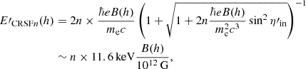 (7)
(7)
where n is the order of the Landau level, with n = 1 corresponding to the fundamental line, and η′in is the angle between the photon propagation direction and the B field (see, e.g., Mészáros 1992). As is seen from the exact part of Eq. (7) in question, the position of cyclotron resonances depends on the angle to the magnetic field and shows a slight anharmonicity due to relativistic effects (Harding & Daugherty 1991; Araya & Harding 1999). In reality, the centroid energy and shape of the resulting scattering features are determined by a complex resonant redistribution and affected by higher-order processes. The model of Schwarm et al. (2017a,b) considers these effects, demonstrating that redistribution and photon spawning can lead to stronger emission wings of the fundamental line and a reduction of its depths (see Schwarm et al. 2017a, for more details).
2.3. Neutron star rest frame
The specific intensity obtained from Eq. (5) is given in the local rest frame of the emitting plasma. In order to obtain the emission profile of the entire accretion column, we have to take into account the height dependence of the relativistic bulk motion. This means that we have to transform the local specific intensity emitted from different parts of the accretion column into a common frame of reference. An obvious choice for such a reference frame is the rest frame of the neutron star.
Transformation of the specific intensity from the local rest frame of the plasma (Eq. (5)) to the rest frame of the neutron star,
 (8)
(8)
is obtained through a Lorentz transformation,
 (9)
(9)
where the bulk velocity  . Note that the velocity vector is antiparallel to the B field. Starred quantities refer to the rest frame of the neutron star. We assume that the CRSF forming layer is coupled to the continuum emitting volume such that both have the same velocity and temperature distribution (Eq. (2)).
2.4. Geometry and ray tracing
In order to predict what the column would look like to an observer at infinity, we have to take into account general relativistic effects; specifically light bending, which also causes a lensing effect (solid angle amplification), and the gravitational redshift. Since our work focuses on accreting X-ray pulsars in high-mass X-ray binaries, we assumed that the neutron star is a slow rotator with a rotation period P ≲ 1 Hz, such that we could neglect time delays of observed photons, as well as the oblateness of the neutron star (the effects important for modeling fast rotators such as accreting millisecond pulsars Morsink et al. 2007; Bogdanov et al. 2019).
We used the developed ray-tracing code (see Sect. 1), which computes photon trajectories in the Schwarzschild metric and determines the observed energy- and phase-dependent flux, FE(ϕ), for arbitrary geometries (i.e., the location of the poles and the inclination of the rotation axis to the observer’s line of sight) and emission characteristics of the emission regions. We adopted a general approach based on the Schwarzschild metric, similar to Beloborodov (2002), Poutanen & Beloborodov (2006), and De Falco et al. (2016), who derived the observed flux for infinitesimal spots on a sphere. We extended this framework to include extended emission regions, including radial structure, as in the conical accretion column model Ferrigno et al. (2011). In this case, photon trajectories with a periastron cannot be ignored. The method, which is described in more detail in Appendix A, allows one to model arbitrary geometrical emission regions, without any required symmetry or other restrictions to the geometrical shape.
The ray-tracing code introduces additional parameters into the emission model. The most important one is the compactness of the neutron star, Rs/RNS, determined by the ratio of its Schwarzschild radius (Eq. (A.5)) and its radius. The compactness mainly influences the strength of the light bending – how much the photon trajectories differ from those in absence of any mass – and the gravitational redshift (Eq. (A.24)).
In addition to the compactness, the shape and location of the emission region have to be defined. In our case the shape of the cylindrical column is specified by the radius, rAC, and its height, hAC. As is discussed in Sect. 2.1, these parameters mainly depend on the initial free-fall velocity and Ṁ. The position of the column on the neutron star’s surface is given by its co-latitude ΘAC, that is, the inclination of the magnetic field, and its azimuthal angle ΦAC (Fig. 4) with respect to an arbitrary zero meridian on the neutron star’s surface. The azimuthal angle is only important when multiple columns are considered. In this case, it defines the angular offset between the columns. Here we assume that the B field axes pass through the center of mass; that is, that the accretion columns are perpendicular to the neutron star surface. An asymmetric B field would be accounted for by deviating from the antipodal case while still assuming the B field axis to be centered. Columns are antipodal if
 (10)
(10)
 |
Fig. 4. Geometry of a neutron star with two antipodal accretion columns sampled using triangular surface elements. The size of the surface elements is enhanced for visualization purposes. The inclination, i, of the observer is defined to lie on the x,z plane and measured with respect to the rotational axis z, as are the individual colatitudes of the accretion columns, ΘAC1 and ΘAC2. The azimuthal angles of both columns are designated ΦAC1 and ΦAC2. |
Finally, the inclination, i, of the observer’s line of sight relative to the neutron star’s rotational axis must be taken into account.
3. Results
The framework described above allows us to obtain the height-dependent radiation field from the column walls in the neutron star rest frame (Sect. 3.1) and the observed phase- and energy-dependent emission (Sect. 3.2).
3.1. Emission in the neutron star rest frame
Integrating the specific intensity over the whole height of the column and over all emission angles gives the total luminosity of the column in the energy band, E★min and E★max,
 (11)
(11)
In most cases considered here, the X-ray band from 1 keV to 100 keV approximately contains the total luminosity of the accretion column.
Figure 5 shows the height-dependent emission profile and other properties of the accretion column for the parameters listed in Table 1. The energy-integrated emission profiles are plotted as a function of height for several emission angles. All bin exhibit similar behavior, with peak emissivity occurring at the base of the column. Due to relativistic boosting, the relative contribution is clearly dominated by large angles (Fig. 5, left). The bulk velocity at the boundary layer is almost equal to the initial free-fall velocity for most parts of the column and only starts to decrease drastically h ∼ 100 m above the neutron star surface (Fig. 5, right). The electron temperature has a similar but smoother evolution as it is directly derived from the bulk velocity (Eq. (2)).
 |
Fig. 5. Height-dependent emission profile and properties of the (single) example accretion column of Fig. 3 in the rest frame of the neutron star. Left: Emission profile of the accretion column (Eq. (8)) integrated over the energy range from 1 to 100 keV in different μ★ bins, shown on a logarithmic scale. The inset shows the height- and energy-integrated beam pattern with respect to the angle η★. The colors correspond to the angle bins in the main figure (the yellow region is located at the very top of the beam pattern and is not visible at the chosen scale). The drop in flux to zero at the very base of the column follows from the adopted functional dependence on ∂Q/∂r (see Eq. (3)) and does not affect any of the presented results. Right: Velocity (solid black), temperature (dashed green), and magnetic field strength distribution (dash-dotted orange) at the boundary layer of the accretion column, i.e., r = r(τ⊥ = 1). |
Input parameters for the accretion column model.
For our (single) example column, the total intrinsic luminosity is L★ = 2.2 × 1037 erg s−1, of which 100% is emitted below a height of 5 km, 67% below 1 km, and 20% below 0.1 km (see Fig. 5, left). Therefore we can consider the column to have a height of hAC = 5 km. In the frame of the moving plasma, the emission is concentrated in the direction normal to the cylindrical column wall (Fig. 2). However, due to the boosting (relativistic aberration) caused by the bulk velocity, the emission in the frame of the star is predominantly directed downward; that is, toward the neutron star. In particular, 76% of the emission has an emission angle of η★ > 90° (or μ★ < 0).
Figure 6 shows the height-integrated spectra for emission from the column, using bins of the same angle as in Fig. 5. The spectra strongly depend on the emission angle. The shape of the CRSFs is largely determined by the behavior of the scattering cross section at a given emission angle, with the deepest and broadest profile occurring at smaller angles to the magnetic field (Fig. 6, yellow line). In the rest frame of the plasma, these correspond to directions close to the magnetic field, where the line shape experiences the strongest Doppler broadening due to electrons, moving freely along this axis. At larger angles to the magnetic field, line formation is accompanied by emergence of emission wings around the core (the effect is described in detail in, e.g., Isenberg et al. 1998; Schönherr et al. 2007; Schwarm et al. 2017a). Notably, the centroid energies of CRSFs also strongly depend on the emission angle. However, the visible increase in centroid energies at larger angles to the magnetic field cannot be explained by the angular dependence of the resonances in the cross sections, which predicts no significant variation for the fundamental and the opposite trend for higher harmonics (see, e.g., Eq. (7) and Schwarm et al. 2017b,a). This correlation results from the energy- and angle-dependent Lorentz boosting, which accounts for the CRSF formation in the moving medium of the column walls (Eq. (9)). The boosting also contributes to a mild hardening of the continuum at higher emission angles.
 |
Fig. 6. Angle-dependent spectra (Eq. (8)) of the example accretion column in the rest frame of the neutron star. Top: Height-integrated emerging spectra for the different emission angle ranges indicated in the inset (same as in Fig. 5). Bottom: Relative difference of the spectra to their pure continuum contribution. |
3.2. Observed emission
As was mentioned in Sect. 2.4, initiating a discussion on the observable properties of emission from accretion columns requires one to consider the geometrical properties of the emission regions, their locations, and the viewing angle of a remote observer relative to the neutron star’s rotation axis. This consideration significantly expands the parameter space. Our preliminary investigation indicates that this necessitates a systematic study, which will be the focus of Paper II. Here, we show a few immediate results for the directly observed column emission, which are readily accessible based on the discussion above.
As an example, Fig. 7 shows the observer’s view of a neutron star with two antipodal identical accretion columns, as well as their specific intensity in the observer’s frame, IE (Eq. (8) and Eq. (A.24)). Light bending enlarges the visible fraction of the neutron star, making it unlikely to observe only one pole (Ftaclas et al. 1986). In Fig. 7, the second column, partially hidden in flat space, becomes significantly more visible, contributing to phase- and energy-dependent emission.
 |
Fig. 7. Sky projection of a neutron star with two accretion columns observed at an inclination i = 80°. The two columns are located at (ΦAC1 = 37°, ΘAC1 = 50°) and (ΦAC2 = 143°, ΘAC2 = 130°). See Fig. 4 for an explanation of these angles. The colors encode the specific intensity, IE. We consider only the column wall emission. The top surface of the column is shown in white but does not emit. |
A given observer views various parts of the columns’ surfaces under different angles at a specific rotation phase. Together with the significant angle variability of the spectra (see Fig. 6), this leads to a complex energy-dependent behavior of the observed flux, FE(ϕ) (Eq. (A.32)). Figure 8 shows an example of the resulting pulse profiles at different energies for a chosen geometry, using the specific intensity, IE, determined from each emitting surface element. The normalization chosen for the profiles emphasizes their shape, rather than their absolute flux and their relative pulsed fraction. The shape strongly depends on the energy. In the soft X-ray band around ∼5 keV, below the fundamental CRSF, the pulse profile is double-peaked, without special features. At higher energies, however, the main peak is split by a dip, which becomes the global minimum at ∼90 keV. Changes in angular dependency between different continuum energies result mainly from the energy-dependent Lorentz transformations applied to the initially assumed fan-beam emission profile, as shown in Fig. 6 for the neutron star rest frame. However, the behavior of the flux in the observer’s frame additionally includes mixed contributions from different heights of the column and visibility effects. The pronounced dips at higher energies are caused by the occultation by the neutron star of the hot bottom part of the column, emitting harder radiation. This and other visibility effects are geometry-dependent and are addressed in detail in Paper II.
 |
Fig. 8. Energy-dependent pulse profiles normalized by their standard deviation, σFE, using the specific intensity, IE, calculated with parameters given in Table 1. The B field of the two antipodal columns is inclined by ΘAC1 = 46° and ΘAC2 = 134°, respectively, while i = 78°. |
Figure 9 shows energy-integrated pulse profiles for the same observer’s viewing angle but different locations of the two antipodal columns. Even in this case, the geometry produces a variety of pulse shapes. At small ΘAC1, the pulse profiles show a single broad peak at ϕ = 0, while for larger ΘAC1 a second peak develops at ϕ = 0.5. Increasing ΘAC1, bringing it closer to i, also leads to the formation of shoulders on the main or secondary peaks. The contribution of the main peak (ϕ = 0) increases significantly at ΘAC1 ∼ i (the effect was discussed previously for physical and phenomenological column emission models; see, e.g., Meszaros & Riffert 1988; Nollert et al. 1989; Markozov & Mushtukov 2024). These basic examples demonstrate that the observed flux is strongly dependent on energy and the underlying geometry, which can be used to constrain the pole location and the observer’s viewing angle. This problem is further explored in Paper II.
 |
Fig. 9. Energy-integrated pulse profiles normalized by their standard deviation, σFE, for different antipodal two-column geometries with varying B field inclinations ΘAC1, 2 for the model column with parameters given in Table 1. |
4. Summary and outlook
In this paper, we present a framework for computing the energy- and phase-dependent X-ray flux from accreting neutron stars. The model consists of three key components, each capturing distinct physical aspects within and around the accretion column. We illustrate this approach by obtaining the conditions within the accretion column, its dimensions, and its continuum emission using the model of Postnov et al. (2015) with CRSFs imprinted based on Schwarm et al. (2017a,b) and take into account the bulk motion in the column’s outer layer. The resulting radiation field is then transformed into the observer frame using general relativistic ray tracing. The developed methodology integrates components, which are crucial to narrowing the gap between emission models and the accumulated multidimensional observational data.
This model allows us to investigate the scenario, when CRSFs originate in the side-wall emission. Some modification of the spectra by imprinted CRSFs are visible at all emission angles. The position of the lines and their shape depends dramatically on the angle, owing to the combination of Doppler broadening in the rest frame of the plasma and Lorenz boosting due to the formation in a fast-moving outer layer of the column. A very pronounced absorption feature appears only in the directions closer to the magnetic field, where the overall flux is significantly reduced. We would like to note that the second harmonic is very weak in this case and most likely would not be visible after taking into account a detection process. The contribution of various angular beams to the total flux, and thus the observability of the features, depends further on the geometry and is addressed in Paper II.
As was mentioned earlier, the fast-moving outer layer in an accretion column is a common result of two-dimensional hydrodynamic and magneto-hydrodynamic simulations (see, e.g., Gornostaev 2021; Zhang et al. 2022; Sheng et al. 2023). However, resonant processes are generally not included in detail in such simulations, as they dramatically increase computational costs. Sheng et al. (2023) accounted for angle- and energy-averaged magnetic opacities in the accretion column, which results in a significant difference in column structure and dynamics compared to earlier work (Zhang et al. 2022). The general behavior of the horizontal velocity profile, with the fast-moving outer layer, is typically preserved. It remains unclear, however, whether proper inclusion of intense resonant scattering in this layer would affect this general picture. In this way, the combined model used in this work provides a physical description of the accretion column’s emission that is consistent with the state of the art in the field and is compatible with the requirements of the ray-tracing code presented here. However, we note that such dynamical effects as photon bubbles described for nonstationary calculations can modify the structure of the accretion mound and also allow radiation to escape without reprocessing in the free-falling region (Klein et al. 1996; Klein 1997; Zhang et al. 2022, 2023).
The modularity of our approach also has some limitations, especially at the interfaces of the continuum and the CRSF model, where an abrupt transition is implied between the two regions. As discussed in Sect. 2.1, the continuum is formed at the surface of constant optical depth, τ⊥ = 1 (Postnov et al. 2015). The CRSF model of Schwarm et al. (2017a,b), however, assumes a very thin outermost layer that has an optical depth of ∼10−4. Nevertheless, we assume the electron temperature and the bulk velocity to be the same in both layers as the spatial separation is negligible. We also neglect the vertical redistribution of photons due to the vertical discretization of the column. Furthermore, the model by Postnov et al. (2015) used for the continuum emission is based on Lyubarskii (1986), who considered the photon energy to be smaller than the fundamental CRSF energy, which itself is assumed to exceed the electron temperature, i.e., E′ ≪ E′CRSF1 and E′CRSF1 ≫ kT. While the second condition is met, the first one is only partially fulfilled. As a consequence, the contribution of ordinary photons to the continuum especially at higher energies is underestimated. An estimate of this deviation would only be possible using a more sophisticated description of the accretion column emission.
In our model, a significant amount of radiation emitted by the accretion column (∼58%) is intercepted by the neutron star surface. This irradiation of a neutron star due to a bulk motion in the accretion channel was first described by Kaminker et al. (1976) and was later proposed by Poutanen et al. (2013) as a key factor in explaining the correlation of CRSF energy and X-ray luminosity. While the re-emission (“reflection”) component can be straightforwardly incorporated in our setup, calculating a physically motivated spectral and angular distribution for this component is a complex task. This will be addressed in future work, while the discussion here and in Paper II is limited to directly observable emission from the accretion column as a foundation for further development. It is also important to note that the approach used here to account for the presence of the bulk flow is oversimplified. In reality, even when the emission predominantly escapes from the column wall, not all photons emitted and up-scattered by thermal electrons in the settling interior of the column interact with the fast-moving flow at the boundary. In this way, the effect of the downward boosting of the continuum in our model is likely overestimated (see, also, Kylafis et al. 2021, for the related discussion).
Currently, we do not include the treatment of polarization in our setup. Polarization is an important dimension of the problem, and polarization effects in a strong magnetic field are crucial for understanding emission formation (Mészáros 1992). Properly accounting for photon polarization modes in the observed emission requires one to consider photon propagation effects in the neutron star magnetosphere, which can modify the polarization signal (see, e.g., Wang & Lai 2009 and, for ultra-strong fields, Shaviv et al. 1999). This requires a different treatment of ray tracing and will be addressed in future studies.
A detailed discussion of the directly observable emission from an accretion column, as predicted by the model described here, is given in Paper II. There we present a set of energy- and phase-dependent implications and predictions relevant for interpreting observational data. The primary focus is the dependence of these observables on the geometry – the inclination of the observer’s line of sight and the location of the accretion columns. The resulting angle- and energy-dependent flux has to be investigated in the systematic manner due to a complex parameter space and warrants a separate discussion.
Data availability
The ray-tracing code is written in ISIS and is available at https://www.sternwarte.uni-erlangen.de/research/lbscripts. The current setup is complex, as required by the broad ranges of the code applicability, and is not efficient enough to be used directly for pulse profile or spectral fits (all related examples mentioned in Sect. 1 relied on a set of model-specific interpolation tables). Nevertheless, it serves as a robust foundation for exploring the interplay between emission characteristics and geometry, as well as a prototype for simpler models with stricter assumptions and higher computational performance (e.g., Thalhammer et al. 2024).
Acknowledgments
We dedicate this work to the memory of our beloved colleagues, Dr. Katja Pottschmidt and Dr. Maurizio Falanga, who unexpectedly passed away last year. They provided invaluable contributions to this study, and their work continues to be an integral part of this paper. We thank the anonymous referee for their constructive comments, which helped to improve the clarity and quality of this manuscript. This work has been funded by the Deutsche Forschungsgemeinschaft under the DFG grant number WI 1820-10/1. The work of KP is supported by RFBR grant 18-502-12025. The work of ESL is also supported by the FAU Emerging Talents Initiative. The material is based upon work supported by NASA under award number 80GSFC21M0002. Astrophysics research at the Naval Research Laboratory is supported by the NASA Astrophysics Explorer Program. The authors are grateful to M. Gornostaev, M. Sasaki, and J. J. R. Stierhof for valuable comments and discussions. The fruitful discussions within the XMAG (former MAGNET) collaboration also had a very positive impact on this work. We acknowledge the support from the Faculty of the European Space Astronomy Centre (ESAC). This research has made use of ISIS functions (ISISscripts) provided by ECAP/Remeis observatory and MIT (http://www.sternwarte.uni-erlangen.de/isis/). The figures in this work have been produced with the S-Lang module slxfig developed by J. Davis.
References
- Araya, R. A., & Harding, A. K. 1999, ApJ, 517, 334 [NASA ADS] [CrossRef] [Google Scholar]
- Arons, J., Klein, R. I., & Lea, S. M. 1987, ApJ, 312, 666 [Google Scholar]
- Bakala, P., Bakalová, A., La Placa, R., Falanga, M., & Stella, L. 2023, A&A, 673, A164 [NASA ADS] [CrossRef] [EDP Sciences] [Google Scholar]
- Basko, M. M., & Sunyaev, R. A. 1976, MNRAS, 175, 395 [Google Scholar]
- Becker, P. A., & Wolff, M. T. 2007, ApJ, 654, 435 [NASA ADS] [CrossRef] [Google Scholar]
- Becker, P. A., Klochkov, D., Schönherr, G., et al. 2012, A&A, 544, A123 [NASA ADS] [CrossRef] [EDP Sciences] [Google Scholar]
- Beloborodov, A. M. 2002, ApJ, 566, L85 [Google Scholar]
- Bogdanov, S., Lamb, F. K., Mahmoodifar, S., et al. 2019, ApJ, 887, L26 [NASA ADS] [CrossRef] [Google Scholar]
- Burnard, D. J., Arons, J., & Klein, R. I. 1991, ApJ, 367, 575 [CrossRef] [Google Scholar]
- Caballero, I., & Wilms, J. 2012, Mem. Soc. Astron. It., 83, 230 [NASA ADS] [Google Scholar]
- Canuto, V., Lodenquai, J., & Ruderman, M. 1971, Phys. Rev. D, 3, 2303 [NASA ADS] [CrossRef] [Google Scholar]
- Cappallo, R., Laycock, S. G. T., & Christodoulou, D. M. 2017, Publ. Astron. Soc. Pac., 129, 124201 [Google Scholar]
- Davidson, K. 1973, Nat. Phys. Sci., 246, 1 [NASA ADS] [CrossRef] [Google Scholar]
- De Falco, V., Falanga, M., & Stella, L. 2016, A&A, 595, A38 [NASA ADS] [CrossRef] [EDP Sciences] [Google Scholar]
- Falkner, S. 2013, Master’s Thesis, Friedrich-Alexander-Universität Erlangen-Nürnberg, Germany [Google Scholar]
- Falkner, S. 2018, dissertation, Friedrich-Alexander-Universität Erlangen-Nürnberg, Germany [Google Scholar]
- Falkner, S., Sokolova-Lapa, E., Schwarm, F.-W., et al. 2026, A&A, 711, A225 (Paper II) [NASA ADS] [CrossRef] [EDP Sciences] [Google Scholar]
- Ferrigno, C., Falanga, M., Bozzo, E., et al. 2011, A&A, 532, A76 [CrossRef] [EDP Sciences] [Google Scholar]
- Ferrigno, C., D’Aì, A., & Ambrosi, E. 2023, A&A, 677, A103 [NASA ADS] [CrossRef] [EDP Sciences] [Google Scholar]
- Fotiadis, P., Loudas, N., Kylafis, N. D., & Trümper, J. 2026, A&A, 709, A247 [NASA ADS] [CrossRef] [EDP Sciences] [Google Scholar]
- Ftaclas, C., Kearney, M. W., & Pechenick, K. 1986, ApJ, 300, 203 [Google Scholar]
- Gornostaev, M. I. 2021, MNRAS, 501, 564 [Google Scholar]
- Gornostaev, M. I. 2025, MNRAS, 544, 3229 [Google Scholar]
- Harding, A. K., & Daugherty, J. K. 1991, ApJ, 374, 687 [NASA ADS] [CrossRef] [Google Scholar]
- Isenberg, M., Lamb, D. Q., & Wang, J. C. L. 1998, ApJ, 505, 688 [NASA ADS] [CrossRef] [Google Scholar]
- Iwakiri, W. B., Pottschmidt, K., Falkner, S., et al. 2019, ApJ, 878, 121 [NASA ADS] [CrossRef] [Google Scholar]
- Kaminker, A. D., Fedorenko, V. N., & Tsygan, A. I. 1976, Sov. Astron., 20, 436 [NASA ADS] [Google Scholar]
- Klein, R. I. 1997, in Computational Astrophysics; 12th Kingston Meeting on Theoretical Astrophysics, eds. D. Clarke, & M. West, 12, 55 [Google Scholar]
- Klein, R. I., & Arons, J. 1989, in Two Topics in X-Ray Astronomy, Volume 1: X Ray Binaries. Volume 2: AGN and the X Ray Background, eds. J. Hunt, & B. Battrick, 1, 89 [Google Scholar]
- Klein, R. I., Arons, J., Jernigan, G., & Hsu, J. J. L. 1996, ApJ, 457, L85 [Google Scholar]
- Kumar, S., Bala, S., & Bhattacharya, D. 2022, MNRAS, 515, 914 [CrossRef] [Google Scholar]
- Kylafis, N. D., Trümper, J. E., & Loudas, N. A. 2021, A&A, 655, A39 [NASA ADS] [CrossRef] [EDP Sciences] [Google Scholar]
- La Placa, R., Bakala, P., Stella, L., & Falanga, M. 2019, Res. Notes Am. Astron. Soc., 3, 99 [Google Scholar]
- Lamb, F. K., Pethick, C. J., & Pines, D. 1973, ApJ, 184, 271 [NASA ADS] [CrossRef] [Google Scholar]
- Loudas, N., Kylafis, N. D., & Trümper, J. 2024, A&A, 689, A75 [NASA ADS] [CrossRef] [EDP Sciences] [Google Scholar]
- Lutovinov, A. A., Tsygankov, S. S., Suleimanov, V. F., et al. 2015, MNRAS, 448, 2175 [NASA ADS] [CrossRef] [Google Scholar]
- Lyubarskii, Y. É. 1986, Astrophysics, 25, 577 [Google Scholar]
- Markozov, I. D., & Mushtukov, A. A. 2024, MNRAS, 527, 5374 [Google Scholar]
- Markozov, I. D., Kaminker, A. D., & Potekhin, A. Y. 2024, Astron. Lett., 49, 583 [Google Scholar]
- Mészáros, P. 1992, High-energy Radiation from Magnetized Neutron Stars (Chicago: University of Chicago Press) [Google Scholar]
- Meszaros, P., & Nagel, W. 1985a, ApJ, 298, 147 [NASA ADS] [CrossRef] [Google Scholar]
- Meszaros, P., & Nagel, W. 1985b, ApJ, 299, 138 [NASA ADS] [CrossRef] [Google Scholar]
- Meszaros, P., & Riffert, H. 1988, ApJ, 327, 712 [Google Scholar]
- Mészáros, P., & Ventura, J. 1978, Phys. Rev. Lett., 41, 1544 [CrossRef] [Google Scholar]
- Misner, C. W., Thorne, K. S., & Wheeler, J. A. 1973, Gravitation (San Francisco: W.H. Freeman and Co.) [Google Scholar]
- Morsink, S. M., Leahy, D. A., Cadeau, C., & Braga, J. 2007, ApJ, 663, 1244 [NASA ADS] [CrossRef] [Google Scholar]
- Mushtukov, A., & Tsygankov, S. 2023, in Handbook of X-ray and Gamma-ray Astrophysics, eds. C. Bambi, & A. Santangelo (Singapore: Springer Nature), 1 [Google Scholar]
- Mushtukov, A. A., Tsygankov, S. S., Serber, A. V., Suleimanov, V. F., & Poutanen, J. 2015, MNRAS, 454, 2714 [Google Scholar]
- Nishimura, O. 2014, ApJ, 781, 30 [NASA ADS] [CrossRef] [Google Scholar]
- Nollert, H. P., Ruder, H., Herold, H., & Kraus, U. 1989, A&A, 208, 153 [Google Scholar]
- Pavlov, G. G., Shibanov, I. A., & Iakovlev, D. G. 1980, Ap&SS, 73, 33 [Google Scholar]
- Pechenick, K. R., Ftaclas, C., & Cohen, J. M. 1983, ApJ, 274, 846 [Google Scholar]
- Postnov, K. A., Gornostaev, M. I., Klochkov, D., et al. 2015, MNRAS, 452, 1601 [Google Scholar]
- Poutanen, J. 2020, A&A, 640, A24 [NASA ADS] [CrossRef] [EDP Sciences] [Google Scholar]
- Poutanen, J., & Beloborodov, A. M. 2006, MNRAS, 373, 836 [NASA ADS] [CrossRef] [Google Scholar]
- Poutanen, J., Mushtukov, A. A., Suleimanov, V. F., et al. 2013, ApJ, 777, 115 [NASA ADS] [CrossRef] [Google Scholar]
- Rebetzky, A., Bock, U., Herold, H., Kraus, U., & Maile, T. 1989, A&A, 225, 137 [Google Scholar]
- Schönherr, G., Wilms, J., Kretschmar, P., et al. 2007, A&A, 472, 353 [NASA ADS] [CrossRef] [EDP Sciences] [Google Scholar]
- Schwarm, F.-W., Ballhausen, R., Falkner, S., et al. 2017a, A&A, 601, A99 [NASA ADS] [CrossRef] [EDP Sciences] [Google Scholar]
- Schwarm, F.-W., Schönherr, G., Falkner, S., et al. 2017b, A&A, 597, A3 [NASA ADS] [CrossRef] [EDP Sciences] [Google Scholar]
- Shaviv, N. J., Heyl, J. S., & Lithwick, Y. 1999, MNRAS, 306, 333 [Google Scholar]
- Sheng, X., Zhang, L., Blaes, O., & Jiang, Y.-F. 2023, MNRAS, 524, 2431 [NASA ADS] [CrossRef] [Google Scholar]
- Sokolova-Lapa, E. 2023, dissertation, Friedrich-Alexander-Universität Erlangen-Nürnberg, Germany [Google Scholar]
- Staubert, R., Shakura, N. I., Postnov, K., et al. 2007, A&A, 465, L25 [NASA ADS] [CrossRef] [EDP Sciences] [Google Scholar]
- Staubert, R., Trümper, J., Kendziorra, E., et al. 2019, A&A, 622, A61 [NASA ADS] [CrossRef] [EDP Sciences] [Google Scholar]
- Steiner, A. W., Lattimer, J. M., & Brown, E. F. 2013, ApJ, 765, L5 [Google Scholar]
- Thalhammer, P., Ballhausen, R., Sokolova-Lapa, E., et al. 2024, A&A, 688, A213 [NASA ADS] [CrossRef] [EDP Sciences] [Google Scholar]
- Tsygankov, S. S., Lutovinov, A. A., & Serber, A. V. 2010, MNRAS, 401, 1628 [NASA ADS] [CrossRef] [Google Scholar]
- Wang, Y.-M., & Frank, J. 1981, A&A, 93, 255 [NASA ADS] [Google Scholar]
- Wang, C., & Lai, D. 2009, MNRAS, 398, 515 [Google Scholar]
- Zhang, L., Blaes, O., & Jiang, Y.-F. 2022, MNRAS, 515, 4371 [NASA ADS] [CrossRef] [Google Scholar]
- Zhang, L., Blaes, O., & Jiang, Y.-F. 2023, MNRAS, 520, 1421 [CrossRef] [Google Scholar]
The constant factor of 3/7π in Eq. (1) is chosen such that  .
.
Ferrigno et al. (2011) stated that σ1 = σ2 = 45°, which, however, does not match the corresponding emission pattern in their Fig. 9 (C. Ferrigno, priv. comm.).
Appendix A: Ray tracing method
In this appendix we describe the ray tracing method used in this work. While much of the underlying calculations were already presented in the literature, the notations used in the relevant papers are inconsistent with each other. This makes implementations of these theories error prone. Here, we summarize the literature in a consistent way. We give the mathematical formulation in Sect. A.1 through A.4. In Sect. A.5 we then outline the numerical implementation. In Sect. A.6 we verify the validity of our ray tracing method by comparing our results to Ferrigno et al. (2011).
A.1. Equations of motion
Solving the geodesic equation based on the Schwarzschild metric in spherical coordinates (t, r, θ, ψ) yields the equations of motion for photons. In particular, exploiting spherical symmetry and the conservation of angular momentum (θ ≡ π/2), the components of the photon’s four-velocity can be written as (see, e.g., Misner et al. 1973)
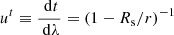 (A.1)
(A.1)
![Mathematical equation: $$ \begin{aligned} u^r \equiv \frac{\ \mathrm{d}{r}}{\ \mathrm{d}{\lambda }}&= \left[ 1-b^2\left(1-{R_\mathrm{s} }/r\right)/r^2 \right]^{1/2}\end{aligned} $$](/articles/aa/full_html/2026/07/aa53642-24/aa53642-24-eq15.gif) (A.2)
(A.2)
 (A.3)
(A.3)
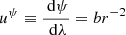 (A.4)
(A.4)
where
 (A.5)
(A.5)
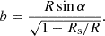
is the Schwarzschild radius for a neutron star of mass MNS, and where b the impact parameter, i.e., the distance between the trajectory and the line of sight, which connects the center of the neutron star and the observer (Fig. A.1). The impact parameter can be expressed in terms of the radial emission angle α, i.e., the angle between the radial position vector, n, and the initial emission direction of the photon, k★. With Eqs. (A.2–A.4),
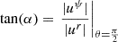 (A.6)
(A.6)
 |
Fig. A.1. Visualization of the ray tracing parametrization. The orange solid line represents the trajectory of photons emitted at (R, φ, ϑ) in the direction k★ with the emission angle α with respect to the radial vector n. R represents the radius of emission. The photon reaches the observer plane (at infinity) at the impact point (A = b cos ρ, B = b sin ρ) at a distance b. The direction k toward the observer is defined to lie in the x, z-plane, inclined by the inclination i with respect to the z-axis, which is also the axis of rotation. The angle between n and k is the apparent emission angle Ψ. The magenta dashed line represents the second possible trajectory, Ψ∗, to the observer of a photon emitted at (R, φ, ϑ). In this case the photon is emitted toward the neutron star, that is, α > 90° and exhibits a periastron at (Rp,Ψp). |
such that
 (A.7)
(A.7)
The trajectory of the photon can then be described by the elliptical integral
![Mathematical equation: $$ \begin{aligned} \begin{aligned} \psi _b(R)&= \int _R^\infty \frac{\ \mathrm{d}{\psi }}{\ \mathrm{d}{\lambda }}\frac{\ \mathrm{d}{\lambda }}{\ \mathrm{d}{r}}\ \mathrm{d}{r}\\&= \int _R^\infty \frac{\ \mathrm{d}r}{r^2} \left[ \frac{1}{b^2} - \frac{1}{r^2}\left(1-\frac{{R_\mathrm{s} }}{r}\right)\right]^{-1/2}, \end{aligned} \end{aligned} $$](/articles/aa/full_html/2026/07/aa53642-24/aa53642-24-eq21.gif) (A.8)
(A.8)
where ψ is the polar angle between the direction to the observer at infinity and the current location R of the photon (see Fig. A.1). Note that R is not necessarily equal to the radius of the neutron star, RNS, i.e., R ≥ RNS.
Those trajectories in Eq. (A.8) for which α ≥ 90°, i.e., photons emitted toward the neutron star, can exhibit a periastron at
![Mathematical equation: $$ \begin{aligned} R_\mathrm{p} (b) = -2\sqrt{\frac{b^2}{3}}\cos \left[\frac{1}{3}\arccos \left(\frac{3\sqrt{3}}{2}\frac{{R_\mathrm{s} }}{b}\right) +\frac{2\pi }{3} \right], \end{aligned} $$](/articles/aa/full_html/2026/07/aa53642-24/aa53642-24-eq22.gif) (A.9)
(A.9)
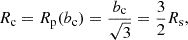
where α = 90° corresponds to the periastron itself. Equation (A.9) is only valid for b > bc, with the critical impact parameter
 (A.10)
and the critical radius
 (A.11)
below which photon trajectories do not exhibit a periastron and spiral inward to the center of mass. From Eq. (A.7) we derive the maximum radial emission angle,
 (A.12)
To account for periastra, the photon trajectory in Eq. (A.8) has to be considered, such that
 (A.13)
A.2. Analytic approximations
Beloborodov (2002) presents an accurate analytical approximation for the photon trajectory defined by Eq. (A.8) given by
 (A.14)
which De Falco et al. (2016) derive in a more general approach. This approximation requires that R > 2Rs = Rcapprox. Note that the critical radius in this approximation is larger than that in the exact solution (Eq. A.11). In other words, in the approximation of Beloborodov (2002) a neutron star with a radius of 2Rs would look like a neutron star of radius  based on the exact calculation. Objects therefore appear to be more compact when using the approximate solution rather than the exact calculation. In contrast, the relative deviation of the bending angle, ξ = Ψ − α, which is the most crucial parameter for ray tracing, deviates only by at most 10% from the exact solution (Fig. A.2). This maximum relative deviation is reached only for the extreme case of α → αmax (Eq. A.12).
 |
Fig. A.2. Accuracy of the analytical photon trajectory approximation (Eq. A.14). This figure is similar to Beloborodov (2002, Fig. 2) and shows contour lines (solid, dotted) of constant deviation δξ/ξ of the bending angle ξ = Ψ − α of the analytical approximation (Eq. A.14) to the exact solution (Eq. A.13). The black and purple shaded regions relate to the maximum radial emission angles, αmax and αmaxapprox, for the exact and approximated case, respectively. The orange shaded area confines the region that can be occupied by a neutron star with MNS = 1.4 M⊙ (see, e.g., Steiner et al. 2013). Note that the y-axis of Beloborodov (2002, Fig. 2) actually begins at Rs/R = 0.01 and not at 0 as implied in their figure. |
For α ≤ 90° the accuracy map in Fig. A.2 matches that of Beloborodov (2002, their Fig. 2), which shows the correctness of our numerical calculation of the photon trajectory given by Eq. (A.13). Note that as expected we obtain δξ = 0 for Rs/R → 0 and arbitrary α, as the apparent and radial emission angle are equal, i.e., α = Ψ.
Several more accurate approximations for the bending angle and amplification factor in the Schwarzschild field have been proposed in recent years, many of which improve the treatment of trajectories with a periastron (see, e.g., La Placa et al. 2019; Poutanen 2020; Bakala et al. 2023). We expect that integrating some of these approximations into the ray-tracing code will improve computational performance without a significant loss of accuracy.
A.3. Sky projection
By setting θ ≡ π/2 in the geodesic equations in Eqs. (A.1–A.4) we can reduce the three dimensional problem into a plane, where a trajectory can be identified only by its impact parameter b. To obtain the projected image in the observer plane we need to introduce another variable. The azimuthal angle ρ in the observer plane allows us to define the impact point (X, Y) of a photon trajectory in the observer plane (see Fig. A.1) as
 (A.15)
where ρ is defined by
![Mathematical equation: $$ \begin{aligned} \begin{aligned} \cos \rho&= \frac{\left[\boldsymbol{k}\times \left(\boldsymbol{n}\times \boldsymbol{k}\right)\right]\cdot \boldsymbol{e}_y}{ \left|\boldsymbol{k}\times \left(\boldsymbol{n}\times \boldsymbol{k}\right)\right|}\\&= \frac{\sin \vartheta \sin \varphi }{\sqrt{\sin ^2\vartheta \sin ^2\varphi + (\sin i\cos \vartheta -\cos i\sin \vartheta \cos \varphi )^2}} \end{aligned} \end{aligned} $$](/articles/aa/full_html/2026/07/aa53642-24/aa53642-24-eq30.gif) (A.16)
(A.16)
and
![Mathematical equation: $$ \begin{aligned} \begin{aligned} \sin \rho&= \frac{\left|\left[\boldsymbol{k}\times \left(\boldsymbol{n}\times \boldsymbol{k}\right)\right] \times \boldsymbol{e}_y\right|}{ \left|\boldsymbol{k}\times \left(\boldsymbol{n}\times \boldsymbol{k}\right)\right|}\\&= \frac{\sin i\cos \vartheta - \cos i\sin \vartheta \cos \varphi }{ \sqrt{\sin ^2\vartheta \sin ^2\varphi +(\sin i\cos \vartheta -\cos i\sin \vartheta \cos \varphi )^2}}\ , \end{aligned} \end{aligned} $$](/articles/aa/full_html/2026/07/aa53642-24/aa53642-24-eq31.gif) (A.17)
(A.17)
where
 (A.18)
is the direction vector to the observer, which is inclined to the z-axis by the inclination angle i. The angle ψ is geometrically described by
 (A.19)
The initial emission direction k★ can be expressed as
 (A.20)
Note that in case of geometrical projection in flat spacetime. k★ = k as Ψ = α. Finally, we can express the solid angle occupied by an infinitesimal spot dS for an observer at distance D in terms of the impact parameters,
 (A.21)
A.4. Flux determination
Using the above definitions we can determine the energy- and phase-resolved flux observed from the neutron star. In order to do so, we need to integrate the specific intensity, IE, as measured in the observer’s rest frame over the solid angle in the observer’s sky, Ω, that is occupied by the surface of the emitting area, S, at rotational phase ϕ,
 (A.22)
While the geometry of the emitting surface, S, may be static, the corresponding solid angle, which represents the projection of the surface element on the observer’s sky, depends on the rotational phase and the line of sight, i.e., Ω = Ω(S, ϕ, k) (Eq. A.21).
The transformation between the specific intensity in the rest frame of the accretion column and that in the observer rest frame is analog to Eq. (8), i.e.,
 (A.23)
where
 (A.24)
refers to the gravitational redshift z of a photon that is emitted at the radius R away from the center of mass. Equation (A.20) transforms between the observed, k, and the intrinsic emission direction, k★, of the photon.
A.5. Numerical procedure
Figure A.3 gives an overview of the numerical procedure that implements the steps outlined in the previous sections. We first define the geometrical setup, i.e., mass, MNS, and radius, RNS, of the neutron star, and the spatial extent of the emission region and its location. As indicated in Fig. 4, using an approach common in computer graphics, we achieve the independence of symmetry requirements by sampling the emitting region with a mesh of small triangular surface elements. In particular, we sample the surface S of the emitting region with a set of vertices Rl(R, φ(ϕ),ϑ), where l ∈ L ⊂ ℕ and |L| depends on the chosen resolution. These vertices are forming a mesh of triangular surface elements
 (A.25)
 |
Fig. A.3. Flow chart sketching the steps of the numerical procedure of the relativistic ray tracing method (see Sect. A.5). As a first step the geometrical setup, the emitting surface, is defined by a mesh of triangular surface elements. Additionally an interpolation table has to be provided, which contains information of possible photon trajectories. Based on these inputs the main step, the projection onto the observer sky, can be performed. In this step the two solutions for trajectories are determined and saved if valid for each phase ϕ and for each surface element n. In an optional step (dashed arrows) overlapping projections are filtered. In the end the given specific intensity is applied to the valid projections of each individual surface element and the resulting overall observed flux is determined. |
such that each normal vector points outward and their sum adds up to the area of the emission region, i.e, ∑n|ΔSn|=S, where n numbers the surface elements and nm ∈ L with m ∈ {0, 1, 2} indicates the corresponding vertices. Note that each vector Rl can be a vertex in several (up to six) surface elements. The vertex coordinate
 (A.26)
depends on the initial azimuthal position φ0 = φ(0) and on the rotational phase ϕ (see Fig. A.1). There are no restrictions or requirements to the shape of the emitting surface, except for R > Rc.
A pre-calculated interpolation table (Fig. A.3) is used to perform the relativistic projection. This projection is represented by the solid angle Ω corresponding to the emitting surface S. Based on the position of the neutron star with respect to the observer, which is determined by the radius R and the angle Ψ, we calculate the light bending parameters (b, α) required for the projection. The tabulation step is necessary as the calculation of photon trajectories exhibiting a periastron requires the periastron to be known beforehand (see Eq. A.13). The periastron, however, is determined by the impact parameter, b, of the trajectory (see Eq. A.9), while the calculation of b requires the emission angle α and the emission radius R (Eq. A.7). Using Eq. (A.7) and Eq. (A.13) we therefore calculate b and Ψ for given sets of R and α, which together provide the interpolation table. To improve the efficiency the radial range of the table can be limited to the geometric extent of the given setup.
The main step of the numerical procedure is the projection of the 3-dimensional geometrical structure onto the observer sky as a function of the rotational phase (Fig. A.3). This projection is given by the solid angles, ΔΩn, occupied by the corresponding surface elements, ΔSn. The numerical approximation of the solid angle in Eq. (A.21) is
![Mathematical equation: $$ \begin{aligned} \Delta \Omega _n&= \frac{1}{2D^2}\left[(X_{n_2}-X_{n_0})(Y_{n_1}-Y_{n_0})\right. - \nonumber \\&\,\quad \qquad \qquad \qquad \quad \qquad \left.(X_{n_1}-X_{n_0})(Y_{n_2}-Y_{n_0})\right]. \end{aligned} $$](/articles/aa/full_html/2026/07/aa53642-24/aa53642-24-eq41.gif) (A.27)
(A.27)
that is, the triangular area enclosed by the impact points (Xnm, Ynm) in the observer plane corresponding to the vertex set Rnm forming the surface element ΔSn.
The calculation of the solid angles for the determination of the pulse profiles is performed in a series of steps defined by a grid of rotational phases, ϕj. At each phase only a subset of the surface elements has a valid projection. The individual steps and different criteria for a valid projection at a given phase are described in the following.
First, using Eq. (A.19) we determine Ψnm for all according vertex sets nm based on the line of sight, k, and the current location, Rnm. for the two possible trajectory sets, Ψnm and 2π − Ψnm (see Fig. A.1) we can then look up the corresponding ray tracing parameters, bnm and αnm in the interpolation table. Both solutions are checked for validity. A trajectory set is dismissed if it intersects with the neutron star surface, that is, if for any nm
 (A.28)
or equivalently
 (A.29)
In this case, the corresponding surface element, ΔSn, would be at least partially invisible. To obtain the initial photon emission direction k★n for each valid solution, single ray tracing parameters are determined by averaging according to
 (A.30)
From Eq. (A.20) we then obtain the corresponding initial emission direction, k★n, and the emission angle, ηn, relative to the surface normal vector, where
 (A.31)
Surface elements with relative emission angles ηn > 90°, i.e., trajectories pointing inward into the emitting surface, are again dismissed. As a result, at a given phase, for each surface element, ΔSn, there are either no, one, or two projections, ΔΩn. The latter case is very unlikely and requires a special kind of geometry with surface elements with normal vectors pointing toward the neutron star surface, for example an emission region detached from the neutron star surface.
An optional step is to check for overlapping projections (Fig. A.3), i.e., solid angles ΔΩn that (partially) occupy the same area in the observer sky. This check is very time consuming and unnecessary in most cases. An example are solid columns, which are located roughly on opposite sides of the neutron star. Their projections do not occupy the same area at any phase (see, e.g., Fig. 7). For hollow columns or columns located very close to each other, however, it is likely that there are photon trajectories, which are intercepted by another part of the emission region. In such cases, adjacent solid angles in the observer’s sky have to be checked for overlaps and those shadowed by another are tagged as invalid.
Finally, at each phase and for each surface element with at least one valid solution we determine the observed flux from a simple numerical approximation of Eq. (A.22),
 (A.32)
A.6. Code verification
In order to verify our approach we compare our results with those of Ferrigno et al. (2011), who presented semi-analytical pulse profiles for conical accretion columns, accounting for light bending. These authors use a mixture of two Gaussians as the emission pattern
![Mathematical equation: $$ \begin{aligned} I_\mathrm{Ferringo} ^{\star }(\alpha ) = \sum _{j=1}^2 N_j \exp \left[-\frac{1}{2}\left(\frac{\alpha -\alpha _j}{\sigma _j}\right)^2\right], \end{aligned} $$](/articles/aa/full_html/2026/07/aa53642-24/aa53642-24-eq47.gif) (A.33)
(A.33)
with α1 = 150°, α2 = 0° and σ1 = σ2 = 28°.2 To test our ray tracing method we used the same setup of two conical accretion columns of the same height and opening angle asymmetrically placed on the canonical neutron star. The comparison of the resulting pulse profiles is shown in Fig. A.4. With deviations less than 2% the results agree very well.
 |
Fig. A.4. Normalized pulse profiles in comparison. Dashed gray lines relate to calculations by Ferrigno et al. (2011, bottom right panel in their Fig. 9) and solid lines to the numerical ray tracing method presented here. Red and blue corresponds to the contribution of the two conical accretion columns with N1 = N2 = 100 positioned asymmetrically at (ΘAC1 = 74°, ΦAC1 = 178°) and (ΘAC2 = 148°, ΦAC2 = 293°), respectively, as shown by the inset. The lower panel shows the corresponding relative differences of the two ray tracing models. Both columns have a height of 2 km and an opening angle of 4°. The neutron star of mass 1.4 M⊙ and radius 10 km is seen under an inclination of i = 60°. |
All Tables
All Figures
|
Fig. 1. Schematic depiction of the modular accretion column model. The proportions and conical shape of the column are illustrative and do not correspond directly to the physical setup used in this study. The sketch highlights three principal components of the model: the internal region where the continuum is shaped, the outer, optically thin layer where CRSFs are formed, and the ray tracing of emitted photons through curved spacetime. |
| In the text | |
|
Fig. 2. Local co-moving reference frame of the emitting plasma. The direction of the local B field and the local normal to the emitting (column) surface are denoted by eB and eS, respectively, where eB ⋅ eS = 0. The local emission direction of the photon is denoted by k′. The photon emerges from the plane of the emitting surface (gray) with an angle, ζ′, with respect to the surface normal, eS. The angle, η′, is measured with respect to the B field, with μ′ = cos η′ = k′ ⋅ eB, while ηS = η′S is the angle between the surface normal, eS, and the projection of k′ into the plane perpendicular to the B field, with μS = cos ηS. The emission pattern, i.e., the angle dependence of the specific intensity in Eq. (1), projected into the three planes of the reference frame, is shown in orange. The maximum emission is reached for ζ′ = 0° or equivalently η′ = 90° and η′S = 0°. |
| In the text | |
|
Fig. 3. Column structure according to the model of Postnov et al. (2015). Green lines show the contours of the dimensionless velocity squared, Q, for an accretion column of radius rAC = 647 m accreting with a rate of Ṁ = 5 × 10¹⁷ g s−1 and an initial free fall velocity of v0 = 1 × 1010 cm s−1. The temperature, T, throughout the column is indicated by the color map. |
| In the text | |
|
Fig. 4. Geometry of a neutron star with two antipodal accretion columns sampled using triangular surface elements. The size of the surface elements is enhanced for visualization purposes. The inclination, i, of the observer is defined to lie on the x,z plane and measured with respect to the rotational axis z, as are the individual colatitudes of the accretion columns, ΘAC1 and ΘAC2. The azimuthal angles of both columns are designated ΦAC1 and ΦAC2. |
| In the text | |
|
Fig. 5. Height-dependent emission profile and properties of the (single) example accretion column of Fig. 3 in the rest frame of the neutron star. Left: Emission profile of the accretion column (Eq. (8)) integrated over the energy range from 1 to 100 keV in different μ★ bins, shown on a logarithmic scale. The inset shows the height- and energy-integrated beam pattern with respect to the angle η★. The colors correspond to the angle bins in the main figure (the yellow region is located at the very top of the beam pattern and is not visible at the chosen scale). The drop in flux to zero at the very base of the column follows from the adopted functional dependence on ∂Q/∂r (see Eq. (3)) and does not affect any of the presented results. Right: Velocity (solid black), temperature (dashed green), and magnetic field strength distribution (dash-dotted orange) at the boundary layer of the accretion column, i.e., r = r(τ⊥ = 1). |
| In the text | |
|
Fig. 6. Angle-dependent spectra (Eq. (8)) of the example accretion column in the rest frame of the neutron star. Top: Height-integrated emerging spectra for the different emission angle ranges indicated in the inset (same as in Fig. 5). Bottom: Relative difference of the spectra to their pure continuum contribution. |
| In the text | |
|
Fig. 7. Sky projection of a neutron star with two accretion columns observed at an inclination i = 80°. The two columns are located at (ΦAC1 = 37°, ΘAC1 = 50°) and (ΦAC2 = 143°, ΘAC2 = 130°). See Fig. 4 for an explanation of these angles. The colors encode the specific intensity, IE. We consider only the column wall emission. The top surface of the column is shown in white but does not emit. |
| In the text | |
|
Fig. 8. Energy-dependent pulse profiles normalized by their standard deviation, σFE, using the specific intensity, IE, calculated with parameters given in Table 1. The B field of the two antipodal columns is inclined by ΘAC1 = 46° and ΘAC2 = 134°, respectively, while i = 78°. |
| In the text | |
|
Fig. 9. Energy-integrated pulse profiles normalized by their standard deviation, σFE, for different antipodal two-column geometries with varying B field inclinations ΘAC1, 2 for the model column with parameters given in Table 1. |
| In the text | |
|
Fig. A.1. Visualization of the ray tracing parametrization. The orange solid line represents the trajectory of photons emitted at (R, φ, ϑ) in the direction k★ with the emission angle α with respect to the radial vector n. R represents the radius of emission. The photon reaches the observer plane (at infinity) at the impact point (A = b cos ρ, B = b sin ρ) at a distance b. The direction k toward the observer is defined to lie in the x, z-plane, inclined by the inclination i with respect to the z-axis, which is also the axis of rotation. The angle between n and k is the apparent emission angle Ψ. The magenta dashed line represents the second possible trajectory, Ψ∗, to the observer of a photon emitted at (R, φ, ϑ). In this case the photon is emitted toward the neutron star, that is, α > 90° and exhibits a periastron at (Rp,Ψp). |
| In the text | |
|
Fig. A.2. Accuracy of the analytical photon trajectory approximation (Eq. A.14). This figure is similar to Beloborodov (2002, Fig. 2) and shows contour lines (solid, dotted) of constant deviation δξ/ξ of the bending angle ξ = Ψ − α of the analytical approximation (Eq. A.14) to the exact solution (Eq. A.13). The black and purple shaded regions relate to the maximum radial emission angles, αmax and αmaxapprox, for the exact and approximated case, respectively. The orange shaded area confines the region that can be occupied by a neutron star with MNS = 1.4 M⊙ (see, e.g., Steiner et al. 2013). Note that the y-axis of Beloborodov (2002, Fig. 2) actually begins at Rs/R = 0.01 and not at 0 as implied in their figure. |
| In the text | |
|
Fig. A.3. Flow chart sketching the steps of the numerical procedure of the relativistic ray tracing method (see Sect. A.5). As a first step the geometrical setup, the emitting surface, is defined by a mesh of triangular surface elements. Additionally an interpolation table has to be provided, which contains information of possible photon trajectories. Based on these inputs the main step, the projection onto the observer sky, can be performed. In this step the two solutions for trajectories are determined and saved if valid for each phase ϕ and for each surface element n. In an optional step (dashed arrows) overlapping projections are filtered. In the end the given specific intensity is applied to the valid projections of each individual surface element and the resulting overall observed flux is determined. |
| In the text | |
|
Fig. A.4. Normalized pulse profiles in comparison. Dashed gray lines relate to calculations by Ferrigno et al. (2011, bottom right panel in their Fig. 9) and solid lines to the numerical ray tracing method presented here. Red and blue corresponds to the contribution of the two conical accretion columns with N1 = N2 = 100 positioned asymmetrically at (ΘAC1 = 74°, ΦAC1 = 178°) and (ΘAC2 = 148°, ΦAC2 = 293°), respectively, as shown by the inset. The lower panel shows the corresponding relative differences of the two ray tracing models. Both columns have a height of 2 km and an opening angle of 4°. The neutron star of mass 1.4 M⊙ and radius 10 km is seen under an inclination of i = 60°. |
| In the text | |
Current usage metrics show cumulative count of Article Views (full-text article views including HTML views, PDF and ePub downloads, according to the available data) and Abstracts Views on Vision4Press platform.
Data correspond to usage on the plateform after 2015. The current usage metrics is available 48-96 hours after online publication and is updated daily on week days.
Initial download of the metrics may take a while.