| Issue |
A&A
Volume 707, March 2026
|
|
|---|---|---|
| Article Number | A68 | |
| Number of page(s) | 7 | |
| Section | Astrophysical processes | |
| DOI | https://doi.org/10.1051/0004-6361/202453592 | |
| Published online | 26 February 2026 | |
The turbulence of the interstellar medium of active galaxies
Byurakan Astrophysical Observatory (BAO) 0213 Byurakan, Aragatzotn Province, Armenia
★ Corresponding author: This email address is being protected from spambots. You need JavaScript enabled to view it.
Received:
23
December
2024
Accepted:
13
January
2026
Abstract
Aims. The paper is devoted to the influence of hydrodynamic turbulence in the gaseous medium of active galaxies on the profile of the [CII] 158 μm emission line.
Methods. From a sample of galaxies with observed profiles of the [CII] 158 μm line, we selected galaxies with a measured full width half maximum. The calculated rotational velocities of the disk galaxies in our selection proved to be clearly greater than 200 km s−1, even without taking dark mass into account. We assumed that the observed widths of the [CII] 158 μm line are due to turbulent eddies in the Kolmogorov cascade process of turbulent energy transfer, and we calculated the corresponding rates of transfer of this energy. In this process, turbulent energy dissipates, thereby heating the medium and causing excitation and subsequent luminescence in the [CII] 158 μm line.
Results. The calculated rates of turbulent energy transfer – (k(1039 − 1044 erg s−1), with a coefficient k = 0.01 − 0.1) – are of the same order of magnitude as the observed luminosities in the [CII] 158 μm line (approximately a few 1037 − 1042 erg s−1). Moreover, a clear close connection exists between these quantities. The behavior of this dependence differs for starburst and active galactic nuclei galaxies, a difference that is probably due to varying kinematic conditions in the medium. To test the possibility of generating the maximum turbulent velocity of about 200 km s−1, we constructed the same dependence for a maximum velocity of 600 km s−1. In such cases, the dependence between the luminosity of the [CII] 158 μm line and the turbulent energy transfer rate remains unchanged.
Key words: atomic processes / hydrodynamics / turbulence / ISM: general / galaxies: active / galaxies: starburst
© The Authors 2026
 Open Access article, published by EDP Sciences, under the terms of the Creative Commons Attribution License (https://creativecommons.org/licenses/by/4.0), which permits unrestricted use, distribution, and reproduction in any medium, provided the original work is properly cited.
This article is published in open access under the Subscribe to Open model. This email address is being protected from spambots. You need JavaScript enabled to view it. to support open access publication.
1. Introduction
Infrared lines of atoms and ions as well as molecular bands in the spectra of active galaxies have been repeatedly observed and interpreted within the framework of the standard theory of emission lines produced in a medium with appropriate excitation sources. A relationship between the observed fluxes in a given line and the kinematic parameters of the medium can be revealed through theoretical concepts that link these quantities. For example, the widths of observed lines can be associated with the kinematic conditions of the medium and, more specifically, with the presence of turbulence in the radiating region or the velocity gradient of the rotational and/or directed flow. In the region of stellar chromospheres, the classical Wilson-Bappu effect is well known (Wilson & Vainu Bappu 1957), which relates the widths of the emission lines (Ca II, Mg II) to the luminosities of the source star. An attempt to explain this effect by comparing the luminosity of emission lines with the energies of turbulent motions in the chromospheres of stars is given in Gurzadian (1991). In that work, the product of the density of the medium by the square of the velocity was used as a measure to estimate the turbulent energy without any mention or reference to the true redistribution of turbulent energy among vortices of different scales in the medium, which leads to the possibility of radiation of the corresponding lines. It should be noted that the issue of turbulent energy dissipation, which is relevant to both energy balance in the interstellar medium (ISM) and chemical kinetics, has been repeatedly discussed in the literature. In the case of galactic molecular clouds, much attention has been paid to comparisons with observations (see Lesaffre et al. (2020), Godard et al. (2009) and references therein). In the case of active galaxies, observations have not yet reached the required spatial resolution of about sub-parsec scale, but some considerations about the law of turbulent energy dissipation can already be made on the basis of existing observations. In the following we consider only hydrodynamical turbulence excited in the ISM of active galaxies. Here we have in mind the Kolmogorov spectrum of the cascade redistribution of energy between turbulent vortices, which dissipates in the vortices of the smallest scale. In this paper, we use the following relation from theory Marov & Kolesnichenko (2013) to try to establish similar dependencies based on observational data from Samsonyan (2022) in the radiating gas of active starburst (SB) and active galactic nuclei (AGN) galaxies:
 (1)
(1)
In equation (1), ut is the maximal characteristic velocity of turbulent eddies, lAG is the maximal characteristic size of the eddy, and the value ε is the turbulent energy dissipation averaged over the ensemble of possible realizations of the medium’s turbulent flow (per unit gas mass per unit time, in units of square centimeters per cubic second). At the same time, ε characterizes the rate of transfer of the kinetic energy of the chaotic motion along the hierarchy of vortices in the cascade process.
2. Observational data on the width of the 158 μm [CII] emission line
The sample under consideration comprises 379 extragalactic sources for which [CII] 158 μm line profiles are detailed in Samsonyan et al. (2016). The sample covers a redshift range from z = −0.000605 to z = 0.192243. The far-infrared [CII] 158 μm line spectra were obtained using the PACS instrument on the Herschel Space Observatory. This instrument obtains spectra simultaneously at 25 positions using square apertures called “spaxels”, each 9.4″ wide. For the analysis, we used a profile from the spaxel that is most closely aligned with previous Spitzer infrared spectropraph (IRS) observations, which were used to enable the AGN and SB galaxy classifications. Given that the majority of the sources in the sample are unresolved on these scales, the observations generally capture the global properties of the galaxies, focusing on the circumnuclear regions that dominate the emission. The projected size of a single spaxel at the distance of the sources ranges from a few hundred parsecs to over 20 kiloparsecs. The instrumental full width half maximum (FWHM) for the [CII] line was determined empirically. For the Herschel PACS, the instrumental FWHM for the [CII] line was determined to be 236 (km s−1) based on observations of the 30 Doradus HII region, and the final FWHMs listed in the studies are intrinsic widths, corrected for this instrumental resolution. The errors on these FWHM values are noted to be negligible. All [CII] profiles from the Gaussian fits are illustrated in the CASSIS archive (https://cassis.sirtf.com/herschel). The luminosities of the [CII] line were derived from the fluxes shown in these profiles, with the final luminosity values published in Samsonyan (2022). We present the observed L(CII) luminosities and the calculated turbulent energies (see Sect. 4) transferred down in the cascade processes in Table A.1.
Figure 1 and Figure 2 present the [CII] line profiles and the velocity values. More details about the profile fitting can be found in Samsonyan et al. (2016). The fit by PACSman (Lebouteiller et al. 2012) produces the FWHM and uncertainty of the observed Gaussian profile (solid line), which is fit to the data points (broken line and error bars), as well as the line flux and equivalent width. An assumed instrumental width (FWHM-th; dashed line) may be input to yield the intrinsic width (broadening) after removing this instrumental component from the observed profile. The instrumental FWHM used for all sources is 236 km s−1, a value determined empirically from observations of 30 Doradus. Therefore, the intrinsic widths given in Table 1 of Samsonyan et al. (2016), and in our Table A.1, are determined as FWHMintrinsic2 = FWHMobserved2 − 2362. All profiles used in this paper and their observed FWHM are illustrated in CASSIS and are available at https://cassis.sirtf.com/herschel.
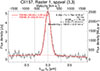 |
Fig. 1. Herschel PACS observation for NGC3393. Line broadening due to velocities up to 170 km s−1. |
 |
Fig. 2. Herschel PACS observation for NGC7603. Line broadening due to velocities up to 400 km s−1. |
The line profiles were broadened due to the superposition of many factors. The largest contribution to the widths is from the rotation of the disk of the galaxy because of the largest values of their velocities, although galactic outflows are also known Guillard et al. (2015).
It was necessary to apply a correction for the angle of inclination of the galactic disk to the line of sight, which was done using known formulas, assuming that galactic disk itself is resolved (Hubble 1926; Jacobs et al. 2009; Whittle 1992).
 (2)
(2)
Here, i is the inclination angle, (i = 0 for a galaxy seen face-on) a and b are the diameters of the projected ellipse, q0 = 0.2 is a good first approximation that is independent of the morphological type. After that, we obtained the real velocities by applying the correction
 (3)
(3)
Rotation velocities were estimated using the approximate formula
 (4)
(4)
where u, M, and R are the rotational speed, mass, and radius of the galaxy. Estimates based on reasonable values of the masses and radii of radiating media give rotational speed ranges of more than 200 km s−1. Indeed, for M = 1011 M⊙, R = 1 − 10 kpc, u = 655 − 207 km s−1, and for M = 5 ⋅ 1010 − 5 ⋅ 1011 M⊙, R = 1 − 10 kpc, u = 464 − 464 km s−1. It is clear that the presence of dark matter will only increase the values of the velocity estimates (Zotos & Caranicolas 2013). Thus, by selecting galaxies with observed linewidths corresponding to values less than 200 km s−1 (in our case), whose observed linewidths of the 158 μm [CII] line are broadened by reasons other than disk rotation (i.e., turbulence and velocity gradients of flows, which should also be turbulent because of large Reynolds numbers; see below), we obtained our sample with vrot < 200 km s−1. We chose values below 200 km s−1 in order to exclude rotational values, that is to include galaxies with linewidths broadened only by turbulence and small velocity gradients. Later, we also consider all galaxies (with all measured velocities).
In local star-forming galaxies, Croxall et al. (2017) have shown that 60–80% of the [CII] emission originates from neutral gas (HI clouds). In other words, because the size of the region emitting in the 158 μm [CII] line depends on the presence of CII ions, that is, on the ionization structure of the emitting medium, calculations of the corresponding structures become an important part of the quantitative description of turbulent media. The ionization structure of the nebula can be modeled (for example, by means of the Cloudy photoionization code), given the observational data in the Hα and Hβ lines and the concentration of the nebula. This will be presented in the forthcoming work.
3. Results and discussion: The amount of energy transferred in the cascade process of turbulent motions
The ISM of active galaxies, which is responsible for the radiation of emission lines, is in a complex kinematic state that is the result of a superposition of many flows caused by such phenomena as stellar and galactic winds, supernova remnants, and merging, all in the presence of a large number of turbulent eddies of different spatial scales. As is known, turbulence in a gaseous medium is associated with the emergence and development of a large number of vortex motions of various scales at certain velocities exceeding laminar values (Marov & Kolesnichenko 2013). For incompressible flows (ρ = const.; in the subsonic case, the approximation of incompressibility is good), in the Navier-Stokes equation,
 (5)
(5)
At any spatial scale, l, the advection term (u ⋅ ∇)u should be compared with the dissipation term ν∇2u to estimate their relative importance. The ratio of these terms gives the Reynolds number. The advection term can be approximated as  , and the dissipation term can be approximated as
  . Thus, the Reynolds number is given by
 (6)
(6)
Here ν is the kinematic viscosity for the density of the ISM, calculated for a concentration nH ∼ 100 cm−3, that is, for the density ρ ∼ 10−22 g cm−3, which gives ν = 3.5 ⋅ 1017 cm2 s−1 (Kaye & Laby 1995). Apart from this ν, an alternative estimate of kinematic viscosity under astrophysical conditions can also be made as follows (Lesaffre et al. 2020):
 (7)
(7)
where  is the mean free path for elastic (i.e., with conservation of energy and momentum) collisions of neutral hydrogen atoms and with the cross section σ ∼ 5.7 ⋅ 10−15 cm2 (Spitzer 1978), nH ∼ 100 cm−3, and cs ∼ 1 km s−1 at a temperature of T ∼ 100 K is the adiabatic speed of sound (Lesaffre et al. 2020). Thus, approximately, we again have ν ∼ 1.8 ⋅ 1017 cm2 s−1.
When the velocity of the moving medium exceeds the critical value given by the Reynolds threshold number, as is known, the flow becomes turbulent. Assuming that the characteristic size and characteristic velocity have the observed values l = lAG = 1021 cm and u = u(CII) ∼ 107 cm s−1 (Samsonyan 2022), we obtained the Reynolds number Re ∼ 1010, which is much greater than 104 (a threshold value for the incompressible flow to become completely turbulent). As already noted, all estimates and formulas regarding the cascade transfer of turbulent energy are applicable only to an incompressible flow, but numerical studies have shown that they can also be used for a compressible medium (Hattori et al. 1986).
Thus, in this case, the flow is undoubtedly turbulent (Marov & Kolesnichenko 2013). The transfer of kinetic energy on the characteristic scale lAG at the characteristic velocity ut in turbulent flows is given on average by a relation similar to (1) (in this case, multiplied by the density, in units of ergs per cubic centimeter per second. Marov & Kolesnichenko 2013; Godard et al. 2009). In Eq. (8) ut = urotr; that is, ut is equal to the real velocity. Also in Eq. (8), as mentioned above, lAG = 1021 cm, ut = 100 km s−1, and ρ = 10−22 g cm−3, which are typical for AG, so we obtain the given value of ϵ as
 (8)
(8)
This is about 8 ⋅ 10−23 erg cm−3 s−1.
The Kolmogorov scaling of turbulence processes postulates that the cascade energy transfer does not depend on the scale (Marov & Kolesnichenko 2013). This holds true in our Galaxy on scales between 0.01 and 1000 pc (Godard et al. 2009). On the other hand, in a highly compressible ISM, changes in the transmission rate are possible at different scales, but these deviations should not differ much from law (1), as mentioned above. We show that the same holds true for the medium of active galaxies that emit in the strongest lines, such as the [CII] 158 μm line.
The data suggest that the line broadening in our sample is related to the turbulent velocity (and also to flows with a velocity gradient, because they are turbulent due to a high Reynolds number), and the excitation of the medium is carried out by the turbulent energy injected by means of vortices of the maximum size lAG. This energy is further transferred in a cascade process and dissipated in the vortices of the smallest size, lmin, eventually turning into heat that excites atoms, ions, and molecules. This is determined, as mentioned above, by the mean free path of hydrogen atoms, with the cross section for elastic collisions σHH = 5.7 ⋅ 10−15 cm2. For comparison, the H2–H2 elastic collision cross section is σH2H2 ∼ 3 ⋅ 10−15 cm2 (Monchick & Schaefer 1980). At concentrations typical of the ISM in active galaxies, 100 cm−3 (Jaskot & Oey 2013), the dimensions of these vortices are lmin ∼ λMFP ∼ 1012 cm, that is, about 0.1 AU. As is mentioned above, the emission of [CII] comes from neutral HI clouds of kiloparsec scale, where on a small scale, the energy of turbulence is able to dissipate. That is, it is exactly at these small-scale eddies that excited atoms, ions, and molecules finally radiate energy, which may be observed, for example, in the [CII] 158 μm line. One can also estimate the dissipation time of the entire injected energy: tdiss = lAG/ut ∼ 106 − 107 years.
4. The luminosity of the active galaxies in the [CII] 158 μm line
We compare the observed luminosities with the total amount of turbulent energy transferred in cascade processes (reported in the Table A.1),
 (9)
(9)
where Eturb is amount of turbulent energy.
The observed luminosities of our galaxies in the [CII] 158 μm line are on the order of L ∼ 104 − 109 L⊙ = 4 ⋅ 1037 − 4 ⋅ 1042 erg s−1 Samsonyan (2022) and references therein). One may set k = 0.01–0.1 to account for various collisionally excited lines (e.g., low-lying fine-structure states of the ground energetic level) of different atoms, ions, and molecules in CII zone. For example, with n = 100 cm−3, lAG = 1 kpc, and ut ≈ 107 cm s−1, we obtained Eturb ≈ 1041 erg s−1, which is close to the observed values.
According to observations, the turbulent velocity dispersion of the molecular gas in active galaxies may be about 120 < σturb < 330 km s−1 (Guillard et al. 2015; Liang et al. 2024). By adjusting the parameters of the density, velocity, and sizes within appropriate limits, we obtained values close to the observed luminosities. Thus, the upper level of the total amount of turbulent energy for all such galaxies is close to that emitted in the [CII] 158 μm line (see Figs. 3, 4), or more precisely, it is several times greater, since possible radiation also occurs in other lines of other atoms, ions, or molecules. As one can see, there is a tendency for the observed luminosity in the line under consideration to increase with an increase in the amount of turbulent energy transferred in the cascade process.
 |
Fig. 3. Observed [CII] 158 μm luminosities (erg s−1) versus calculated turbulent energy rates (erg s−1) for galaxies with CII sizes of 1 kpc and concentration nH = 100 cm−3. |
Also noticeable in such diagrams (see Fig. 4) are the different behaviors of the SB and AGN galaxies, which is not surprising since it has been repeatedly reported that different degrees of excitation of various atoms, ions, and molecules depend on the conditions of the ISM, which are different in SB and AGN galaxies (Izumi et al. 2016). They are known as SB- and AGN-dominated galaxies, and the precise reasons for the observed difference are difficult to determine, though we may cautiously suggest a physical basis for the distinction. Turbulent motion, which likely dominates in SB galaxies, offers more degrees of freedom for energy dissipation compared to the more ordered motion associated with a velocity gradient, which may be more typical for AGN. Disentangling these effects will require extensive modeling efforts, including detailed ionization calculations that account for various ionization sources, the presence of dust, differences in the chemical abundances of elements and molecules, and the influence of magnetic fields. Furthermore, observations with a spatial resolution of parsecs or less are necessary to empirically distinguish between turbulent motion and flows with distinct velocity gradients.
Figure 5 displays the dependence of the observed luminosity of the 158 μm [CII] line on the degree of turbulent energy injection. In connection with Fig. 5, the following important circumstances should also be emphasized: A key feature of this plot is the distinct behavior of SB galaxies compared to AGN galaxies. This difference can be interpreted through the lens of classical turbulence theory (Kolmogorov cascade). Since the [CII] fine-structure line is excited by collisions with electrons, protons, hydrogen atoms, and molecules, theory implies that higher turbulence velocities should lead to increased energy dissipation and, consequently, higher emission in cooling lines such as [CII]. The SB galaxies are characterized by intense star formation, which drives high isotropic turbulence via supernova explosions and stellar winds. This results in high turbulence velocities (u) and a larger energy dissipation rate (u3/r), thereby increasing the energy available to excite the [CII] line. Conversely, AGN galaxies are dominated by central accretion activity, which induces shear flows rather than isotropic turbulence. Despite the presence of strong velocity gradients, shear flows in AGN may possess lower effective turbulence velocities or utilize different dissipation mechanisms, resulting in lower u3/r values compared to SB environments. The observed trends reveal interesting nuances. The shallower slope in SB galaxies suggests a nonlinear or less direct correlation between turbulent energy and emission, likely because other physical parameters–such as gas density, radiation field strength, or geometry–dominate the regulation of luminosity (Herrera-Camus et al. 2018). In contrast, the steeper slope in AGN indicates a more direct proportionality between turbulence energy input and [CII] luminosity, suggesting that confounding factors are less dominant. However, SB galaxies display a higher absolute luminosity despite this flatter slope. This points to supplementary heating mechanisms in SB regions (e.g., cosmic rays, UV radiation from massive stars, or shocks unrelated to turbulence) that augment [CII] emission beyond predictions based on turbulence alone. These results demonstrate that the enhancement of [CII] emission in large-scale turbulent, collisional environments is a critical factor for interpretation. (See also Herrera-Camus et al. 2015, 2018; Kaufman et al. 1999; Appleton et al. 2013; Fadda et al. 2023).
 |
Fig. 5. Luminosities of L(CII) versus E(turb) for different types of galaxies. Here, the different behavior of SB and AGN galaxies is evident. SB galaxies have a greater potential for dissipating turbulent energy, and therefore, the calculated luminosities tend to dominate those of AGN. The shallower slope in SB galaxies suggests a nonlinear or less direct correlation between turbulent energy and emission, likely because other physical parameters – such as gas density, radiation field strength, or geometry – dominate the regulation of luminosity. The slope of the dependence for AGN, on the other hand, is steeper, indicating a more direct proportionality between turbulence energy input and [CII] luminosity, suggesting that confounding factors are less dominant. |
Regarding the problem of the magnitude of turbulent velocity being on the order of the 600 km s−1, which we attribute in this work to the observed velocities, one can say that according to observations, typical turbulent velocity dispersions in SB molecular gas are 25–150 km s−1, and the highest values are observed in cases of high-velocity dispersion-disk SB galaxies with z ∼ 2, which also correlate with star formation rates (Green et al. 2010). The greater turbulence velocities in our sample may be driven by supernovae (Lacki 2013). To avoid misunderstandings, we also compared the results for galaxy samples with an upper velocity limit of 600 km s−1 (Fig. 5). It can be seen that the same trend is observed, that is, an increase in luminosity in the [CII] line occurs with an increase in the amount of turbulent energy transferred in the cascade process. Therefore, we think that all observed velocities are a combination of rotation, outflowing gas, and turbulence (Guillard et al. 2015) and that it is exactly the turbulence that is responsible for dissipation. Thus, excitation of turbulence with velocities of the order of rotation velocity should be inevitable because of differential rotation causing, for example, Kelvin-Helmholtz instability.
5. Conclusion
This paper is devoted to the influence of turbulent motions in the radiating medium of active galaxies on the widths of spectral lines. We considered the possibility of the redistribution of the turbulent energy of the ISM of active galaxies, excited by the activity of the nucleus (in the case of AGN) and by supernovae and stellar winds (in the case of SB galaxies), according to Kolmogorov’s theory. Turbulence in this environment is confirmed by the large value of the Reynolds number, about 1010. The medium is excited by large vortices, the scale of which is comparable to the characteristic size of the system. Further, the energy of these vortices is transformed into vortices of smaller scales, including down to vortices corresponding to the energy dissipation in vortices of the smallest size, with radii on the order of the mean free path of particles of the medium (about 1012 cm at the typical concentration of the ISM of active galaxies of about 100 cm−3). The energy is then radiated away. Quantitatively, this measure is determined by the cube of the velocity divided by the size of the radiating medium, which is supported by observations of galaxies in the CII 158 μm line. Moreover, the luminosity of galaxies in this line (about 1040 − 1042 erg s−1) is proportional to the amount of turbulent energy transferred in the Kolmogorov cascade process down to smaller vortices (Ėturb ≈ k(1040−1045) erg s−1 for such galaxies, where k is less than 1). Turbulence can be generated by many sources and even by a combination of them, but in this case of high turbulent speeds, it is most likely generated by the expansion of superbubbles and supernovae flows. AGN-driven galactic flows may also contribute (Norman & Ferrara 1996; Korpi et al. 1999; Dib et al. 2006; Joung & Mac Low 2006; Joung et al. 2009) because such flows all have a velocity gradient and should broaden the line profiles.
Acknowledgments
This work was made possible by a research grant number 21AG-1C044 from the Science Committee of the Ministry of Education, Science, Culture and Sports RA. Calculations were performed using the equipment of the AvH. We thank also Daniel W. Weedman for his invaluable suggestions. The authors thank the referee for careful reading and constructive suggestions, which have significantly improved the paper.
References
- Appleton, P. N., Guillard, P., Boulanger, F., et al. 2013, ApJ, 777, 66 [CrossRef] [Google Scholar]
- Croxall, K. V., Smith, J. D., Pellegrini, E., et al. 2017, ApJ, 845, 96 [Google Scholar]
- Dib, S., Bell, E., & Burkert, A. 2006, ApJ, 638, 797 [NASA ADS] [CrossRef] [Google Scholar]
- Fadda, D., Sutter, J. S., Minchin, R., & Polles, F. 2023, ApJ, 957, 83 [CrossRef] [Google Scholar]
- Godard, B., Falgarone, E., & Pineau Des Forêts, G. 2009, A&A, 495, 847 [NASA ADS] [CrossRef] [EDP Sciences] [Google Scholar]
- Green, A. W., Glazebrook, K., McGregor, P. J., et al. 2010, Nature, 467, 684 [NASA ADS] [CrossRef] [Google Scholar]
- Guillard, P., Boulanger, F., Lehnert, M. D., et al. 2015, A&A, 574, A32 [NASA ADS] [CrossRef] [EDP Sciences] [Google Scholar]
- Gurzadian, G. A. 1991, Ap&SS, 179, 293 [Google Scholar]
- Hattori, F., Takabe, H., & Mima, K. 1986, Phys. Fluids, 29, 1719 [Google Scholar]
- Herrera-Camus, R., Bolatto, A. D., Wolfire, M. G., et al. 2015, ApJ, 800, 1 [Google Scholar]
- Herrera-Camus, R., Sturm, E., Graciá-Carpio, J., et al. 2018, ApJ, 861, 95 [Google Scholar]
- Hubble, E. P. 1926, ApJ, 64, 321 [Google Scholar]
- Izumi, T., Kohno, K., Aalto, S., et al. 2016, ApJ, 818, 42 [NASA ADS] [CrossRef] [Google Scholar]
- Jacobs, B. A., Rizzi, L., Tully, R. B., et al. 2009, AJ, 138, 332 [NASA ADS] [CrossRef] [Google Scholar]
- Jaskot, A. E., & Oey, M. S. 2013, ApJ, 766, 91 [Google Scholar]
- Joung, M. K. R., & Mac Low, M.-M. 2006, ApJ, 653, 1266 [NASA ADS] [CrossRef] [Google Scholar]
- Joung, M. R., Mac Low, M.-M., & Bryan, G. L. 2009, ApJ, 704, 137 [NASA ADS] [CrossRef] [Google Scholar]
- Kaufman, M. J., Wolfire, M. G., Hollenbach, D. J., & Luhman, M. L. 1999, ApJ, 527, 795 [Google Scholar]
- Kaye, G., & Laby, T. 1995, Tables of Physical and Chemical Constants (London: Longman) [Google Scholar]
- Korpi, M. J., Brandenburg, A., Shukurov, A., Tuominen, I., & Nordlund, Å. 1999, ApJ, 514, L99 [NASA ADS] [CrossRef] [Google Scholar]
- Lacki, B. C. 2013, arXiv e-prints [arXiv:1308.5232] [Google Scholar]
- Lebouteiller, V., Cormier, D., Madden, S. C., et al. 2012, A&A, 548, A91 [NASA ADS] [CrossRef] [EDP Sciences] [Google Scholar]
- Lesaffre, P., Todorov, P., Levrier, F., et al. 2020, MNRAS, 495, 816 [NASA ADS] [CrossRef] [Google Scholar]
- Liang, L., Feldmann, R., Murray, N., et al. 2024, MNRAS, 528, 499 [NASA ADS] [CrossRef] [Google Scholar]
- Marov, M. Y., & Kolesnichenko, A. V. 2013, Turbulence and Self-Organization (Springer), 389 [Google Scholar]
- Monchick, L., & Schaefer, J. 1980, J. Chem. Phys., 73, 6153 [Google Scholar]
- Norman, C. A., & Ferrara, A. 1996, ApJ, 467, 280 [NASA ADS] [CrossRef] [Google Scholar]
- Samsonyan, A. L. 2022, Astrophysics, 65, 151 [NASA ADS] [CrossRef] [Google Scholar]
- Samsonyan, A., Weedman, D., Lebouteiller, V., Barry, D., & Sargsyan, L. 2016, ApJS, 226, 11 [Google Scholar]
- Spitzer, L. 1978, Physical Processes in the Interstellar Medium (A Wiley-Interscience Publication) [Google Scholar]
- Whittle, M. 1992, ApJS, 79, 49 [Google Scholar]
- Wilson, O. C., & Vainu Bappu, M. K. 1957, ApJ, 125, 661 [NASA ADS] [CrossRef] [Google Scholar]
- Zotos, E. E., & Caranicolas, N. D. 2013, A&A, 560, A110 [NASA ADS] [CrossRef] [EDP Sciences] [Google Scholar]
Appendix A: [C II] luminosities and turbulent energies
Observed L(CII) luminosities and calculated turbulent energies transferred down in the cascade processes.
All Tables
Observed L(CII) luminosities and calculated turbulent energies transferred down in the cascade processes.
All Figures
|
Fig. 1. Herschel PACS observation for NGC3393. Line broadening due to velocities up to 170 km s−1. |
| In the text | |
|
Fig. 2. Herschel PACS observation for NGC7603. Line broadening due to velocities up to 400 km s−1. |
| In the text | |
|
Fig. 3. Observed [CII] 158 μm luminosities (erg s−1) versus calculated turbulent energy rates (erg s−1) for galaxies with CII sizes of 1 kpc and concentration nH = 100 cm−3. |
| In the text | |
 |
Fig. 4. Same as Fig. 3, but for all galaxies in the sample. |
| In the text | |
|
Fig. 5. Luminosities of L(CII) versus E(turb) for different types of galaxies. Here, the different behavior of SB and AGN galaxies is evident. SB galaxies have a greater potential for dissipating turbulent energy, and therefore, the calculated luminosities tend to dominate those of AGN. The shallower slope in SB galaxies suggests a nonlinear or less direct correlation between turbulent energy and emission, likely because other physical parameters – such as gas density, radiation field strength, or geometry – dominate the regulation of luminosity. The slope of the dependence for AGN, on the other hand, is steeper, indicating a more direct proportionality between turbulence energy input and [CII] luminosity, suggesting that confounding factors are less dominant. |
| In the text | |
Current usage metrics show cumulative count of Article Views (full-text article views including HTML views, PDF and ePub downloads, according to the available data) and Abstracts Views on Vision4Press platform.
Data correspond to usage on the plateform after 2015. The current usage metrics is available 48-96 hours after online publication and is updated daily on week days.
Initial download of the metrics may take a while.