| Issue |
A&A
Volume 694, February 2025
|
|
|---|---|---|
| Article Number | A180 | |
| Number of page(s) | 12 | |
| Section | Astrophysical processes | |
| DOI | https://doi.org/10.1051/0004-6361/202451991 | |
| Published online | 11 February 2025 | |
The impact of mass uncertainties on r-process nucleosynthesis in neutron star mergers
Institut d’Astronomie et d’Astrophysique, Université Libre de Bruxelles (ULB), CP 226, B-1050 Brussels, Belgium
⋆ Corresponding author; This email address is being protected from spambots. You need JavaScript enabled to view it.
Received:
26
August
2024
Accepted:
20
December
2024
Abstract
Context. Theoretically predicted yields of elements created by the rapid neutron capture (r-) process carry potentially large uncertainties associated with incomplete knowledge of nuclear properties and approximative hydrodynamical modeling of the matter ejection processes. One of the dominant uncertainties in determining the ejecta composition and radioactive decay heat stems from the still unknown nuclear masses of exotic neutron-rich nuclei produced during the neutron irradiation.
Aims. We investigate both the model (systematic) and parameter (statistical) uncertainties affecting nuclear mass predictions and explore their impact on r-process production, and subsequently on the composition of neutron star merger ejecta.
Methods. The impact of correlated model uncertainties on masses is estimated by considering five different nuclear mass models that are known to provide an accurate description of known masses. In addition, the uncorrelated uncertainties associated with local variation of model parameters are estimated using a variant of the backward-forward Monte Carlo method, to constrain the parameter changes to experimentally known masses before propagating them consistently to the unknown masses of neutron-rich nuclei. The impact of nuclear mass uncertainties is propagated to r-process nucleosynthesis in a 1.38–1.38 M⊙ neutron star merger model considering a large and representative number of trajectories.
Results. We find that the uncorrelated parameter uncertainties lead to ejected abundance uncertainties of 20% up to A ≃ 130 and 40% between A = 150 and 200, with peaks around A ≃ 140 and A ≃ 203 giving rise to deviations around 100–300%. The correlated model uncertainties remain larger than the parameter ones for most nuclei. However, both model and parameter uncertainties have an important impact on heavy nuclei production.
Conclusions. Improvements to nuclear models are still crucial in reducing uncertainties in predictions related to r-process nucleosynthesis. Both correlated model uncertainties and coherently determining parameter uncertainties are key in the sensitivity analysis.
Key words: nuclear reactions / nucleosynthesis / abundances / stars: neutron
© The Authors 2025
 Open Access article, published by EDP Sciences, under the terms of the Creative Commons Attribution License (https://creativecommons.org/licenses/by/4.0), which permits unrestricted use, distribution, and reproduction in any medium, provided the original work is properly cited.
This article is published in open access under the Subscribe to Open model. This email address is being protected from spambots. You need JavaScript enabled to view it. to support open access publication.
1. Introduction
The r-process in stellar nucleosynthesis is essential for explaining the production of stable (and some long-lived radioactive) neutron-rich nuclides heavier than iron observed in stars of various metallicities, including in the Solar System (see reviews of Arnould et al. 2007; Arnould & Goriely 2020; Cowan et al. 2021).
Over the years, various nuclear-physics-based and astrophysics-free models of the r-process, varying in sophistication, have been developed. Advances in modeling type-II supernovae and γ-ray bursts have generated excitement around the neutrino-driven wind environment. However, achieving a successful r-process ab initio remains elusive without tuning relevant parameters (neutron excess, entropy, expansion timescale) in a manner not supported by the most sophisticated existing models (Janka 2017). While these scenarios hold promise, especially with their potential to contribute significantly to the Galactic enrichment, they are plagued by significant uncertainties, primarily stemming from the still incompletely understood mechanism behind supernova explosions and the persistent challenges in obtaining suitable r-process conditions in self-consistent dynamical explosion and neutron star (NS) cooling models (Janka 2017; Wanajo et al. 2018; Bollig et al. 2021). In particular, a subclass of core-collapse supernovae known as collapsars, and corresponding to the fate of rapidly rotating and highly magnetized massive stars, often considered as the origin of observed long γ-ray bursts, could emerge as a promising r-process site (Nishimura et al. 2015; Siegel et al. 2019; Just et al. 2022). The production of r-nuclides in these events may be associated with jets predicted to accompany the explosion or with the accretion disk forming around a newly born central black hole (BH).
Since the early 2000s, special attention has been directed toward NS mergers (NSMs) as potential r-process sites, especially after hydrodynamic simulations confirmed the ejection of a nonnegligible amount of matter from the system. Newtonian simulations, conformally flat general relativistic simulations, as well as fully relativistic hydrodynamical simulations involving NS-NS and NS-BH mergers with microphysical equations of state, have shown that, typically, a fraction ranging from 10−3 M⊙ up to more than 0.1 M⊙ can become gravitationally unbound on roughly dynamical timescales due to shock acceleration and tidal stripping. Additionally, the relic object, either a hot, transiently stable hypermassive NS followed by a stable supermassive NS, or a BH-torus system, can lose mass through outflows driven by various mechanisms (Just et al. 2015).
Increasingly sophisticated simulations have reinforced the idea that the ejecta from NSMs serve as viable r-process sites up to the third abundance peak (76 ≤ Z≤ 88) and the actinides (Z ≥ 89). The enrichment of r-nuclides is predicted to originate from both the dynamical (prompt) material expelled during the NS-NS or NS-BH merger phase and the outflows generated during the post-merger remnant evolution of the relic NS-torus and BH-torus system (Just et al. 2015, 2023). The resulting abundance distributions align closely with the Solar System distribution and various elemental patterns observed in low-metallicity stars (Cowan et al. 2021). Moreover, the ejected mass of r-process material, combined with the predicted astrophysical event rate (around 10 My−1 in the Milky Way), can account for the majority of r-material in our Galaxy (see for example Shen et al. 2015). Another compelling piece of evidence supporting NSMs as r-nuclide producers comes from the highly important gravitational-wave and electromagnetic observation of the kilonova GW170817 in 2017 (Abbott et al. 2017; Watson et al. 2019; Gillanders et al. 2022).
Despite recent successes in nucleosynthesis studies for NSMs, the details of r-processing in these events are still subject to various uncertainties, particularly in the nuclear physics input (see e.g., Mendoza-Temis et al. 2015; Kullmann et al. 2023). One of the dominant uncertainties stems from the still unknown nuclear masses of exotic neutron-rich nuclei produced during the neutron irradiation. Indeed, in typical NSM conditions, the high neutron density and high temperatures lead the nuclear flow to be essentially constrained by radiative neutron captures and photoneutron emissions. Despite the relatively wide literature on the impact of masses on r-process nucleosynthesis (see e.g., Goriely 2015; Mendoza-Temis et al. 2015; Sprouse et al. 2020; Mumpower et al. 2016; Kullmann et al. 2023), the propagation of mass uncertainties on the composition of the ejecta remains a complicated task, especially in view of the different types of correlation embedding differential quantities, such as the neutron separation (Sn) or β-decay (Qβ) energies.
In this paper, we study both nuclear model (or equivalently “systematic”) and nuclear parameter (often referred to as “statistical”) uncertainties affecting the prediction of theoretical masses. The aim is to coherently determine their impact on the composition of the ejecta of NSMs through their influence on the neutron-capture to photoneutron rate ratios.
Section 2 presents the method for obtaining model and parameter uncertainties, with a special emphasis on the application of the backward-forward Monte Carlo (BFMC) approach to constrain parameter uncertainties on experimental data. In Sect. 3 we study the impact of both the parameter and model uncertainties on r-process nucleosynthesis in a 1.38–1.38 M⊙ NSM simulation. Finally, in Sect. 4 we discuss the results of this work and the potential perspectives of this sensitivity study.
2. Method
This section outlines the methodology employed to assess uncertainties in nuclear mass models and their impact on critical nuclear parameters relevant to r-process nucleosynthesis. Understanding these uncertainties is essential for accurately predicting the behavior of nuclei far from stability and their role in astrophysical processes.
We first examined the uncertainties in various nuclear mass models and their accuracy in predicting masses of neutron-rich nuclei. Next, we used the BFMC method to quantify parameter uncertainties in neutron separation energies and β-decay energies. We then compared different methods for estimating these uncertainties and ensured consistency in predictions for neighboring nuclei. This methodology provides a foundation for analyzing how these uncertainties impact r-process nucleosynthesis predictions.
2.1. Nuclear model uncertainties
Many different mass models have been proposed so far. Such models can be characterized by very different frameworks, some of them based on the liquid-drop type of approach with additional microscopic corrections, others on the mean-field method using either relativistic or nonrelativistic energy density functionals (Lunney et al. 2003). Even within a given framework, different expressions are used to determine the various ingredients and corrections to the mass calculations (e.g., a volume or surface pairing interaction, inclusion of extra terms in the functional, coordinate or oscillator basis representation, ...). These different physical descriptions used to estimate the nuclear mass define the model uncertainties.
The model uncertainties are treated in a similar way to that done by Kullmann et al. (2023) by adopting different nuclear mass models that have proven their capacity to reproduce fairly accurately known masses, that is, typically with a global root-mean-square (rms) deviation with respect to all known experimental masses below 0.8 MeV. More specifically, we adopted six different mass models here, based on either the macroscopic-microscopic or the mean-field approach, namely the Skyrme-HFB model with BSkG3 interaction (hereafter BSkG3; Grams et al. 2023), Skyrme-HFB model with BSk24 interaction (hereafter HFB-24; Goriely et al. 2013), Gogny-HFB model with D1M interaction (hereafter D1M; Goriely et al. 2009a), Gogny-HFB model with the three-range D3G3M interaction (hereafter D3G3M; Batail et al. 2024), Weiszäker-Skyrme macroscopic-microscopic model (hereafter WS4; Wang et al. 2014), and Finite-range droplet macroscopic-microscopic model (hereafter FRDM12; Möller et al. 2016).
In order to best meet the nuclear physics needs of the r-process, we required the applied models to be accurate with respect to experimental observables but also as reliable as possible, that is, to be based on a physically sound model that is as close as possible to a microscopic description of the nuclear systems. The first criterion is an objective measure, while the latter criterion may be seen as more subjective, namely that nuclear models which are as close as possible to solving the nuclear many-body problem on the scale of the nuclear chart have a stronger predictive power. This second criterion is, however, fundamental for applications involving extrapolation away from experimentally known regions, in particular toward exotic neutron-rich nuclei of relevance for the r-process.
The abovementioned mass models all lead to a relatively accurate description of the experimental masses (Wang et al. 2021) for all the 2457 nuclei with Z and N larger than 8, and which are all characterized by an rms deviation typically below 0.8 MeV. However, this overall accuracy does not imply a reliable extrapolation far away from the experimentally known region, since models may achieve a small rms value by mathematically driven or unphysical corrections or can have possible shortcomings linked to the physics theory underlying the model. In particular, despite its great empirical success, the macroscopic-microscopic approach suffers from major shortcomings, such as the incoherent link between the macroscopic part and the microscopic correction, the instability of the mass prediction to different parameter sets, or the instability of the shell correction (Pearson 2001; Lunney et al. 2003). For this reason, microscopic mean-field mass models have been developed for the past two decades and are expected to provide more reliable predictions for r-process applications.
For the exotic neutron-rich nuclei relevant to the r-process, for which no experimental information is available, model uncertainties are shown to dominate over parameter uncertainties (Goriely & Capote 2014). By definition, the model uncertainties are correlated by the underlying model, so that their propagation into r-process nucleosynthesis calculation cannot be done through standard Monte Carlo-type approaches.
2.2. Nuclear parameter uncertainties
In contrast to model uncertainties describing the physical nature of the nuclear system, the parameter uncertainties are associated with local variations of the many parameters attached to a given model. Since none of the model is rooted in a parameter-free fundamental theory, model parameters are tuned to best reproduce experimental data. Even if such a fit leads to an optimum description of the relevant observables, local variation of these parameters may give rather similar reproduction of the data but still lead to nonnegligible differences when applied to unknown nuclei. These define the parameter uncertainties. In comparison with model uncertainties, much less effort has been devoted to estimating the parameter uncertainties affecting masses (Sprouse et al. 2020).
For this study, we considered the parameter uncertainties affecting one specific mass model: the Hartree-Fock-Bogolyubov (HFB) mass predictions, HFB-24 (Goriely et al. 2013), as studied in detail in Goriely & Capote (2014) within the BFMC framework. Each nuclear model has its own parameter uncertainties; however, constraining them is tedious work that needs a dedicated study (see Goriely & Capote 2014). In HFB-24, there are 30 model parameters, including 16 Skyrme, 5 pairing, 4 Wigner, and 5 collective parameters. In Goriely et al. (2013), each parameter was adjusted to optimize the prediction of the 2353 experimental masses of nuclei with N and Z ≥ 8 available in the 2012 Atomic Mass Evaluation (Audi 2012). In Goriely & Capote (2014), 21 of these 30 parameters (corresponding to the Skyrme and pairing interactions) were varied locally around the HFB-24 minimum in order to study their impact on the extrapolated mass, as explained below.
In the study of parameter uncertainties, the range of local variation for each parameter remains to be defined and is critical for estimating the magnitude of their impact on extrapolated masses. For this reason, it is fundamental that such local parameter variations be constrained as much as possible by available experimental data before being applied to unknown nuclei. In our case, we were able to estimate the impact of such parameter uncertainties on calculated rates by propagating them using Monte Carlo (MC) sampling constrained by available experimental masses (Wang et al. 2021). The method used here corresponds to the BFMC approach, as summarized below.
2.2.1. The concept of the BFMC method
The BFMC method (Chadwick et al. 2007; Bauge & Dossantos-Uzarralde 2011; Goriely & Capote 2014) relies on sampling of the model parameters and the use of a generalized χ2 estimator to quantify the likelihood of each simulation with respect to a given set of experimental constraints, here, the experimentally known masses (Wang et al. 2021).
The backward MC is used to select suitable parameter samples that agree with experimental constraints. In the BFMC method, the χ2 estimator is utilized to quantify a likelihood function that weights a given sample of {p1,...,pn} parameters when the Ne associated observables {σ1,...,σNe} closely match experimental data. Experimentally constrained masses are assumed to be independent. This assumption allowed us to use a χ2 criterion instead of a generalized weighting function. Thus, the weighting function is simply 1 when χ2 ≤ χcrit2, and 0 otherwise, where χcrit2 is a chosen critical value of χ2 (typically the rms deviation of the model with respect to experimental masses). We obtain from this backward step a subset of MC parameter combinations that are compatible with experimental constraints. Then, for the forward MC step, the selected subset of MC parameter combinations is applied to the calculation of the unmeasured quantities (here, the experimentally unknown masses).
2.2.2. Parameter uncertainties associated with HFB-24 masses
Parameter uncertainties associated with HFB-24 masses have been estimated using the BFMC method (Goriely & Capote 2014). At the end of the backward MC step, a subset of Ncombξ = 10931 combinations of parameters constrained by experimental masses (σM, exp ≤ 0.8 MeV) was obtained. For the forward MC step, this selected set of MC parameter combinations was applied to the calculation of the ∼5000 unknown masses of neutron-rich nuclei. By definition, this method yields uncorrelated uncertainties. It should be kept in mind that the results obtained by Goriely & Capote (2014) assume that the deformation energy is not affected by local parameter changes. Even if larger uncertainties could not be excluded for strongly deformed nuclei, such results are exact for spherical nuclei and in particular for those lying close to the neutron shell closures of particular interest for r-process applications.
In Goriely & Capote (2014), the uncertainties associated with such local changes of the HFB parameters were found to remain smaller than those associated with nonlocal changes described by the 27 different HFB mass models. It should, however, be kept in mind that for each mass model considered, uncertainties due to the parameter variations should also be applied and that if the model uncertainties are correlated by the underlying model, the parameter uncertainties remain uncorrelated. In the present work, the parameter uncertainties are considered only for the HFB-24 mass model.
2.3. Approaches to determining nuclear parameter uncertainties on Sn and Qβ
In this section we present four possible ways of determining, from the mass parameter uncertainties, the uncertainties affecting Sn and Qβ values of interest to r-process nucleosynthesis. The separation energy, Sn, of a (Z,N) nucleus, defined as
 (1)
(1)
where M is the atomic mass (estimated from the nuclear mass by including the masses of the electrons and their binding energies; Lunney et al. 2003) and mneut the neutron mass, plays a key role during r-process neutron irradiation by setting the most abundant nuclei produced within an isotopic chain due to the (n, γ)⇌(γ, n) competition (or, potentially, equilibrium) (Goriely & Arnould 1992). Additionally, Qβ, defined as
 (2)
(2)
is an important quantity affecting the energy production, but also the β-decay rates, and therefore the composition of the ejecta. The different approaches take into account various physical considerations that impact the overall estimation of the uncertainties, in particular the correlations inherent to mass differences.
Additionally, we stress that, to propagate nuclear uncertainties into astrophysical observables (Sect. 3), a procedure similar to the one detailed in Martinet et al. (2024) was followed here. This procedure is based on the propagation of a random choice of minimum and maximum values of Sn for all nuclei of interest during r-process irradiation, instead of a random choice between these minimum and maximum values. Such a procedure allows us to save computer time and still provides upper and lower values of astrophysical observables, such as the ejecta composition from NSMs, that do directly depend on Sn values.
To estimate the parameter uncertainties affecting the neutron separation energy, Sn, we first considered two possible approaches (Case 1 and 2). Case 1 (Sect. 2.3.1) applies the BFMC method to estimate the mass uncertainties, σM, of all unknown nuclei and uses Eq. (1) to propagate those to Sn. In contrast, Case 2 (Sect. 2.3.2) applies the BFMC method directly to Sn, that is, both masses defining Sn values are calculated coherently with the same parameter set selected by the BFMC method. Both cases are detailed below.
2.3.1. Case 1: Sn from uncorrelated BFMC masses
Figure 1 shows the uncorrelated mass uncertainties we deduce from the BFMC method (Goriely & Capote 2014). The nuclei outlined in magenta are the ∼2500 experimentally known masses. From the BFMC method (see Sect. 2.2.1), we expect the uncertainties for these nuclei to be of the order of the rms deviation of HFB-24 with respect to experimental masses, that is, 0.55 MeV. By extension, the neighboring unknown masses have uncertainties of the same magnitude. Indeed, the combination of parameters compatible with experimental uncertainties is not expected to induce large differences for neighboring nuclei, but to steadily increase when straying farther away from the experimentally known nuclei. This effect is clearly seen in Fig. 1, where the largest uncertainties, reaching values up to σM ≃ 3 MeV, are found in neutron-rich nuclei close to the neutron drip line. In turn, these uncorrelated mass uncertainties, σM, can be used to estimate the corresponding neutron separation energies (Eq. (1)) with their uncertainties, as illustrated in Fig. A.1, and define our Case 1.
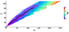 |
Fig. 1. Case 1: Representation in the (N,Z) plane of the uncorrelated masses uncertainties, σM(Z, N) (in MeV), obtained from 10931 runs with σM,exp < 0.8 MeV. See Goriely & Capote (2014) for more details. The nuclei outlined with open magenta squares are the experimentally known masses. The dashed magenta line is a contour of nuclei with σM below 0.55 MeV. The shell closures are displayed as plain lines. |
2.3.2. Case 2: Uncorrelated Sn from the BFMC method
The BFMC method applied to the masses was this time used for the neutron separation energy by computing Sn for each parameter combination and then discarding those incompatible with experimental data (i.e., only combinations with σM, exp < 0.8 MeV were retained). This approach assumes that each Sn, that is, masses of both (Z, N) and (Z, N − 1), is calculated with the same parameter set. In this way, we obtained a second case for our parameter uncertainties, based upon uncorrelated separation energies obtained directly from the BFMC method, composed of a subset of Ncombξ = 10643 combinations (sets of combinations were excluded on the basis of the Sn rms).
Figure 2 shows the resulting Sn uncertainties, σSn(Z, N). In contrast to Case 1, the uncertainties are distributed nonuniformly. Indeed, two features can be seen here. First, low uncertainties in Sn are found around each of the neutron magic numbers and uncertainties increase when straying farther away from these areas. Second, the uncertainties increase globally when going from low to high Z and from low to high N nuclei.
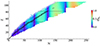 |
Fig. 2. Same as Fig. 1 but for Case 2: Uncorrelated Sn uncertainties (in MeV) determined in Case 2 within the BFMC method. |
The first feature is due to the separation energy being the difference between two neighboring masses. A low uncertainty shows that the local variation of the nuclear model parameters does not lead to a large difference between two neighboring nuclei. Around the magic numbers (N = 8, 20, 28, 50, 82, 126, and 184), a low uncertainty is found due to the conservation of the shell effects. When straying farther away from the magic numbers, the uncertainty increases, especially for neutron-rich nuclei.
Figure A.1 compares the separation energies for each isotopic chain from Z = 21 to Z = 100 obtained with Cases 1 and 2. The range of Sn obtained by the uncorrelated mass uncertainties from Case 1 is depicted in blue, while the uncorrelated Sn uncertainties from Case 2 are shown in red. For Case 1, we can clearly see the increase in the uncertainties as we go to neutron-rich nuclei. This effect increases with increasing N and Z. In particular, the uncertainties increase even more after the shell closures. If we look at Case 2, we see smaller uncertainties and a very mild increase in the overall uncertainties as we go to higher Z. It is interesting to note that Case 2 uncertainties around the neutron magic numbers are smaller than anywhere else along the isotopic chain. Moreover, we can observe that the uncertainties after the shell closures do not increase significantly, in contrast to what is found in Case 1.
Figure 3 shows the rms values of Sn and Qβ when choosing randomly for each nucleus a mass obtained from a random parameter set out of the 10931 BFMC combinations for Case 1 and of the 10643 BFMC combinations for Case 2. We repeated this procedure 200 times to obtain an average value of the dispersion. For Case 1 (blue curves), masses were randomly picked within the mass uncertainty, σM(Z, N), to compute the corresponding Sn and Qβ. The HFB-24 rms deviation with respect to experimental Sn amounts to 0.48 MeV and the one with respect to experimental Qβ to 0.59 MeV, as depicted by the dashed gray lines in Fig. 3. Although all combinations obtained with the BFMC method lead to rms deviations on experimental masses smaller than 0.8 MeV, the uncorrelated Sn and Qβ of Case 1 are seen to give rise to rms values significantly higher than those obtained by the HFB-24 mass model. This test clearly shows that the Sn and Qβ values deduced from uncorrelated masses are not properly constrained by experimental Sn and Qβ values, nor equivalently by the underlying correlations given by Eqs. (1–2).
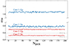 |
Fig. 3. rms values of Sn and Qβ when randomly picked Npick times from Case 1 or Case 2. The rms deviation is calculated with respect to all experimentally known Sn or Qβ values (Wang et al. 2021). The random pickup was done 200 times to obtain an average rms value. |
To understand such differences for Case 1, Fig. 4 shows the two-neutron separation energy, S2n, for one isotopic chain (here, Z = 70), using the same 200 random combinations discussed in Fig. 3. A much larger dispersion of S2n can be observed for Case 1 in comparison with Case 2. The important feature is highlighted in the insert, where we can see that while a clear shell gap at N = 126 is maintained for all combinations of Case 2, a potential disappearance of this shell effect is found for some combinations of Case 1, as highlighted by the thick blue line. The shell gap at neutron magic numbers is a well-known physical effect, so parameter combinations that would lead to the artificial disappearance of these shell effects need to be questioned.
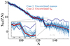 |
Fig. 4. Two-neutron separation energy, S2n, for the Z = 70 isotopic chain obtained with 200 combinations for Case 1 (blue lines) and 200 for Case 2 (red lines). A zoom on the N = 126 shell gap shows its potential disappearance in Case 1, a clear sign of overestimating the uncertainties in this case. One specific extreme combination of Case 1, shown by the thick blue line, highlights the possible shell disappearance. |
Such a feature found for most isotopic chains, combined with Fig. 3, underlines the overestimation of parameter uncertainties when estimating Sn from uncorrelated masses (Case 1). For this reason, we advise that Case 1 should not be used to estimate parameter uncertainties affecting Sn. Case 2 considers such correlations, but may underestimate the uncertainties, since the calculations of both associated masses are undertaken with the same parameter set. Anticorrelation between neighboring Sn values may also not be guaranteed in Case 2. In addition, a given set of Sn values may not correspond to one unique consistent set of masses. Both these issues to further improve Case 2 are tackled below with Cases 3 and 4, respectively.
2.3.3. Case 3: Anticorrelation between Sn
The neutron separation energy, by definition (Eq. (1)), links the atomic mass M(Z, N) to the mass of the neighbor nucleus M(Z, N − 1). Figure 5 shows the density heat map of the parameter uncertainties of the separation energy of a (Z,N) nucleus obtained in Case 2 as a function of the uncertainties affecting the (Z,N − 1) one for Z = 30 to Z = 101 isotopic chains. As can be seen for all isotopic chains, an anticorrelation is clear between two neighboring Sn. This comes from the fact that neighboring Sn are linked by the uncertainty of the mass of one of the two nuclei. A maximum uncertainty on Sn(Z, N) imposes a minimum (Z,N) mass or a maximum (Z,N-1) mass. This in turn will result in the Sn(Z, N − 1) being minimal.
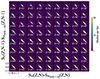 |
Fig. 5. Heat map representing the parameter uncertainty of Sn(Z, N − 1) (relative to HFB-24 values) as a function of Sn(Z, N) uncertainties (relative to HFB-24 values) for each BFMC combination selected in Case 2 (10643 combinations). The subplots use the same axis and are separated by isotopic chains to show the correlation for each of them. Each frame is 500 per 500 bins and each bin is color-coded to the number of combinations in it. |
To take this anticorrelation into account, we constructed Case 3 from Case 2, for which we imposed that each even-NSn(Z, N) be anticorrelated to its (Z,N − 1) neighboring value. In such conditions, we ensured that parameter uncertainties for (Z,N − 1) were coherent with its (Z,N) neighbor.
One of the main caveats of Case 3 is that, by keeping a random pick of the uncertainties for the even-N nuclei and imposing anticorrelation with their odd-N (Z,N − 1) neighbor nuclei only, it is possible that different masses are used for the same nucleus.
2.3.4. Case 4: Determining uncertainties of Sn and Qβ with consistent masses
To remedy the incoherent approach underlying Case 3 we then considered a Case 4 where we ensured that the neutron separation energies obtained with Case 2 not only led to anticorrelation between neighboring nuclei, but also that each set of Sn corresponded to a coherent set of masses. In addition, Case 4 included not only Sn but also Qβ as the main quantities to be minimized or maximized in the uncertainty analysis and their propagation.
In the same way as discussed for neighboring Sn values, Qβ(Z, N) given by Eq. (2) should be anticorrelated with Qβ(Z + 1, N − 1). Moreover, since Sn(Z, N) and Qβ(Z, N) are linked by the same (Z,N) mass, they should also be anticorrelated. Similarly to the results shown in Fig. 5, the density heat map of the parameter uncertainties of Qβ(Z + 1, N − 1) versus those of Qβ(Z, N) presents the same behavior. The anticorrelation also propagates along the isobaric chain, correlating the uncertainties of each nucleus composing it. Similar density heat maps are also found for the anticorrelation between Qβ(Z, N) and Sn(Z, N) uncertainties.
In Fig. 6, we show how imposing these three anticorrelations can result in imposing the choice of the masses throughout the whole nuclear network. For example, on the one hand, maximizing Sn(Z, N) is equivalent to choosing the minimum M(Z, N) and the maximum M(Z, N − 1) (see Eq. (1)). On the other hand, to maximize Qβ(Z, N) is equivalent to choosing the maximum M(Z, N) and the minimum M(Z + 1, N − 1). This leads to an anticorrelation between Sn and Qβ, where Qβ will be minimum when Sn is maximum, and vice versa. As depicted in Fig. 6, there will then be two resulting combinations of masses that will either maximize or minimize Sn and Qβ, with either all maximum masses on even-N nuclei and minimum on odd-N, or the opposite. In the end, we obtain two times two combinations, as we can either start maximizing or minimizing from the first even nuclei and propagate the coherent masses on the isotopic chain or we can do the same starting with the first odd nucleus. Note that another potential case could be obtained following a similar methodology but through Qβ along the isobaric chains.
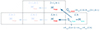 |
Fig. 6. Schematic view of the anticorrelations imposed by Sn and Qβ on the choices of mass uncertainties. When maximizing Sn(Z,N), we imposed Mmin(Z,N). The consequences of this choice are depicted in red, where the mass of (Z,N − 1) will need to be minimum and the mass of (Z+1,N − 1) maximum, due to the anticorrelation with Qβ. |
To compute these coherent Sn for Case 4, we needed to find the mass of (Z, N − 1) such that it maximized Sn(Z, N) keeping a coherent set of masses for the entire network. We were able to derive the coherent mass of (Z, N − 1) by extracting an associated uncertainty σM*(Z, N − 1) from Eq. (1). In the case where Sn(Z, N) is maximized, σM*(Z, N − 1) reads
 (3)
(3)
where σM(Z, N) and σSn(Z, N) are the uncorrelated mass and Sn uncertainties from the BFMC method, respectively (as extracted in Cases 1 and 2). Similarly, using Eq. (2), a new uncertainty for M(Z + 1, N − 1) can be obtained by minimizing Qβ and reads
 (4)
(4)
where σQβ(Z, N) is the uncorrelated Qβ uncertainty from the BFMC method (determined in a similar way to Case 2 for Sn). By deriving all the upper and lower limits of the masses for the network in this way, we were able to compute the corresponding Sn with the assurance that both anticorrelations in Sn and Qβ and a coherent set of masses were taken into account. This approach defined our Case 4 and the corresponding four combinations of anticorrelated minima and maxima in the neutron separation energies.
3. Impact on r-process nucleosynthesis
3.1. NSM simulations
We considered here the hydrodynamical simulation of a symmetric 1.38–1.38 M⊙ binary NS system and its postprocessing nucleosynthesis (Just et al. 2023). The simulation consistently included the dynamical component, the NS-torus transient, and the BH-torus remnant, in one unique long-term end-to-end evolution model (up to 100 s) with intermediate remnant lifetimes (between ∼0.1 − 1 s). The model considered here corresponds to the symmetrical simulation sym-n1a6 of Just et al. (2023).
We note that the nucleosynthesis abundances were calculated using a smaller representative subset of trajectories to reduce the computational demand. The subset of trajectories was chosen in such a way that it contained 10% of the total mass (as discussed in Kullmann et al. 2023) while still satisfactorily reproducing the properties (i.e., mass fraction distributions and heating rates) of the complete trajectory set. As a result, all calculations concerning the sym-n1a6 model included 358 trajectories.
The nucleosynthesis was followed by a reaction network consisting of ∼5000 species (depending on the set of nuclear masses adopted), ranging from proton numbers Z = 1 to Z = 100 and including all isotopes from the valley of β-stability to the neutron drip line. Elements with Z > 100 were assumed to fission spontaneously with very short lifetimes, since their production was found to be insignificant for the conditions found in the sym-n1a6 hydrodynamical model (Just et al. 2023) and in view of the HFB-14 fission barriers (Goriely et al. 2007; Goriely 2015; Lemaître et al. 2021; Kullmann et al. 2023) adopted in our present calculations. We note that the impact of this upper Z limit has been tested and is found to be negligible, while significantly reducing the CPU time. All reactions and decay modes of relevance, that is, neutron, proton, and α-capture reactions, photodisintegrations, β-decays, β-delayed processes, and α-decays are included. If the network reached trans-Pb species, we also included neutron-induced, spontaneous, and β-delayed fission and their corresponding fission fragment distributions for all nuclei. Each fissioning parent is linked to the daughter nucleus, and the emitted neutrons may be recaptured by the nuclei present in the environment.
Whenever experimental reaction or decay data were available, they were included in the network and were taken from the NETGEN1 library (Xu et al. 2013), which includes the latest compilations of experimentally determined rates. Whenever experimental reaction model ingredients (such as masses, energies, spin, and parities of ground and excited states) were available, they were also considered in the theoretical modeling. In this case, they also constrained the possible range of variation of the model parameters and reduced the impact on the model as well as parameter uncertainties. The model uncertainties affecting theoretical nuclear masses were propagated to the calculation of the radiative neutron capture and photoneutron rates. However, in the case of parameter uncertainties, the same radiative neutron capture rates as obtained on the basis of the HFB-24 mass model were calculated, and only the photoneutron rates were estimated on the basis of the modified neutron separation energies, Sn. Newly calculated rates were then consistently applied to the nucleosynthesis simulations to estimate their impact on r-process yields. Note that the uncertainties affecting masses were propagated into the Qβ values, which therefore may affect the decay heat, but not into the β-decay rates. Their impact on the abundance distribution is found to be relatively small with respect to those stemming from changes in the neutron separation energies.
To explore the impact of the correlated model and uncorrelated parameter uncertainties, a large number of nucleosynthesis calculations were performed, as described below.
3.2. Propagating parameter uncertainties
To propagate the uncorrelated parameter uncertainties, a large number, N, of sets containing randomly chosen minimum and maximum rates for each of the thousands of HFB-24 masses was produced. These were based on the maximum and minimum masses or Sn obtained in Sect. 2.2.1 from the BFMC method and one of the four cases described in Sect. 2.3. These random nuclear sets were then used in our NSM model to assess the impact of the parameter uncertainties on the final composition of ejecta.
One of the difficulties with randomly produced sets of masses or Sn is ensuring that enough draws have been made to be representative of the full range of possible outcomes. We computed an increasing number of simulations until convergence of the upper and lower limits of the ejecta abundances was reached. More specifically, the convergence was evaluated by the quantity
 (5)
(5)
where NA is the total number of nuclides and
![Mathematical equation: $$ \begin{aligned} \Delta _N = \mathrm{max}[\log (X)] - \mathrm{min}[\log (X)], \end{aligned} $$](/articles/aa/full_html/2025/02/aa51991-24/aa51991-24-eq6.gif) (6)
(6)
where X is the mass fraction and N is the number of r-process simulations considered (up to 50).
Figure 7 shows the convergence of the averaged uncertainties,  , as a function of the number, N, of simulations for our four cases. For small values of N, a rapid increase is expected due to the random nature of the draws, leading to large variations in the uncertainties. For more than typically N = 20 simulations, a plateau is found and the global abundance uncertainty does not evolve any more when compared to the value for N = 40 simulations. Hence, we consider that we convincingly converge to the total propagation of parameter uncertainties by computing N ≥ 20 stellar simulations with as many different nuclear masses, Sn, or anticorrelated Sn sets. Case 4 is, per construction, a set made of four combinations and is just indicated for completeness.
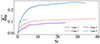 |
Fig. 7. Convergence of the averaged uncertainties, |

3.3. Case 1 vs. Case 2: Uncorrelated masses vs. uncorrelated Sn
Figure 8 shows the propagated nuclear uncertainties to the final abundances of our NSM model. The solar r-abundances are depicted in gray as a reference and scaled to the peak value of the A = 130 abundance given by the Case 1 simulation. Since an (n,γ)–(γ,n) equilibrium is established in most of the ejecta trajectories, masses play a key role in defining where such an equilibrium is achieved in each isotopic chain. As expected from Sect. 2.3.2, the propagation of larger Sn uncertainties, especially for neutron-rich nuclei, leads to larger uncertainties in r-process production. For the elements up to Ni, their production mostly happens in trajectories with a relatively high electron fraction, Ye ≳ 0.4 (Just et al. 2023). For this reason, the nucleosynthesis of A ≲ 70 nuclei is not significantly affected by mass uncertainties. In contrast, heavier species are produced by low Ye trajectories which include the production of exotic neutron-rich nuclei for which mass uncertainties are large, in particular if obtained within Case 1. Large deviations are found in particular for A > 140 mass fractions in Case 1. Such deviations are already significantly reduced when adopting Case 2 uncertainties. It is important to note that Case 2 is not just a subset of Case 1. For this reason, some abundances found within Case 2 cannot be obtained within Case 1, for example, around A ≃ 210. The possible disappearance of the N = 126 shell closure in the overestimated uncertainties of Case 1 is translated into a third r-process peak that is either flattened or reduced.
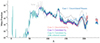 |
Fig. 8. Impact of the nuclear mass uncertainties obtained in Cases 1 to 4 on the mass fractions of stable nuclei (and long-lived Th and U) of the material ejected from the binary 1.38–1.38 M⊙ NSM model as a function of the atomic mass, A. Solar r-abundances (Goriely 1999) are shown in gray as a reference and are scaled to the peak value of the A = 130 abundance in the Case 1 simulation. |
3.4. Case 3: Correlated Sn
Sect. 2.3.4 discussed the anticorrelation existing between the separation energy, Sn, of the (Z,N) nucleus and its (Z,N − 1) neighbor. To take this anticorrelation into account, we then drew only randomly the maximum or minimum uncertainty for the even nuclei and imposed that the Sn uncertainty of its (Z,N − 1) neighbor took the opposite sign (i.e., minimum or maximum uncertainty, respectively). Figure 8 compares Case 3 against Cases 1 and 2. As expected, the anticorrelation forces fewer combinations, which also leads to reduced uncertainties for the r-process abundances. This effect becomes important for A > 150, especially for actinide production. The discrepancy between Cases 2 and 3 shows that, above A = 205, some extreme abundances can only be obtained for specific combinations. It underlines that the masses are highly sensitive to nuclear uncertainties in this range and very specific combinations of the uncertainties can lead to major differences in the nucleosynthesis predictions.
3.5. Case 4: Correlated Sn and coherent masses
To tackle the incoherent approach underlying Case 3, we then considered Case 4, where we ensured that each set of Sn corresponded to a consistent set of masses (see Sect. 2.3.4), and included not only Sn but also Qβ as the main quantities to be minimized or maximized in the uncertainty analysis and their propagation. The resulting abundance uncertainties of Case 4 shown in Fig.8 are slightly smaller than for Case 3 and lead to slightly different values. However, the feature of a small production of Pb and actinides remains.
3.6. Summary of the four cases
Figure 9 shows the abundance uncertainties (given by the ratio of maximum to minimum mass fractions) stemming from nuclear mass uncertainties, as described by our four cases. As discussed in Sect. 2.3.1, Case 1 systematically overestimates uncertainties, in particular in the vicinity of shell closures, and should be avoided in estimating nuclear mass uncertainties. Alternatively, Case 2, while being a more reasonable estimate, remains nonphysical since the anticorrelation between neighboring Sn or Qβ values is neglected. This anticorrelation is remedied by Case 3, but with the drawback that Sn values may not correspond to one unique and coherent set of masses. For these reasons, both Case 2 and Case 3 should not be used to estimate and propagate nuclear uncertainties. Finally, Case 4 represents our recommended estimate of parameter uncertainties, as it fulfills all the above physical requirements. After propagation, with Case 4 we find abundance uncertainties ranging between factors of 1.5 and 3, while Case 1 leads to deviation ranging from a factor of 3 to more than 10 (see Fig. 9).
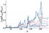 |
Fig. 9. NSM abundance uncertainties (in log scale) given by the ratio of maximum to minimum mass fractions (Xmax/Xmin) resulting from Sn uncertainties, as obtained in Cases 1 to 4. |
3.7. Systematic vs. statistical uncertainties
Fig. 10 compares the impact of the parameter uncertainties affecting the HFB-24 mass model (within the Case 4 approach) with the impact of model uncertainties for which the six different mass models described in Sect. 2.1 are adopted, namely two macroscopic-microscopic models, WS4 (Wang et al. 2014), and FRDM12 (Möller et al. 2016), and four mean-field models, HFB-24 (Goriely et al. 2013), BSkG3 (Grams et al. 2023), D1M (Goriely et al. 2009b), and D3G3M (Batail et al. 2024). It should be recalled that each mass model has its own parameter uncertainties that should be assessed using the same methodology, as detailed in the present study. We can see that the final composition of the NSM ejecta is less affected by the HFB-24 parameter uncertainty in comparison to the impact the model uncertainties can have. For A ≳ 203, the parameter uncertainties may, however, become more significant than the model ones.
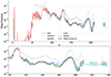 |
Fig. 10. Same as Fig. 8 but for the impact of model vs. parameter mass uncertainties. The six nuclear models used here are described in Sect. 2.1. The insert zoomed in the lower panel shows the A > 120 range where r-process nucleosynthesis is dominantly impacted by the parameter and model uncertainties. The blue-shaded range gives the HFB-24 associated parameter uncertainties. |
Figure 11 compares the maximum-to-minimum abundance ratios obtained with Case 4 uncorrelated parameter uncertainties and those obtained from model uncertainties. It should be stressed that model uncertainties are correlated by the model (see discussion in Martinet et al. 2024). In this case, the upper and lower limits should not be seen as a possible band defining minimum or maximum abundances. Comparing them to Case 4 parameter uncertainties (that are uncorrelated), we can see a clear overestimate of the uncertainties when misinterpreting the correlation underlying model uncertainties. The peak of Case 4 uncertainties around A ≃ 140, combined with the high uncertainty among models, underlines a large sensitivity of the predicted abundances with respect to remaining parameter uncertainties. Interestingly, the parameter uncertainty at A ≃ 202 is higher than the model uncertainty, also stressing a high sensitivity with respect to parameter uncertainties.
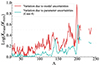 |
Fig. 11. Abundance uncertainties (Xmax/Xmin) for Case 4 vs. model uncertainties (using WS4, D1M, FRDM12, BSkG3, D3G3M, and HFB-24 models). Here, the model uncertainties are represented as if they would be uncorrelated, a common misrepresentation of the correlated model uncertainties (Martinet et al. 2024). |
3.8. Propagation of mass uncertainties on neutron capture rates and r-process abundances
Thus far, we had not propagated the mass uncertainties to the neutron capture rates themselves due to the heavy computation time this entails. However, in Case 4 specifically, the number of combinations is small and the calculation of reaction rates feasible. The neutron capture rates in Case 4 mass uncertainties were consequently calculated coherently using the TALYS reaction code (Koning et al. 2023) with the associated masses. These uncertainties were then propagated to r-process nucleosynthesis simulations together with masses for the calculation of photo rates.
Figure 12 shows the ratio of the maximum to minimum neutron capture rates resulting from the propagation of nuclear mass uncertainties of Case 4. Experimental masses are used whenever available, so that for those nuclei around the valley of stability no uncertainty associated with theoretical masses exists. However, straying farther away from the stability results in large uncertainties on the neutron capture rates, with up to a 103 ratio between the maximum and minimum rates. Small uncertainties are found around magic numbers for the reasons discussed in Fig. 2.
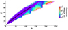 |
Fig. 12. Neutron capture rate uncertainties obtained from TALYS computations using Case 4 mass uncertainties. The reactions are color-coded by their parameter uncertainties (the ratio between maximum and minimum rates). |
Figure 13 displays the final abundance uncertainties resulting from the Case 4 nuclear mass uncertainties, taking or not taking into account the propagation to neutron capture rates. The abundance uncertainties are found to be almost identical, with or without a coherent calculation of the neutron capture rates due to the fairly well-established (n, γ)−(γ, n) equilibrium in the specific NSM model considered here. A slightly larger uncertainty for heavy nuclei production above A ≳ 200 is obtained, though, when including the propagation to (n, γ) rates. This test shows that our previous results, obtained by propagating the nuclear mass uncertainties without coherently computing the neutron capture rates, are a good first-order approximation.
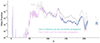 |
Fig. 13. Abundance uncertainties for Case 4 with and without propagation of the mass uncertainties to Hauser-Feshbach computations of neutron capture rates. |
4. Conclusions
We investigated both the model (systematic) and parameter (statistical) uncertainties associated with theoretical masses and their correlated neutron separation energies and Qβ values relevant for r-process nucleosynthesis. We considered six mass models to estimate the correlated model uncertainties and, for one model, namely HFB-24, we applied the BFMC approach to anchor the parameter uncertainties with available experimental data, that is, the known masses. In doing so, we obtain for HFB-24 an estimate of the upper and lower limits to the 5000 unknown masses involved in the r-process network. We explored four cases to propagate the mass uncertainties into the neutron separation energies, taking into account various physical considerations. Correlated model uncertainties are overall larger than uncorrelated parameter uncertainties, but both can differ significantly for the neutron-rich nuclei involved in the r-process.
We determined the impact of these nuclear uncertainties on r-process nucleosynthesis in a 1.38–1.38 M⊙ symmetrical NSM model (from Just et al. 2023), taking into account the production in the dynamical component, the NS-torus transient, and the subsequent BH-torus remnant. We considered nucleosynthesis calculation for the 358 trajectories representative of the overall ejecta. Around 40 models were computed for each case, using combinations of maximum and minimum nuclear masses or Sn in order to propagate the parameter uncertainties to the r-process abundances.
We find that using the uncorrelated mass uncertainties leads to a systematic overestimate of the final abundance uncertainties. Using the neutron separation energy, the key quantity defining the r-process path, results in a much better constraint on the uncertainties. However, special attention has to be paid to taking the anticorrelation with the isotopic neighbor into account. The anticorrelation existing between Qβ and Sn also needs to be taken into account. We finally obtain a coherent estimate of the uncertainties in our Case 4, taking into account these physical requirements. For this chosen case, we obtain r-process abundance uncertainties of the order of 20% up to A ≃ 130, 40% between A = 150 and 200, and peaks around A ≃ 140 and A ≃ 203 giving rise to deviations around 100 to 300%. The impact of the parameter uncertainties is smaller than the model uncertainties for most of the r-process production, except for A ≃ 140 and A ≃ 202 − 203. However, we emphasize the importance of considering the correlations associated with model uncertainties when propagating them to astrophysics simulations and the potentially misleading conclusions that can be drawn when neglecting them, in particular, overestimating the impact on abundances. The parameter uncertainties were also propagated to the radiative neutron capture rates which are found to be potentially affected up to a factor of 103, but for the NSM model considered here, such uncertainties on the (n, γ) rates have a small impact on abundances since an (n, γ)−(γ, n) equilibrium is fairly well established. Similarly, the mass uncertainties were propagated into Qβ values but not into β-decay rates. The latter would require a huge computational effort, in particular within the microscopic QRPA framework used nowadays to estimate β-decay rates. A simplified approach could consist in considering the approximate relation between β-decay rates known to be proportional to Qβ5, so that the uncertainties propagated into Qβ could be further extended to the β-decay rates. In such an approximation, a 1 MeV uncertainty on a Qβ = 15 MeV decay would lead to an approximate change in the rate of about 40%. For this reason, these effects are considered as smaller than those stemming from changes in Sn and their study has been postponed to a future work.
A comprehensive comparison with other sensitivity studies can be found in Kullmann et al. (2023, Sect. 4.5), so will not be repeated here. Improvements to nuclear mass models are still crucial for reducing uncertainties in r-process nucleosynthesis. Coherently determining parameter uncertainties is also key in such a sensitivity analysis. It remains complex to properly propagate such uncertainties to astrophysical observables.
Acknowledgments
SM and SG has received support from the European Union (ChECTEC-INFRA, project no. 101008324). This work was supported by the F.R.S.-FNRS under Grant No IISN 4.4502.19 and by the F.R.S.-FNRS and the Fonds Wetenschappelijk Onderzoek – Vlaanderen (FWO) under the EOS Project Nr O000422 and O022818F. SG is senior F.R.S.-FNRS research associates. The present research benefited from computational resources made available on Lucia, the Tier-1 supercomputer of the Walloon Region, infrastructure funded by the Walloon Region under the grant agreement n°1910247.
References
- Abbott, B., Abbott, R., Abbott, T., et al. 2017, Phys. Rev. Lett., 119, 161101 [CrossRef] [Google Scholar]
- Arnould, M., & Goriely, S. 2020, Prog. Part. Nucl. Phys., 112, 103766 [NASA ADS] [CrossRef] [Google Scholar]
- Arnould, M., Goriely, S., & Takahashi, K. 2007, Phys. Repts., 450, 97 [NASA ADS] [CrossRef] [Google Scholar]
- Audi, G., Wang, M., Wapstra, A. H., et al. 2012, Chin. Phys. C, 36, 1287 [Google Scholar]
- Batail, L., Goriely, S., Péru, S., et al. 2024, Phys. Rev. Lett., submitted [Google Scholar]
- Bauge, E., & Dossantos-Uzarralde, P. 2011, J. Korean Phys. Soc., 59, 1218 [NASA ADS] [CrossRef] [Google Scholar]
- Bollig, R., Yadav, N., Kresse, D., et al. 2021, ApJ, 915, 28 [NASA ADS] [CrossRef] [Google Scholar]
- Chadwick, M. B., Kawano, T., Talou, P., et al. 2007, Nucl. Data Sheets, 108, 2742 [Google Scholar]
- Cowan, J., Sneden, C., Lawler, J., et al. 2021, Rev. Mod. Phys., 93, 015002 [CrossRef] [Google Scholar]
- Gillanders, J. H., Smartt, S. J., Sim, S. A., Bauswein, A., & Goriely, S. 2022, Mon. Not. Roy. Astron. Soc., 515, 631 [CrossRef] [Google Scholar]
- Goriely, S. 1999, A&A, 342, 881 [NASA ADS] [Google Scholar]
- Goriely, S. 2015, Eur. Phys. J. A, 51, 22 [CrossRef] [Google Scholar]
- Goriely, S., & Arnould, M. 1992, A&A, 262, 73 [NASA ADS] [Google Scholar]
- Goriely, S., & Capote, R. 2014, Phys. Rev. C, 89, 054318 [NASA ADS] [CrossRef] [Google Scholar]
- Goriely, S., Samyn, M., & Pearson, M. J. 2007, Phys. Rev. C, 75, 064312 [CrossRef] [Google Scholar]
- Goriely, S., Hilaire, S., Girod, M., & Péru, S. 2009a, Phys. Rev. Lett., 102, 242501 [CrossRef] [PubMed] [Google Scholar]
- Goriely, S., Hilaire, S., Koning, A., Sin, M., & Capote, R. 2009b, Phys. Rev. C, 79, 024612 [CrossRef] [Google Scholar]
- Goriely, S., Chamel, N., & Pearson, J. 2013, Phys. Rev. C, 88, 024308 [NASA ADS] [CrossRef] [Google Scholar]
- Grams, G., Ryssens, W., Scamps, G., Goriely, S., & Chamel, N. 2023, Eur. Phys. J. A, 59, 270 [Google Scholar]
- Janka, H. T. 2017, Handbook of Supernovae (Springer International Pub. AG), 1095 [CrossRef] [Google Scholar]
- Just, O., Bauswein, A., Ardevol Pulpillo, R., Goriely, S., & Janka, H.-T. 2015, MNRAS, 448, 541 [Google Scholar]
- Just, O., Aloy, M. A., Obergaulinger, M., & Nagataki, S. 2022, ApJ. Lett., 934, L30 [NASA ADS] [CrossRef] [Google Scholar]
- Just, O., Vijayan, V., Xiong, Z., et al. 2023, ApJ. Lett., 951, L12 [NASA ADS] [CrossRef] [Google Scholar]
- Koning, A., Hilaire, S., & Goriely, S. 2023, Eur. Phys. J. A, 59, 131 [CrossRef] [Google Scholar]
- Kullmann, I., Goriely, S., Just, O., Bauswein, A., & Janka, H.-T. 2023, MNRAS, 523, 2551 [NASA ADS] [CrossRef] [Google Scholar]
- Lemaître, J.-F., Goriely, S., Bauswein, A., & Janka, H.-T. 2021, Phys. Rev. C, 103, 025806 [CrossRef] [Google Scholar]
- Lunney, D., Pearson, J., & Thibault, C. 2003, Rev. Mod. Phys., 75, 1021 [NASA ADS] [CrossRef] [Google Scholar]
- Martinet, S., Choplin, A., Goriely, S., & Siess, L. 2024, A&A, 684, A8 [NASA ADS] [CrossRef] [EDP Sciences] [Google Scholar]
- Mendoza-Temis, J. D. J., Wu, M. R., Langanke, K., et al. 2015, Phys. Rev. C, 92, 1 [CrossRef] [Google Scholar]
- Möller, P., Sierk, A., Ichikawa, T., & Sagawa, H. 2016, At. Data Nucl. Data Tables, 109-110, 1 [CrossRef] [Google Scholar]
- Mumpower, M. R., Surman, R., McLaughlin, G. C., & Aprahamian, A. 2016, Prog. Part. Nucl. Phys., 86, 86 [CrossRef] [Google Scholar]
- Nishimura, N., Takiwaki, T., & Thielemann, F.-K. 2015, ApJ, 810, 109 [Google Scholar]
- Pearson, J. M. 2001, Hyp. Int., 132, 59 [Google Scholar]
- Shen, S., Cooke, R., Ramirez-Ruiz, E., et al. 2015, ApJ, 807, 115 [NASA ADS] [CrossRef] [Google Scholar]
- Siegel, D., Barnes, J., & Metzger, B. 2019, Nature, 569, 241 [CrossRef] [PubMed] [Google Scholar]
- Sprouse, T. M., Perez, R. N., Surman, R., et al. 2020, Phys. Rev. C, 101, 055803 [CrossRef] [Google Scholar]
- Wanajo, S., Müller, B., Janka, H.-T., & Heger, A. 2018, ApJ, 853, 40 [NASA ADS] [CrossRef] [Google Scholar]
- Wang, N., Liu, M., Wu, X., & Meng, J. 2014, Phys. Lett. B, 734, 215 [Google Scholar]
- Wang, M., Huang, W., Kondev, F., Audi, G., & Naimi, S. 2021, Chin. Phys. C, 45, 030003 [CrossRef] [Google Scholar]
- Watson, D., Hansen, C. J., Selsing, J., et al. 2019, Nature, 574, 497 [NASA ADS] [CrossRef] [Google Scholar]
- Xu, Y., Goriely, S., Jorissen, A., Chen, G., & Arnould, M. 2013, A&A, 549, A106 [NASA ADS] [CrossRef] [EDP Sciences] [Google Scholar]
Appendix A: Separation energies Sn
Figure A.1 shows the separation energy Sn as a function of N for 80 isotopic chains with 21 ≤ Z ≤ 100.
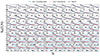 |
Fig. A.1. Separation energy Sn as a function of N for 80 isotopic chains with 21 ≤ Z ≤ 100. In blue, Sn maximizing and minimizing the uncorrelated mass uncertainties (Case 1). In red, Sn computed by maximizing and minimizing the uncorrelated Sn uncertainties (Case 2). In black, the mean of the uncorrelated Sn uncertainties. |
All Figures
|
Fig. 1. Case 1: Representation in the (N,Z) plane of the uncorrelated masses uncertainties, σM(Z, N) (in MeV), obtained from 10931 runs with σM,exp < 0.8 MeV. See Goriely & Capote (2014) for more details. The nuclei outlined with open magenta squares are the experimentally known masses. The dashed magenta line is a contour of nuclei with σM below 0.55 MeV. The shell closures are displayed as plain lines. |
| In the text | |
|
Fig. 2. Same as Fig. 1 but for Case 2: Uncorrelated Sn uncertainties (in MeV) determined in Case 2 within the BFMC method. |
| In the text | |
|
Fig. 3. rms values of Sn and Qβ when randomly picked Npick times from Case 1 or Case 2. The rms deviation is calculated with respect to all experimentally known Sn or Qβ values (Wang et al. 2021). The random pickup was done 200 times to obtain an average rms value. |
| In the text | |
|
Fig. 4. Two-neutron separation energy, S2n, for the Z = 70 isotopic chain obtained with 200 combinations for Case 1 (blue lines) and 200 for Case 2 (red lines). A zoom on the N = 126 shell gap shows its potential disappearance in Case 1, a clear sign of overestimating the uncertainties in this case. One specific extreme combination of Case 1, shown by the thick blue line, highlights the possible shell disappearance. |
| In the text | |
|
Fig. 5. Heat map representing the parameter uncertainty of Sn(Z, N − 1) (relative to HFB-24 values) as a function of Sn(Z, N) uncertainties (relative to HFB-24 values) for each BFMC combination selected in Case 2 (10643 combinations). The subplots use the same axis and are separated by isotopic chains to show the correlation for each of them. Each frame is 500 per 500 bins and each bin is color-coded to the number of combinations in it. |
| In the text | |
|
Fig. 6. Schematic view of the anticorrelations imposed by Sn and Qβ on the choices of mass uncertainties. When maximizing Sn(Z,N), we imposed Mmin(Z,N). The consequences of this choice are depicted in red, where the mass of (Z,N − 1) will need to be minimum and the mass of (Z+1,N − 1) maximum, due to the anticorrelation with Qβ. |
| In the text | |
|
Fig. 7. Convergence of the averaged uncertainties, |
| In the text | |
|
Fig. 8. Impact of the nuclear mass uncertainties obtained in Cases 1 to 4 on the mass fractions of stable nuclei (and long-lived Th and U) of the material ejected from the binary 1.38–1.38 M⊙ NSM model as a function of the atomic mass, A. Solar r-abundances (Goriely 1999) are shown in gray as a reference and are scaled to the peak value of the A = 130 abundance in the Case 1 simulation. |
| In the text | |
|
Fig. 9. NSM abundance uncertainties (in log scale) given by the ratio of maximum to minimum mass fractions (Xmax/Xmin) resulting from Sn uncertainties, as obtained in Cases 1 to 4. |
| In the text | |
|
Fig. 10. Same as Fig. 8 but for the impact of model vs. parameter mass uncertainties. The six nuclear models used here are described in Sect. 2.1. The insert zoomed in the lower panel shows the A > 120 range where r-process nucleosynthesis is dominantly impacted by the parameter and model uncertainties. The blue-shaded range gives the HFB-24 associated parameter uncertainties. |
| In the text | |
|
Fig. 11. Abundance uncertainties (Xmax/Xmin) for Case 4 vs. model uncertainties (using WS4, D1M, FRDM12, BSkG3, D3G3M, and HFB-24 models). Here, the model uncertainties are represented as if they would be uncorrelated, a common misrepresentation of the correlated model uncertainties (Martinet et al. 2024). |
| In the text | |
|
Fig. 12. Neutron capture rate uncertainties obtained from TALYS computations using Case 4 mass uncertainties. The reactions are color-coded by their parameter uncertainties (the ratio between maximum and minimum rates). |
| In the text | |
|
Fig. 13. Abundance uncertainties for Case 4 with and without propagation of the mass uncertainties to Hauser-Feshbach computations of neutron capture rates. |
| In the text | |
|
Fig. A.1. Separation energy Sn as a function of N for 80 isotopic chains with 21 ≤ Z ≤ 100. In blue, Sn maximizing and minimizing the uncorrelated mass uncertainties (Case 1). In red, Sn computed by maximizing and minimizing the uncorrelated Sn uncertainties (Case 2). In black, the mean of the uncorrelated Sn uncertainties. |
| In the text | |
Current usage metrics show cumulative count of Article Views (full-text article views including HTML views, PDF and ePub downloads, according to the available data) and Abstracts Views on Vision4Press platform.
Data correspond to usage on the plateform after 2015. The current usage metrics is available 48-96 hours after online publication and is updated daily on week days.
Initial download of the metrics may take a while.