| Issue |
A&A
Volume 691, November 2024
|
|
|---|---|---|
| Article Number | A125 | |
| Number of page(s) | 8 | |
| Section | Extragalactic astronomy | |
| DOI | https://doi.org/10.1051/0004-6361/202451732 | |
| Published online | 01 November 2024 | |
Photometric properties of classical bulge and pseudo-bulge galaxies at 0.5 ≤ z < 1.0
1
National Astronomical Observatories, Chinese Academy of Sciences, Beijing 100101, China
2
School of Astronomy and Space Science, University of Chinese Academy of Sciences, Beijing 100049, China
3
Key Laboratory of Space Astronomy and Technology, National Astronomical Observatories, Chinese Academy of Sciences, Beijing 100101, China
4
Institute for Frontiers in Astronomy and Astrophysics, Beijing Normal University, Beijing 102206, China
⋆ Corresponding author; This email address is being protected from spambots. You need JavaScript enabled to view it.
; This email address is being protected from spambots. You need JavaScript enabled to view it.
Received:
31
July
2024
Accepted:
26
September
2024
Abstract
Context. We compare the photometric properties and specific star formation rate (sSFR) of classical- and pseudo-bulge galaxies with M∗ ≥ 109.5 M⊙ at 0.5 ≤ z < 1.0, selected from all five CANDELS fields. We also compare these properties of bulge galaxies at lower redshift selected from MaNGA survey in previous work.
Aims. This paper aims to study the properties of galaxies with classical and pseudo-bulges at intermediate redshift, to compare the differences between different bulge types, and to understand the evolution of bulges with redshift.
Methods. Galaxies are classified into classical bulge and pseudo-bulge samples according to the Sérsic index n of the bulge component based on results of two-component decomposition of galaxies, as well as the position of bulges on the Kormendy diagram. For the 105 classical bulge and 86 pseudo-bulge galaxies selected, we compare their size, luminosity, and sSFR of various components.
Results. At a given stellar mass, most classical bulge galaxies have smaller effective radii, larger B/T, brighter and relatively larger bulges, and less active star formation than pseudo-bulge galaxies. In addition, the two types of galaxies have larger differences in sSFR at large radii than at the central region at both low- and mid-redshifts.
Conclusions. The differences between the properties of the two types of bulge galaxies are generally smaller at mid-redshift than at low-redshift, indicating that they are evolving to more distinct populations towards the local universe. Bulge type is correlated with the properties of their outer disks, and the correlation is already present at redshifts as high as 0.5 < z < 1.
Key words: galaxies: bulges / galaxies: evolution / galaxies: formation
© The Authors 2024
 Open Access article, published by EDP Sciences, under the terms of the Creative Commons Attribution License (https://creativecommons.org/licenses/by/4.0), which permits unrestricted use, distribution, and reproduction in any medium, provided the original work is properly cited.
This article is published in open access under the Subscribe to Open model. This email address is being protected from spambots. You need JavaScript enabled to view it. to support open access publication.
1. Introduction
In the central region of a spiral galaxy, there is often a bulge component that contains a higher concentration of stars and light compared to the disk component that extends to a larger radius (Sandage 1961). Bulges are classified into two main categories based on their properties observed at low-redshift. Like elliptical galaxies, typical classical bulges are dominated by random motion and follow the fundamental plane (Fisher & Drory 2016). In contrast, pseudo-bulges exhibit characteristics similar to disk galaxies, with rotational motion and notable substructures such as nuclear bars, spiral arms, and inner rings (Carollo et al. 1997; Erwin & Sparke 2002; Knapen 2005; Fisher & Drory 2011). In general, classical bulge galaxies are more massive, redder, with less star formation (Drory & Fisher 2007; Fisher et al. 2009; Fisher & Drory 2010; Wang et al. 2019; Sachdeva et al. 2020; Hashemizadeh et al. 2022; Kumar & Kataria 2022), and have larger central velocity dispersion (Kormendy et al. 2010; Fabricius et al. 2012; Sachdeva et al. 2020; Wang et al. 2024) than pseudo-bulge galaxies. At low-redshifts, bulge galaxies are observed from Local Group to redshift of 0.1 (Fisher et al. 2009; Fisher & Drory 2010; Kormendy et al. 2010; Kumar & Kataria 2022), and are found to increase their bulge-to-total ratio (B/T) through internal star formation (Fisher et al. 2009), to have an increasing or decreasing fraction of classical and pseudo-bulges towards higher redshift, and to be less axisymmetric for pseudo-bulges towards higher redshift (Kumar & Kataria 2022).
Theoretically, classical bulges are commonly attributed to violent processes such as clumpy collapse (Noguchi 1999; Elmegreen et al. 2008; Inoue & Saitoh 2012) and galaxy mergers (Aguerri et al. 2001; Hammer et al. 2005), while pseudo-bulges are thought to form slowly through secular evolution (Courteau et al. 1996; Kormendy & Kennicutt 2004; Athanassoula 2005; Fisher et al. 2009; Fisher & Drory 2010; Kormendy et al. 2010), involving mild gas inflow and stellar migration triggered by bars or spiral arms (Scannapieco et al. 2010; Bird et al. 2012; Guedes et al. 2013; Grand et al. 2014; Halle et al. 2015; Combes et al. 2020; Gargiulo et al. 2022). However, simulations, semi-empirical models (Hopkins et al. 2010; Guedes et al. 2013; Querejeta et al. 2015; Sauvaget et al. 2018; Fragkoudi et al. 2016; Kumar et al. 2021), and observations (Genzel et al. 2008; Eliche-Moral et al. 2013; Laurikainen & Salo 2016) indicate that bulge formation and evolution is more complicated than the general picture.
In the previous work of Hu et al. (2024), with the help of the MaNGA survey (Mapping Nearby Galaxies at Apache Point Observatory survey, Bundy et al. 2015) and two-component decomposition catalogue (Domínguez Sánchez et al. 2022), we compared the resolved properties of classical and pseudo-bulges and their host galaxies at 0.01 < z < 0.15. We found that at a given stellar mass, disks of pseudo-bulge galaxies are younger, have more active star formation, rotate more, and may contain more HI content compared with the disks of classical bulge galaxies. More interestingly, the differences between the properties of disks for the two types of bulge galaxies are larger than the differences between bulges themselves, indicating that the formation of bulges may be closely related to the evolution of outer disks in galaxies.
While most statistical studies of bulge properties focus on the low-redshift range, studying the bulge component of faraway galaxies is more difficult due to the limited resolution of observation. The central region of higher-redshift galaxies can be resolved only by space telescopes, such as Hubble Space Telescope (HST, Polidan 1991), James Webb Space Telescope (JWST, Gardner et al. 2006) and China Space Station Telescope (CSST, Zhan 2018). For example, Sachdeva et al. (2017) explored the growth of different types of bulge galaxies since z ∼ 1 using HST and find that classical bulges are brighter than pseudo ones at all redshift ranges. However, there are few studies about the other properties of bulges at mid-redshift.
In this work, to better investigate the properties of bulges and bulge galaxies at intermediate redshift, we studied galaxies of different types of bulges at 0.5 ≤ z < 1.0 from five CANDELS (Cosmic Assembly Near-infrared Deep Extragalactic Legacy Survey, Grogin et al. 2011; Koekemoer et al. 2011; Faber 2011) fields observed by HST. To select galaxies with bulge components, we performed two-component decomposition for the galaxies with M∗ ≥ 109.5 M⊙. Following the previous work of Hu et al. (2024), we divided selected samples into classical and pseudo-bulge galaxies using the criteria of bulge Sérsic index combined with the position of the bulges on the Kormendy diagram (Gadotti 2009). We compared the photometric properties of the bulges and disks including size and luminosity, as well as sSFR calculated by rest-frame UVI colour, and sSFR profiles for the two types of bulge galaxies.
This paper is organised as follows. Section 2 introduces how we selected galaxies with different types of bulges from CANDELS. Section 3 studies and compares the photometric properties of bulges and disks. Section 4 compares the specific star formation rate (sSFR) for the two types of bulges, their galaxies, and the sSFR profile of the galaxies. Our conclusions and discussion are presented in Section 5. Throughout the paper, we adopt a flat Λ-CDM concordance model (H0 = 70.0 km s−1 Mpc−1 and ΩM = 0.30).
2. Two-component decomposition and sample selection
We performed two-component decomposition fitting for 2178 galaxies with good image quality selected from five CANDLES fields; of these, we selected the 344 most reliable two-component galaxies. We then classified galaxies with classical and pseudo-bulges using criteria of both the bulge Sérsic index and the position of bulges on the Kormendy diagram. In the end, 105 classical bulge galaxies and 86 pseudo-bulge galaxies were selected.
2.1. Selection of two-component galaxies
For all sources in the five catalogues of CANDELS fields, including COSMOS (Cosmic Evolution Survey, Nayyeri et al. 2017), EGS (Extended Groth Strip, Stefanon et al. 2017), GOODS-N (Great Observatories Origins Deep Survey north, Barro et al. 2019), GOODS-S (Great Observatories Origins Deep Survey south, Guo et al. 2013), and UDS (UKIDSS Ultra-Deep Survey, Galametz et al. 2013), we first selected 2178 galaxies with image quality good enough for further decomposition fitting, following the criteria presented in the previous works of Liu et al. (2018) and Cui et al. (2024). The details of the selection criteria are listed below, and Table 1 presents the numbers of galaxies selected after applying each of the criteria.
Selection criteria and sample sizes for galaxies/sources in CANDELS.
– CLASS_STAR < 0.9 are sources identified as galaxies rather than stars, where CLASS_STAR is an output index from Source Extractor (SEXTRACTOR, Bertin & Arnouts 1996).
– Only galaxies with F160W(H) band magnitude (MH) brighter than 24.5 were selected, as these have signal-to-noise ratios high enough to get reliable images.
– GALFIT FLAG (H) = 0 selected galaxies that can be reliably fitted by GALFIT for F160W band images (van der Wel et al. 2012).
– Galaxies with redshifts in the range of 0.5 ≤ z < 1.0 were selected (see more detailed redshift measurements in Cui et al. (2024)).
– Small galaxies with  were removed. The stellar mass was calculated by fitting SPS models to broadband photometry using the code FAST (Kriek et al. 2009), based on models of Bruzual & Charlot (2003) with initial mass function of Chabrier (2003), exponentially declining τ-models of star formation history, solar metallicity, and a dust law of Calzetti et al. (2000).
– The criterion of the semi-major axis of whole galaxies (RSMA ≥ 0.18″, van der Wel et al. 2012) removed sources smaller than the full width half maximum (FWHM) of the point spread function (PSF) of the HST images (average value in F160W band of 0.18″).
– In the CANDELS catalogue, we selected galaxies that were marked by SExtractor with PhotFlag = 0, indicating that they are not contaminated by foreground sources or neighbouring objects, have no bad pixels, and are not located on the borders of the mosaic in the F160W band.
– We also visually inspected the images to ensure that the galaxies are uncontaminated in all bands of F160W, F606W, F814W, and F125W.
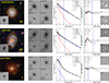 |
Fig. 1. Two-component decomposition results of three example galaxies with different types. Top to bottom: A classical bulge galaxy (cBG), a pseudo-bulge galaxy (pBG), and an elliptical galaxy (E) are shown in each row. Their IDs and types are shown in the top left and bottom right corners in the most left panels. In each row, from left to right: (1) The first panel shows the colour image and F160W image (inserted). The red and blue ellipses are the effective radii range of the bulge and disk components of the SerExp fitting. (2) The second panel displays the images from the Ser (top left subpanel) and SerExp (top right subpanel) models, where the SerExp model image is the sum of the model image of its bulge (bottom left subpanel) and disk (bottom right subpanel). The effect of the PSF has been included in these model images. The outputs of fitting for each model are shown on the left bottom corners of each subpanel, including Sérsic index (n), apparent magnitude (mag), effective radius (R), axial ratio (Ar), and position angle (Pa). (3) The third panel presents light profiles, where black dots are raw data, and the solid grey line displays the Ser model fitting result. The solid black line is SerExp model fitting result, which is the sum of its bulge and disk represented by the solid red and blue lines, where the PSF is also included. The vertical grey, red, and blue dash-dot lines are the effective radii of Ser model Re, bulge Rb, and disk Rd. (4) The fourth panel shows the 1D and 2D residuals. The grey square and black pentagon are the 1D residuals for the Ser and SerExp models respectively. The 2D residuals for Ser and SerExp are displayed on top and bottom right corners. |
Combining the above criteria, we ultimately selected 2178 galaxies to perform the two-component decomposition fitting using GALFIT. Firstly, we conducted pre-processing on the images of the sources before the fitting. We generated multi-band thumbnail images with a size of 401 × 401 pixels from the original CANDELS mosaics for individual targets. The sky background was subtracted using a pixel-by-pixel background estimation method. In addition, we took photometric parameters provided by SEXTRACTOR as the initial structural parameter priors for GALFIT (Peng et al. 2002).
Using GALFIT, we fitted F160W images of our selected galaxies using two photometric function models: a single Sérsic profile (Ser, Sérsic 1963), and a two-component model consisting of a Sérsic profile for the bulge and an exponential profile for the disk (SerExp). During the fitting process, we set some limitations. For both models, the range of index n on Sérsic profile was from 0.5 to 8 and the effective radius range was from 0.5 to 50 pixels. For SerExp models, we set the effective radii of disks to be larger than those of bulges (Rb < Rd), to ensure domination of disk components in the outer area. This provided us with the parameters of each galactic component for each photometric function model, such as effective radius, magnitude, axis ratio, and position angle.
Based on the fitting results of GALFIT, we selected the most robust two-component galaxy samples for which the SerExp model was preferred. In Fig. 1, we show examples of three galaxies that are identified as classical bulge + disk, pseudo-bulge + disk, and one-component elliptical by our method. The robust two-component galaxies were required to strictly adhere to all of the selection criteria below:
– According to both the F160W image and the colour image (obtained by combining the F606W, F814W, and F160W images), 778 galaxies were selected in which a brighter and more concentrated central component could be visually identified, together with an extended bluer component in the outer region with some structure, such as spiral arms or star formation clumps. For example, as shown in the leftmost three panels of Fig. 1, the top two galaxies exhibit brighter central components and bluer disks with spiral arms, while the bottom one shows a single smooth component.
– For a two-component galaxy, its bulge light is required to dominate in the inner region and its disk to dominate in the outer region by analysing the light profiles of different model fitting results. The one-dimensional residuals, representing the difference between real data and model data, must be smaller than ±0.1 at all radii. For example, in the third panel of the third column of Fig. 1, the light profile shows that its disk does not dominate in the outer region; thus, it is classified as a single-component galaxy. Based on these criteria, we selected 657 galaxies for which the SerExp model was preferred.
– The two-dimensional SerExp model images of the bulge and disk components reproduced well the bulges and disks in the F160W images, showing similar effective radius, axis ratio, and position angle visually between them. This also meant that the relative residuals from the two-dimensional SerExp modal data had to be closer to 0 at all pixels. For example, in the second and fourth columns of the first and second row in Fig. 1, the SerExp model results give good fitting to the images, with much smaller two-dimensional residuals. Therefore, 187 galaxies with inadequate results of the SerExp model were discarded.
– Robust bulge components were required to have effective radii greater than the HWHM of the PSF of the HST images (Gadotti 2009), which had an average value in F160W band of 0.09″. Thus, 126 galaxies with small bulges were removed.
Ultimately, 344 bulge+disk galaxies with reliable fitting results were selected to be analysed in this work. In addition, we also selected elliptical galaxies to set the Kormendy relation criterion for identifying bulge types in the following subsection. Similar to the example shown in the third row of Fig. 1, 392 elliptical candidates best-fitted by only one smooth component on F160W were selected. Combined with the large Sérsic index (3 < n < 7.95), 253 typical elliptical galaxies were selected.
We chose the F160W band to be studied and presented in this paper, because the images have higher signal-to-noise ratio than the other bands. Moreover, the F160W band is relatively close to the r-band in SDSS at rest-frame, which is generally considered the good band where bulge features are most prominent observationally (Fisher & Drory 2016). We also performed the same fitting procedures on images in other bands and checked that the obtained classification results of galaxy types remain similar.
2.2. Selection of classical and pseudo-bulge galaxies
To classify the bulge types in low-redshift galaxies, two common photometric criteria were used (Kormendy & Kennicutt 2004; Fisher & Drory 2016; Wang et al. 2019; Sachdeva et al. 2020). The first is the Sérsic index of the bulge component nb, because most classical bulges were found to have nb > 2 and most pseudo-bulges to have nb < 2 (e.g. Kormendy & Kennicutt 2004; Fisher & Drory 2016). The other criterion is the positions of the bulges on the Kormendy diagram (Kormendy 1977), where classical bulges are found to follow the Kormendy relation between effective radius Re and average surface brightness within the effective radius ⟨μe⟩ of elliptical galaxies, while pseudo-bulges normally deviate (Gadotti 2009). For mid-redshift galaxies, only a few studies have been done (Sachdeva et al. 2017; Sachdeva & Saha 2018). We visually inspected the central parts of these galaxies and found that bulges with structures such as inner ring, nuclear bar, and inner spiral mostly also have small nb and are located deviating from the Kormendy relation. Therefore, we selected our mid-redshift classical and pseudo-bulge samples, also using the criteria of nb = 2 combined with the Kormendy relation.
For the 344 two-component galaxies selected as described in the previous subsection, following the classification method of Hu et al. (2024), we first used nb = 2 as the divider to classify bulge types, thus obtaining 181 classical and 155 pseudo-bulge galaxies for our sample. In our previous works (Wang et al. 2019; Hu et al. 2024), we selected classical bulge galaxies with 3 < nb < 7.95 at low-redshift, to minimise the effect of uncertainty in fitting the bulge Sérsic index. In this work, in order to have a larger sample, we used 2 < nb < 7.95 to select classical bulge samples. We have checked that all conclusions in this paper remain unchanged when selecting classical bulges using 3 < nb < 7.95 instead.
For the criterion of positions on the Kormendy diagram, we first fitted the Kormendy relation of elliptical galaxies based on the 253 ellipticals selected as described in Section 2.1. Panel (a) of Fig. 2 shows the result:
 (1)
(1)
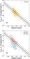 |
Fig. 2. The Kormendy relation. Panel (a): The Kormendy relation of our selected elliptical galaxies (E) in F160W band. The orange dots represent individual elliptical galaxies, and the black solid line is the best linear fitting of these dots. The two black dotted lines show the ±1σ scatter (σ = 0.74). Panel (b): On the Kormendy diagram, the positions of classical bulges (cB: red dots) and pseudo-bulges (pB: blue dots) constrained by both nb and Kormendy relation are plotted. |
We required the pseudo-bulges to lie below the lower dotted line in panel (a) of Fig. 2 and the classical bulges to lie above the lower dotted line. Combined with the criterion of the Sérsic index, we obtained 86 pseudo-bulges and 105 classical bulges. Their positions on the Kormendy diagram are indicated by blue and red dots in panel (b) of Fig. 2.
In Fig. 3, we compare the stellar mass and redshift of the selected galaxies with different types of bulges. In panel (a), the filled bars show the stellar mass distribution for classical and pseudo-bulge galaxies, and their peak values are 1010.7 M⊙ and 109.7 M⊙ respectively. For comparison, the unfilled bars are over-plotted, showing the results of galaxies at low-redshift from our previous work (panel (a) of Figure 2; Hu et al. 2024). The peak stellar masses are 1011.3 M⊙ and 109.9 M⊙ for classical and pseudo-bulge galaxies. The comparisons indicate that both types of bulge galaxies at low-redshift are more massive than galaxies at mid-redshift, and classical bulge galaxies are more massive than pseudo-bulge galaxies at all redshifts investigated. Panels (b) and (c) of Fig. 3 show that redshifts of two types of bulges both have wide distributions, independent of stellar mass.
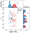 |
Fig. 3. Distributions of galaxy total stellar mass and redshift for our selected classical bulge galaxies (cBG: red symbols) and pseudo-bulge galaxies (pBG: blue symbols). Panel (b) presents redshift as a function of galaxy total stellar mass. Each dot indicates an individual galaxy. The solid lines show median relations and dashed lines enclose 68% scatter. Panels (a) and (c) present the distributions of the two properties respectively. In panel (a), unfilled histograms are over-plotted, showing distributions of samples at low-redshift from the previous work of Hu et al. (2024). |
3. Photometric properties of bulges and bulge galaxies
In this section, we compare the size and absolute magnitude of the selected classical and pseudo-bulges, and those of their host galaxies, as a function of galaxy stellar mass. The results are also compared with the properties of bulges and bulge galaxies studied in our previous work at low-redshift (Hu et al. 2024), offering clues as to the evolution of bulges with cosmic time.
Note that bulge samples selected in this work from CANDELS and those selected at low-redshift by Hu et al. (2024) were obtained using two-component fitting in bands with different wavelengths. F160W band is used for mid-redshift samples from the CANDELS survey, and the corresponding rest-frame wavelength was 8000 Å for galaxies at z = 1. For the low-redshift MaNGA sample, we used the SDSS r-band (6165 Å) for analyses. Caution must be exercised when interpreting the comparison between the two.
3.1. Size of bulges and bulge galaxies
In Fig. 4, we compare the sizes of bulges of different types and the sizes of their host galaxies and disk components. The effective radius of each component has been adopted to represent the size, which is from the two-component decomposition fitting as described in Section 2.1.
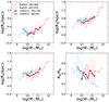 |
Fig. 4. Sizes of bulges and bulge galaxies. Effective radii of bulges (Rb, top left panel), disks (Rd, top right panel), and whole galaxies (Re, bottom left panel) as a function of galaxy stellar mass. Ratios of bulge effective radius to the effective radius of the whole galaxy (Rb/Re, bottom right panel) as a function of galaxy stellar mass. The median values are indicated by red triangles for classical bulge samples and blue circles for pseudo-bulge samples. The error bars show the 1σ scatter. Dark colour represents results of the selected samples from CANDELS in this work, and light colour represents results of the samples selected at low-redshift from MaNGA by Hu et al. (2024). |
The top left panel of Fig. 4 compares the sizes of bulges. For CANDELS galaxies, the sizes of pseudo-bulges decrease at M∗ < 1010 M⊙ and become almost flat or with a slight increase at larger masses. For classical bulges, their sizes remain similar at M∗ < 1010.6 M⊙ and then increase with stellar mass. Both types of bulges have similar sizes in the overlapped region of stellar mass. Compared with the low-redshift bulge samples selected by Hu et al. (2024), as indicated by light symbols and lines, the sizes of both types of bulges are similar at different redshifts, except in the case of pseudo-bulges in galaxies less massive than ∼ 109.8 M⊙.
In the top right of Fig. 4, for both classical and pseudo-bulge galaxies, the disk effective radius (Rd) increases with stellar mass for M∗ > 1010 M⊙. Disks of pseudo-bulge galaxies are a bit larger than disks of classical ones with similar stellar mass. This general trend is consistent with low-redshift samples, with a larger difference between bulge types at low-redshift than at mid-redshift. Compared with the top left panel of Fig. 4, larger differences exist in disk size than in bulge size between classical and pseudo-bulge galaxies, at both low and mid-redshifts. For the effective radius of the whole galaxies as shown in the bottom left of Fig. 4, a similar trend is seen in the radius of disks. The difference between galaxies with different bulge types is even larger, mainly due to a larger B/T of classical bulge galaxies, as will be seen in Fig. 5.
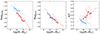 |
Fig. 5. Absolute magnitude of bugle components (left panel), disk components (middle panel), and luminosity B/T (right panel) as a function of stellar mass. The symbols and lines represent the same samples as in Fig. 4. |
We checked the relative size of bulges to the whole galaxies in the bottom right panel of Fig. 4. For pseudo-bulge galaxies, the relative bulge size decreases significantly with stellar mass. For classical ones, the dependence on stellar mass is much smaller. In the overlapped mass range of 1010.2−10.4 M⊙, pseudo-bulge galaxies have relatively smaller bulges than classical ones. The difference between the two bulge type galaxies is much larger for low-redshift samples than for mid-redshift samples, mainly due to the smaller sizes of classical bulge galaxies at low-redshift.
3.2. Absolute magnitude and B/T
We compare in Fig. 5 the absolute magnitude of our selected classical and pseudo-bulges, the absolute magnitude of disks of their host galaxies, and the luminosity B/T of their host galaxies. The absolute magnitude of bulges and disks are from the results of two-component decomposition as described in Section 2.1. B/T is the ratio between bulge luminosity and total luminosity of both bulge and disk components.
The left panel of Fig. 5 shows that for galaxies both at mid- and low-redshifts, bulges are brighter in more massive galaxies. In addition, classical bulges are brighter than pseudo-bulges in galaxies at given stellar mass at both mid- and low-redshifts. The result is consistent with Sachdeva et al. (2017), which shows that classical bulges are brighter than pseudo-bulges in B-band and I-band at 0.4 ≤ z < 1.0 and 0.02 ≤ z < 0.05.
In the middle panel of Fig. 5, with stellar mass increasing, the absolute magnitude of disks is brighter, at both mid- and low-redshifts. The absolute magnitude of the disks in the two types of galaxies is more similar at mid-redshift than at low-redshift, with obviously brighter disks in pseudo-bulge galaxies than in classical bulge galaxies at low-redshift. The results are also consistent with those studied in Sachdeva et al. (2017) in B- and I-band.
In the right panel of Fig. 5, we compare the B/T for classical and pseudo-bulge galaxies as a function of galaxy stellar mass. At mid-redshift, pseudo-bulge galaxies have obviously smaller bulge fractions than classical ones at given stellar mass. Similar results have been derived by Sachdeva & Saha (2018) when comparing the B/T of classical and pseudo-bulge galaxies in B-band at 0.4 < z < 1.0. At low-redshift, the difference in B/T between classical and pseudo-bulge galaxies is even larger. In particular, for classical bulge galaxies at stellar mass less than 1010.8 M⊙, B/T increases with stellar mass at mid-redshift while decreases with stellar mass at low-redshift. The large B/T of classical bulge galaxies leads to smaller effective radii of the galaxies, and makes the difference in Re more prominent than the difference in Rd between pseudo-bulge and classical bulge galaxies, as seen in Fig. 4.
4. The sSFR of bulges and bulge galaxies
In this section, we study and compare spatially resolved sSFR for the selected galaxies with classical and pseudo-bulges. For galaxies at mid-redshift from CANDELS, the sSFR of each pixel in a given galaxy is estimated based on the position of galaxies on the rest-frame UVI colour diagram, as shown in the top right panel of Fig. 10 in Cui et al. (2024) and Wang et al. (2017). This new method is used to determine the sSFR values, which have been tested to be consistent with results from broadband stellar population fitting from UV to Infrared (Fang et al. 2018). Details regarding estimating rest-frame UVI colour and sSFR can be found in Appendices A and B of Cui et al. (2024).
For comparison, we also show the sSFR for bulge galaxies at low-redshift in MaNGA selected by Hu et al. (2024). Star formation rate (SFR) on each pixel of these galaxies is calculated according to Hα flux by empirical law of Kennicutt (1998, equation 2), where flux of Hα and stellar mass on each pixel of these MaNGA galaxies are from full spectrum fitting (Cappellari & Emsellem 2004; Cappellari 2017; Ge et al. 2018, 2019, 2021). As we will see in Fig. 6 and Fig. 7, there is a systematic difference, up to two orders of magnitude, in the sSFR derived from the different methods applied to low- and mid-redshift galaxies. About one order of magnitude difference in sSFR at given stellar mass can be due to the intrinsic difference between galaxies at a higher redshift of z = 1 and galaxies at z = 0, as studied by Moster et al. (2018) and Behroozi et al. (2019). Moster et al. (2018) compared sSFR of the same galaxies estimated from different methods, and find that the difference in sSFR values from Hα and rest-frame UVI diagram is small. Therefore, the other one order of magnitude difference in sSFR between galaxies at low- and mid-redshifts may be caused by different IMFs, flux calibrations, and other possible effects of spectral processing techniques.
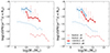 |
Fig. 6. For galaxies with classical bulges and pseudo-bulges, sSFR within Re (left panel) and Rb (right panel) as a function of galaxy stellar mass. The symbols and colours represent the same samples as in Fig. 4. |
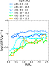 |
Fig. 7. Specific star formation rate radial profiles of selected classical (triangles) and pseudo-bulge galaxies (circles). Results are shown in galaxy stellar mass intervals of 0.5 in logarithmic space as indicated on the top of the panel using different colours. |
In the left panel of Fig. 6, we compare the average sSFR within Re of classical and pseudo-bulge galaxies indicated by red and blue symbols and lines. This value can be considered to represent the strength of star formation activities of the whole galaxies, since the average values of sSFR within an ellipse with a given radius vary with increasing radii R and gradually become stable at R ≥ Re. For galaxies at both redshifts, we find that galaxies with pseudo-bulges have more active star formation than galaxies with classical bulges at a given stellar mass. In addition, the difference in sSFR between classical and pseudo-bulge galaxies at mid-redshift is much smaller than that of galaxies at low-redshift.
For the bulge components, we compared the sSFR within Rb to reflect the bulge star formation activities, and the results are shown in the right panel of Fig. 6. The sSFR of classical bulges is a bit smaller than that of pseudo-bulges at a given stellar mass at both mid- and low-redshifts. However, the difference between bulge types at mid-redshift is obviously smaller than that at low-redshift, and is also smaller than the difference between galaxies that host different types of bulges as shown in the left panel. This may indicate an evolution trend of different types of bulges to somehow deviate more in star formation activities from z = 1 to z = 0.
In Fig. 7, we further check the profiles of the sSFR of galaxies with classical and pseudo-bulge at mid-redshift, to investigate in more detail the star formation activities in different components of galaxies. The median sSFR for each galaxy sample is shown as a function of radius. The influence of PSF on the spectrum was considered, and the innermost points of galaxies were chosen to be greater than their HWHM. Looking at the blue symbols in Fig. 7, for galaxies with stellar mass in the range 109.5−10 M⊙, the sSFR profiles are generally flat, with slightly increasing for both types of bulge galaxies. For galaxies more massive than 1010 M⊙, the sSFR profiles increase with increasing radius. Comparing the two types of bulge galaxies within the same stellar mass range, the sSFR of pseudo-bulge galaxies is similar and becomes larger than the classical ones from the centre to the outer regions.
Comparing the sSFR profiles of galaxies at mid-redshift as shown in Fig. 7 with the results of low-redshift galaxies as shown in the middle panel of Fig. 10 from Hu et al. (2024), the difference between the two bulge type galaxies is smaller at mid-redshift than at low-redshift, consistent with the trend seen in Fig. 6. Moreover, the slopes of sSFR for galaxies at mid-reshift are basically monotonic, while at low-redshift pseudo-bulge galaxies mostly have peak sSFR at radius of around 0.8 − 1.4Re. The evolution of sSFR slopes of pseudo-bulge galaxies may offer a hint as to the co-evolution of the bulge and the disk components.
5. Summary
In this paper, we compare photometric properties and sSFR of classical and pseudo-bulges and their host galaxies at 0.5 ≤ z < 1.0 selected from the CANDELS survey. We also compare the results with those derived at low-redshift, based on the samples selected from MaNGA survey in an earlier work of Hu et al. (2024). The galaxies with classical bulge and pseudo-bulge are selected based on the Sérsic index n of bulge component by two-component decomposition fitting, combined with the criterion of the position of bulges on the Kormendy diagram.
At both mid- and low-redshifts, classical bulge galaxies are more massive than pseudo-bulge galaxies. At a given stellar mass, most classical bulge galaxies have smaller effective radii of all components, larger B/T, brighter and relatively larger bulges, and lower sSFR at all radii than pseudo-bulge galaxies. However, the differences in most properties between the two types of bulge galaxies are in general smaller at mid-redshift than at low-redshift, indicating that these two types of bulges and their galaxies are evolving to more distinct populations towards the local universe.
In addition, the difference in central sSFR between classical and pseudo-bulge galaxies is smaller than the difference at larger radii for mid-redshift galaxies, which is consistent with what was previously discovered in Hu et al. (2024). Therefore, the co-evolution of bulges with their host galaxies and outer disks is already present at redshifts as high as 0.5 ≤ z < 1.
While it is difficult to simulate the formation and evolution of galactic bulges precisely due to the numerical effect suffered (Zeng et al. 2024), in future works, we will further study the observational properties of bulge galaxies at higher redshift, based on analysis of two-component decomposition fitting for galaxies at 1.0 ≤ z < 3.0 selected from JWST within five CANDELS fields.
Acknowledgments
This work is supported by the National Natural Science Foundation of China (grant No. 11988101), the National SKA Program of China (Nos. 2022SKA0110200, 2022SKA0110201), the National Key Research and Development Program of China (No. 2023YFB3002500), the Strategic Priority Research Program of Chinese Academy of Sciences, (grant No. XDB0500203), and K.C. Wong Education Foundation. JG acknowledges support from the Beijing Municipal Natural Science Foundation (No. 1242032), the Youth Innovation Promotion Association of the Chinese Academy of Sciences (No. 2022056), and the science research grants from the China Manned Space Project.
References
- Aguerri, J. A. L., Balcells, M., & Peletier, R. F. 2001, A&A, 367, 428 [NASA ADS] [CrossRef] [EDP Sciences] [Google Scholar]
- Athanassoula, E. 2005, MNRAS, 358, 1477 [NASA ADS] [CrossRef] [Google Scholar]
- Barro, G., Pérez-González, P. G., Cava, A., et al. 2019, ApJS, 243, 22 [NASA ADS] [CrossRef] [Google Scholar]
- Behroozi, P., Wechsler, R. H., Hearin, A. P., & Conroy, C. 2019, MNRAS, 488, 3143 [NASA ADS] [CrossRef] [Google Scholar]
- Bertin, E., & Arnouts, S. 1996, A&AS, 117, 393 [NASA ADS] [CrossRef] [EDP Sciences] [Google Scholar]
- Bird, J. C., Kazantzidis, S., & Weinberg, D. H. 2012, MNRAS, 420, 913 [NASA ADS] [CrossRef] [Google Scholar]
- Bruzual, G., & Charlot, S. 2003, MNRAS, 344, 1000 [NASA ADS] [CrossRef] [Google Scholar]
- Bundy, K., Bershady, M. A., Law, D. R., et al. 2015, ApJ, 798, 7 [Google Scholar]
- Calzetti, D., Armus, L., Bohlin, R. C., et al. 2000, ApJ, 533, 682 [NASA ADS] [CrossRef] [Google Scholar]
- Cappellari, M. 2017, MNRAS, 466, 798 [Google Scholar]
- Cappellari, M., & Emsellem, E. 2004, PASP, 116, 138 [Google Scholar]
- Carollo, C. M., Stiavelli, M., de Zeeuw, P. T., & Mack, J. 1997, AJ, 114, 2366 [NASA ADS] [CrossRef] [Google Scholar]
- Chabrier, G. 2003, PASP, 115, 763 [Google Scholar]
- Combes, F. 2020, in Galactic Dynamics in the Era of Large Surveys, eds. M. Valluri, & J. A. Sellwood, 353, 155 [NASA ADS] [Google Scholar]
- Courteau, S., de Jong, R. S., & Broeils, A. H. 1996, ApJ, 457, L73 [NASA ADS] [Google Scholar]
- Cui, Q., Zhao, P., & Liu, F. S. 2024, ApJ, 973, 52 [NASA ADS] [CrossRef] [Google Scholar]
- Domínguez Sánchez, H., Margalef, B., Bernardi, M., & Huertas-Company, M. 2022, MNRAS, 509, 4024 [Google Scholar]
- Drory, N., & Fisher, D. B. 2007, ApJ, 664, 640 [NASA ADS] [CrossRef] [Google Scholar]
- Eliche-Moral, M. C., González-García, A. C., Aguerri, J. A. L., et al. 2013, A&A, 552, A67 [NASA ADS] [CrossRef] [EDP Sciences] [Google Scholar]
- Elmegreen, B. G., Bournaud, F., & Elmegreen, D. M. 2008, ApJ, 688, 67 [NASA ADS] [CrossRef] [Google Scholar]
- Erwin, P., & Sparke, L. S. 2002, AJ, 124, 65 [Google Scholar]
- Faber, S. 2011, The Cosmic Assembly Near-IR Deep Extragalactic Legacy Survey (CANDELS) [Google Scholar]
- Fabricius, M. H., Saglia, R. P., Fisher, D. B., et al. 2012, ApJ, 754, 67 [Google Scholar]
- Fang, J. J., Faber, S. M., Koo, D. C., et al. 2018, ApJ, 858, 100 [NASA ADS] [CrossRef] [Google Scholar]
- Fisher, D. B., & Drory, N. 2010, ApJ, 716, 942 [NASA ADS] [CrossRef] [Google Scholar]
- Fisher, D. B., & Drory, N. 2011, ApJ, 733, L47 [NASA ADS] [CrossRef] [Google Scholar]
- Fisher, D. B., & Drory, N. 2016, Astrophys. Space Sci. Lib., 418, 41 [NASA ADS] [CrossRef] [Google Scholar]
- Fisher, D. B., Drory, N., & Fabricius, M. H. 2009, ApJ, 697, 630 [CrossRef] [Google Scholar]
- Fragkoudi, F., Athanassoula, E., & Bosma, A. 2016, MNRAS, 462, L41 [NASA ADS] [CrossRef] [Google Scholar]
- Gadotti, D. A. 2009, MNRAS, 393, 1531 [Google Scholar]
- Galametz, A., Grazian, A., Fontana, A., et al. 2013, ApJS, 206, 10 [Google Scholar]
- Gardner, J. P., Mather, J. C., Clampin, M., et al. 2006, Space Sci. Rev., 123, 485 [Google Scholar]
- Gargiulo, I. D., Monachesi, A., Gómez, F. A., et al. 2022, MNRAS, 512, 2537 [NASA ADS] [CrossRef] [Google Scholar]
- Ge, J., Yan, R., Cappellari, M., et al. 2018, MNRAS, 478, 2633 [NASA ADS] [CrossRef] [Google Scholar]
- Ge, J., Mao, S., Lu, Y., Cappellari, M., & Yan, R. 2019, MNRAS, 485, 1675 [NASA ADS] [CrossRef] [Google Scholar]
- Ge, J., Mao, S., Lu, Y., et al. 2021, MNRAS, 507, 2488 [NASA ADS] [CrossRef] [Google Scholar]
- Genzel, R., Burkert, A., Bouché, N., et al. 2008, ApJ, 687, 59 [Google Scholar]
- Grand, R. J. J., Kawata, D., & Cropper, M. 2014, MNRAS, 439, 623 [NASA ADS] [CrossRef] [Google Scholar]
- Grogin, N. A., Kocevski, D. D., Faber, S. M., et al. 2011, ApJS, 197, 35 [NASA ADS] [CrossRef] [Google Scholar]
- Guedes, J., Mayer, L., Carollo, M., & Madau, P. 2013, ApJ, 772, 36 [NASA ADS] [CrossRef] [Google Scholar]
- Guo, Y., Ferguson, H. C., Giavalisco, M., et al. 2013, ApJS, 207, 24 [NASA ADS] [CrossRef] [Google Scholar]
- Halle, A., Di Matteo, P., Haywood, M., & Combes, F. 2015, A&A, 578, A58 [NASA ADS] [CrossRef] [EDP Sciences] [Google Scholar]
- Hammer, F., Flores, H., Elbaz, D., et al. 2005, A&A, 430, 115 [NASA ADS] [CrossRef] [EDP Sciences] [Google Scholar]
- Hashemizadeh, A., Driver, S. P., Davies, L. J. M., et al. 2022, MNRAS, 515, 1175 [NASA ADS] [CrossRef] [Google Scholar]
- Hopkins, P. F., Bundy, K., Croton, D., et al. 2010, ApJ, 715, 202 [Google Scholar]
- Hu, J., Wang, L., Ge, J., Zhu, K., & Zeng, G. 2024, MNRAS, 529, 4565 [CrossRef] [Google Scholar]
- Inoue, S., & Saitoh, T. R. 2012, MNRAS, 422, 1902 [NASA ADS] [CrossRef] [Google Scholar]
- Kennicutt, R. C., Jr 1998, ARA&A, 36, 189 [NASA ADS] [CrossRef] [Google Scholar]
- Knapen, J. H. 2005, A&A, 429, 141 [NASA ADS] [CrossRef] [EDP Sciences] [Google Scholar]
- Koekemoer, A. M., Faber, S. M., Ferguson, H. C., et al. 2011, ApJS, 197, 36 [NASA ADS] [CrossRef] [Google Scholar]
- Kormendy, J. 1977, ApJ, 218, 333 [NASA ADS] [CrossRef] [Google Scholar]
- Kormendy, J., & Kennicutt, R. C., Jr 2004, ARA&A, 42, 603 [NASA ADS] [CrossRef] [Google Scholar]
- Kormendy, J., Drory, N., Bender, R., & Cornell, M. E. 2010, ApJ, 723, 54 [Google Scholar]
- Kriek, M., van Dokkum, P. G., Labbé, I., et al. 2009, ApJ, 700, 221 [Google Scholar]
- Kumar, A., & Kataria, S. K. 2022, MNRAS, 514, 2497 [CrossRef] [Google Scholar]
- Kumar, A., Das, M., & Kataria, S. K. 2021, MNRAS, 506, 98 [NASA ADS] [CrossRef] [Google Scholar]
- Laurikainen, E., & Salo, H. 2016, Astrophys Space Sci. Lib., 418, 77 [NASA ADS] [CrossRef] [Google Scholar]
- Liu, F. S., Jia, M., Yesuf, H. M., et al. 2018, ApJ, 860, 60 [NASA ADS] [CrossRef] [Google Scholar]
- Moster, B. P., Naab, T., & White, S. D. M. 2018, MNRAS, 477, 1822 [Google Scholar]
- Nayyeri, H., Hemmati, S., Mobasher, B., et al. 2017, ApJS, 228, 7 [NASA ADS] [CrossRef] [Google Scholar]
- Noguchi, M. 1999, ApJ, 514, 77 [NASA ADS] [CrossRef] [Google Scholar]
- Peng, C. Y., Ho, L. C., Impey, C. D., & Rix, H.-W. 2002, AJ, 124, 266 [Google Scholar]
- Polidan, R. 1991, 29th Aerospace Sciences Meeting, 402 [Google Scholar]
- Querejeta, M., Eliche-Moral, M. C., Tapia, T., et al. 2015, A&A, 579, L2 [NASA ADS] [CrossRef] [EDP Sciences] [Google Scholar]
- Sachdeva, S., & Saha, K. 2018, MNRAS, 478, 41 [NASA ADS] [CrossRef] [Google Scholar]
- Sachdeva, S., Saha, K., & Singh, H. P. 2017, ApJ, 840, 79 [NASA ADS] [CrossRef] [Google Scholar]
- Sachdeva, S., Ho, L. C., Li, Y. A., & Shankar, F. 2020, ApJ, 899, 89 [NASA ADS] [CrossRef] [Google Scholar]
- Sandage, A. 1961, The Hubble Atlas of Galaxies (Carnegie Institution of Washington Washington, DC) [Google Scholar]
- Sauvaget, T., Hammer, F., Puech, M., et al. 2018, MNRAS, 473, 2521 [NASA ADS] [CrossRef] [Google Scholar]
- Scannapieco, C., Gadotti, D. A., Jonsson, P., & White, S. D. M. 2010, MNRAS, 407, L41 [NASA ADS] [CrossRef] [Google Scholar]
- Sérsic, J. L. 1963, Boletin de la Asociacion Argentina de Astronomia La Plata Argentina, 6, 41 [Google Scholar]
- Stefanon, M., Yan, H., Mobasher, B., et al. 2017, ApJS, 229, 32 [NASA ADS] [CrossRef] [Google Scholar]
- van der Wel, A., Bell, E. F., Häussler, B., et al. 2012, ApJS, 203, 24 [NASA ADS] [CrossRef] [Google Scholar]
- Wang, W., Faber, S. M., Liu, F. S., et al. 2017, MNRAS, 469, 4063 [CrossRef] [Google Scholar]
- Wang, L., Wang, L., Li, C., et al. 2019, MNRAS, 484, 3865 [NASA ADS] [CrossRef] [Google Scholar]
- Wang, X., Luo, Y., Faber, S. M., et al. 2024, MNRAS, 533, 2026 [CrossRef] [Google Scholar]
- Zeng, G., Wang, L., Gao, L., & Yang, H. 2024, MNRAS, 532, 2558 [NASA ADS] [CrossRef] [Google Scholar]
- Zhan, H. 2018, 42nd COSPAR Scientific Assembly, 42, E1.16-4-18 [Google Scholar]
All Tables
All Figures
|
Fig. 1. Two-component decomposition results of three example galaxies with different types. Top to bottom: A classical bulge galaxy (cBG), a pseudo-bulge galaxy (pBG), and an elliptical galaxy (E) are shown in each row. Their IDs and types are shown in the top left and bottom right corners in the most left panels. In each row, from left to right: (1) The first panel shows the colour image and F160W image (inserted). The red and blue ellipses are the effective radii range of the bulge and disk components of the SerExp fitting. (2) The second panel displays the images from the Ser (top left subpanel) and SerExp (top right subpanel) models, where the SerExp model image is the sum of the model image of its bulge (bottom left subpanel) and disk (bottom right subpanel). The effect of the PSF has been included in these model images. The outputs of fitting for each model are shown on the left bottom corners of each subpanel, including Sérsic index (n), apparent magnitude (mag), effective radius (R), axial ratio (Ar), and position angle (Pa). (3) The third panel presents light profiles, where black dots are raw data, and the solid grey line displays the Ser model fitting result. The solid black line is SerExp model fitting result, which is the sum of its bulge and disk represented by the solid red and blue lines, where the PSF is also included. The vertical grey, red, and blue dash-dot lines are the effective radii of Ser model Re, bulge Rb, and disk Rd. (4) The fourth panel shows the 1D and 2D residuals. The grey square and black pentagon are the 1D residuals for the Ser and SerExp models respectively. The 2D residuals for Ser and SerExp are displayed on top and bottom right corners. |
| In the text | |
|
Fig. 2. The Kormendy relation. Panel (a): The Kormendy relation of our selected elliptical galaxies (E) in F160W band. The orange dots represent individual elliptical galaxies, and the black solid line is the best linear fitting of these dots. The two black dotted lines show the ±1σ scatter (σ = 0.74). Panel (b): On the Kormendy diagram, the positions of classical bulges (cB: red dots) and pseudo-bulges (pB: blue dots) constrained by both nb and Kormendy relation are plotted. |
| In the text | |
|
Fig. 3. Distributions of galaxy total stellar mass and redshift for our selected classical bulge galaxies (cBG: red symbols) and pseudo-bulge galaxies (pBG: blue symbols). Panel (b) presents redshift as a function of galaxy total stellar mass. Each dot indicates an individual galaxy. The solid lines show median relations and dashed lines enclose 68% scatter. Panels (a) and (c) present the distributions of the two properties respectively. In panel (a), unfilled histograms are over-plotted, showing distributions of samples at low-redshift from the previous work of Hu et al. (2024). |
| In the text | |
|
Fig. 4. Sizes of bulges and bulge galaxies. Effective radii of bulges (Rb, top left panel), disks (Rd, top right panel), and whole galaxies (Re, bottom left panel) as a function of galaxy stellar mass. Ratios of bulge effective radius to the effective radius of the whole galaxy (Rb/Re, bottom right panel) as a function of galaxy stellar mass. The median values are indicated by red triangles for classical bulge samples and blue circles for pseudo-bulge samples. The error bars show the 1σ scatter. Dark colour represents results of the selected samples from CANDELS in this work, and light colour represents results of the samples selected at low-redshift from MaNGA by Hu et al. (2024). |
| In the text | |
|
Fig. 5. Absolute magnitude of bugle components (left panel), disk components (middle panel), and luminosity B/T (right panel) as a function of stellar mass. The symbols and lines represent the same samples as in Fig. 4. |
| In the text | |
|
Fig. 6. For galaxies with classical bulges and pseudo-bulges, sSFR within Re (left panel) and Rb (right panel) as a function of galaxy stellar mass. The symbols and colours represent the same samples as in Fig. 4. |
| In the text | |
|
Fig. 7. Specific star formation rate radial profiles of selected classical (triangles) and pseudo-bulge galaxies (circles). Results are shown in galaxy stellar mass intervals of 0.5 in logarithmic space as indicated on the top of the panel using different colours. |
| In the text | |
Current usage metrics show cumulative count of Article Views (full-text article views including HTML views, PDF and ePub downloads, according to the available data) and Abstracts Views on Vision4Press platform.
Data correspond to usage on the plateform after 2015. The current usage metrics is available 48-96 hours after online publication and is updated daily on week days.
Initial download of the metrics may take a while.