| Issue |
A&A
Volume 691, November 2024
|
|
|---|---|---|
| Article Number | A31 | |
| Number of page(s) | 8 | |
| Section | Planets and planetary systems | |
| DOI | https://doi.org/10.1051/0004-6361/202451329 | |
| Published online | 25 October 2024 | |
Physical properties of trans-Neptunian object (143707) 2003 UY117 derived from stellar occultation and photometric observations
1
Instituto de Astrofísica de Andalucía, IAA-CSIC,
Glorieta de la Astronomía s/n,
18008
Granada,
Spain
2
Institut Polytechnique des Sciences Avancées IPSA,
94200
Ivrysur-Seine,
France
3
IMCCE, Observatoire de Paris, PSL Research University, CNRS, Sorbonne Université,
Univ. Lille,
75014
Paris,
France
4
Federal University of Technology-Paraná (UTFPR/PPGFA),
Curitiba,
PR,
Brazil
5
Laboratório Interinstitucional de e-Astronomia - LIneA - and INCT do e-Universo,
Av. Pastor Martin Luther King Jr, 126 - Del Castilho, Nova América Offices, Torre 3000 / sala 817,
Rio de Janeiro,
RJ
20765-000,
Brazil
6
LESIA, Observatoire de Paris, Université PSL, CNRS, Sorbonne Université,
5 place Jules Janssen,
92190
Meudon,
France
7
Florida Space Institute, University of Central Florida,
Orlando,
FL
32826-0650,
USA
8
Federal University of Uberlândia (UFU), Physics Institute,
Av. João Naves de Ávila 2121,
Uberlândia,
MG
38408-100,
Brazil
9
Universidade do Rio de Janeiro - Observatório do Valongo,
Ladeira do Pedro Antonio 43,
Rio de Janeiro,
RJ
20.080-090,
Brazil
10
Federal University of Technology - Paraná (PPGFA/UTFPR-Curitiba),
Av. Sete de Setembro,
3165
Curitiba,
PR,
Brazil
11
Departments of Astronomy and of Earth and Planetary Science,
501 Campbell Hall, University of California,
Berkeley,
CA
94720,
USA
12
naXys, Department of Mathematics, University of Namur,
Rue de Bruxelles 61,
5000
Namur,
Belgium
13
Observatório Nacional/MCTI,
Rua Gal. José Cristino 77,
Rio de Janeiro
RJ
20921-400,
Brazil
14
UNESP-São Paulo State University, Grupo de Dinâmica Orbital e Planetologia, CEP
12516-410
Guaratinguetá,
SP,
Brazil
15
Sociedad Astronómica Granadina,
Apartado de Correos 195,
18080
Granada,
Spain
16
Agrupación Astronómica de Eivissa,
C. Lucio Oculacio s/n,
07800
Ibiza,
Spain
17
Observatorio Astronómico de Albox,
Apt. 63, 04800 Albox,
Almeria,
Spain
18
Astronomical Institute of the Romanian Academy,
5 Cut¸itul de Argint,
040557
Bucharest,
Romania
19
Centro Astronómico Hispano en Andalucía, Observatorio de Calar Alto,
Sierra de los Filabres,
04550
Gérgal, Almeria,
Spain
20
University of Liège,
4000
Liège,
Belgium
21
Instituto de Astrofísica de Canarias (IAC),
C/Vía Láctea s/n,
38205
La Laguna,
Tenerife,
Spain
22
Instituto de Física Aplicada a las Ciencias y las Tecnologías, Universidad de Alicante,
Alicante,
San Vicente del Rapeig,
Spain
23
Agrupación Astronómica de Sabadell,
Prat de la Riba sn,
08206
Sabadell,
Spain
24
International Occultation Timing Association/European Section,
Am Brombeerhag 13,
30459
Hannover,
Germany
25
Rue de Mariembourg 45,
5670
Dourbes,
Belgium
26
TÜBITAK National Observatory,
Akdeniz University Campus,
07058
Antalya,
Turkey
27
Department of Astronomy and Space Sciences, Faculty of Science, Istanbul University,
34116
Istanbul,
Turkey
28
Istanbul University Observatory Research and Application Centre,
34116
Istanbul,
Turkey
29
School of Mathematical and Physical Sciences, Macquarie University,
Sydney
NSW
2109,
Australia
30
Astrophysics and Space Technologies Research Centre, Macquarie University,
Sydney
NSW
2109,
Australia
★ Corresponding author; This email address is being protected from spambots. You need JavaScript enabled to view it.
Received:
1
July
2024
Accepted:
13
September
2024
Abstract
Context. Trans-Neptunian objects (TNOs) are considered to be among the most primitive objects in our Solar System. Knowledge of their primary physical properties is essential for understanding their origin and the evolution of the outer Solar System. In this context, stellar occultations are a powerful and sensitive technique for studying these distant and faint objects.
Aims. We aim to obtain the size, shape, absolute magnitude, and geometric albedo for TNO (143707) 2003 UY117.
Methods. We predicted a stellar occultation by this TNO for 2020 October 23 UT and ran a specific campaign to investigate this event. We derived the projected profile shape and size from the occultation observations by means of an elliptical fit to the occultation chords. We also performed photometric observations of (143707) 2003 UY117 to obtain the absolute magnitude and the rotational period from the observed rotational light curve. Finally, we combined these results to derive the three-dimensional shape, volume-equivalent diameter, and geometric albedo for this TNO.
Results. From the stellar occultation, we obtained a projected ellipse with axes of (282 ± 18) × (184 ± 32) km. The area-equivalent diameter for this ellipse is Deq,A = 228 ± 21 km. From our photometric R band observations, we derived an absolute magnitude of HV = 5.97 ± 0.07 mag using V − R = 0.46 ± 0.07 mag, which was derived from a V band subset of these data. The rotational light curve has a peak-to-valley amplitude of ∆m = 0.36 ± 0.13 mag. We find the most likely rotation period to be P = 12.376 ± 0.0033 hours. By combining the occultation with the rotational light curve results and assuming a triaxial ellipsoid, we derived axes of a × b × c = (332 ± 24) km × (216 ± 24) km × (180−24+28) km for this ellipsoid, and therefore a volume-equivalent diameter of Deq,V = 235 ± 25 km. Finally, the values for the absolute magnitude and for the area-equivalent diameter yield a geometric albedo of pV = 0.139 ± 0.027.
Key words: methods: observational / techniques: photometric / astrometry / occultations / Kuiper belt objects: individual: (143707) 2003 UY117
© The Authors 2024
 Open Access article, published by EDP Sciences, under the terms of the Creative Commons Attribution License (https://creativecommons.org/licenses/by/4.0), which permits unrestricted use, distribution, and reproduction in any medium, provided the original work is properly cited.
This article is published in open access under the Subscribe to Open model. This email address is being protected from spambots. You need JavaScript enabled to view it. to support open access publication.
1 Introduction
Trans-Neptunian objects (TNOs), along with the objects coming from the Oort cloud, are considered to be the most primordial bodies in our Solar System. The study of their physical and dynamical properties helps us learn about their origin and evolution, which in turn provides crucial information about the origin and history of the early Solar System (Nesvorný & Morbidelli 2012). Currently, the Minor Planet Center (MPC) has counted about 5315 TNOs1. This includes the population of Centaurs, which are objects believed to be in a transition stage between TNOs and Jupiter-family comets (e.g., Horner et al. 2004; Sarid et al. 2019).
Because TNOs are located in the outer region of the Solar System, they are difficult to study. These objects typically exhibit low brightness, and with an average surface temperature of approximately 30–40 K, their thermal emission peak occurs in the far-infrared spectrum, a range obstructed by Earth’s atmosphere. To derive radiometric sizes, it is necessary to observe them with space telescopes, as was done for more than 120 TNOs and Centaurs within the ESA Herschel mission “TNOs are Cool” open-time key program (e.g., Müller et al. 2009; Lellouch et al. 2013; Farkas-Takács et al. 2020, and references therein). The Herschel mission was completed in 2013.
An alternative to the radiometric technique for deriving sizes and albedos is the use of stellar occultations. The observation of stellar occultations by small bodies (asteroids, comets, Centaurs, TNOs, and planetary moons) of the Solar System is an instrumental relatively simple, but powerful, technique for: directly measuring the size and shapes of these objects with (sub)kilometer accuracy, probing the environment around them with the possibility of revealing a binary nature (Leiva et al. 2020); discovering moons (e.g., Gault et al. 2022) and rings (Braga-Ribas et al. 2014; Ortiz et al. 2015, 2017); and detecting, measuring, or constraining an atmosphere down to the nanobar pressure level (e.g., Hubbard et al. 1988; Sicardy et al. 2003; Oliveira et al. 2022). In addition, the occultation observation provides an astrometric measurement of the occulting object with (sub) milliarcsecond accuracy within the Gaia reference system (Rommel et al. 2020; Ferreira et al. 2022; Kaminski et al. 2023), which can be used to improve the orbit and therefore also predictions of future occultation events. In contrast to occultations by asteroids, predicting and successfully observing stellar occultations by TNOs can be very challenging, mainly due to the very small angular sizes of the TNOs together with the relatively large ephemeris uncertainties.
Trans-Neptunian object (143707) 2003 UY117 was discovered by the 0.9 m Spacewatch telescope at Steward Observatory (Kitt Peak, Arizona) on 2003 October 23 (MPEC 2003-V03), shortly before its perihelion in the year 2004. Prediscovery observations date back to the year 2001 (MPEC 2003-Y50). This TNO travels around the Sun in a highly eccentric orbit (e ∼ 0.4), with a perihelion distance of q ∼ 32 au and an aphelion distance of Q ∼ 78 au. The MPC classifies 2003 UY117 as a scattered disc object (SDO), but not very much is known about its physical properties. Sheppard (2012) obtained an absolute magnitude of HR = 5.35 ± 0.03 mag and a color index of V − R = 0.56 ± 0.01 mag, and therefore HV = 5.91 ± 0.04 mag. Alvarez-Candal et al. (2019) reported HV = 6.13 ± 0.04 mag, HR = 5.60 ± 0.04 mag, and V − R = 0.53 ± 0.06 mag.
The geometric albedo, pV, and diameter, D, of a small body are related via (e.g., Russell 1916; Harris 1998)
 (1)
(1)
where HV is the absolute magnitude of the object,  , and V⊙ is the apparent visual magnitude of the Sun. Values for the apparent magnitude of the Sun are V⊙ = −26.76 mag (Willmer 2018) and V⊙ = −26.74 mag (Rieke et al. 2008), resulting in D0 = 1330.2 km and D0 = 1342.6 km, respectively. An earlier (commonly known and often used) value is D0 = 1329 km. Applying Eq. (1), with D0 = 1330.2 km and assuming a geometric albedo, pV, of either 6.9% or 17% for 2003 UY117 as proposed by Santos-Sanz et al. (2012) for SDOs, yields effective diameters of about 333 km and 212 km, respectively. Farkas-Takács et al. (2020) derived an effective diameter of
  km for 2003 UY117 from Herschel (PACS2) thermal observations (using an absolute magnitude of HV = 5.91 mag in their work).
In this paper, we report the observation of a stellar occultation by 2003 UY117 and the results we obtained from it (Sect. 2). We also obtained photometric observations in order to derive the absolute magnitude and the rotation period of 2003 UY117 (Sect. 3). Finally, we combined these results in order to constrain the three-dimensional size of the body and to derive the geometric albedo (Sect. 4).
2 2020 October 23 occultation
2.1 Prediction
Within the Lucky Star collaboration3, we predicted a stellar occultation of a G = 14.5 mag star for 2020 October 23 using the Gaia DR2 star catalog and the NIMA4 ephemeris (Desmars et al. 2015). Table 1 summarizes the occultation parameter and the details of the occulted star. The prediction details in Table 1 were taken from the nominal NIMA (version 3) prediction5. The target star data from Gaia DR3 are also given for comparison. About a week before the occultation date, we updated and refined the prediction using high-precision astrometry (σ ∼ 15 mas) that we obtained with the 2 m Liverpool Telescope (LT) at Roque de Los Muchachos Observatory (ORM) on the island of La Palma, Spain. The update shifted the ground track farther to the north into a region with even better observability potential, especially for the European region, with a dense network of telescopes and observers (Fig. 1). We then organized an observation campaign to detect the occultation from as many sites as possible. We used the Occultation Portal (Kilic et al. 2022)7 for observation reporting and data storage.
2020 October 23 occultation circumstances and target star data.
2.2 Observations
The weather conditions were unfavorable during the event for large parts of the occultation path. However, we obtained four positive detections from three different locations in Spain. Additionally, we recorded three very close misses to the south of the body from Spain and ten misses from another nine observing sites (see Fig. 1 and Table A.1 for observation details). We utilized synthetic aperture photometry to obtain the occultation light curves from the observations. The four positive detections are shown in Fig. 2.
The star’s apparent diameter was calculated to be 0.0178 mas (V -mag) and 0.0172 mas (B-mag) using the formulae published by Kervella et al. (2004). This translates to a distance of 0.4 km at the projected distance of 2003 UY117 (∆ = 33.47 au), or 0.02 s for the shadow velocity of 21.80km/s. The Fresnel scale  is 1.32 km, or 0.06 s for a wavelength of λ = 700 nm. As all positive detections were recorded with exposure times ≥2 s, any effects due to diffraction or the apparent stellar diameter are negligible.
The ingress (disappearance) and egress (reappearance) times were extracted from the fitted occultation light curves and were translated into chords on the sky plane. To model the light curves and to fit the profile, we utilized the SORA8 Python package (Gomes-Júnior et al. 2022), which also facilitates the extraction of ingress and egress times. The extracted times are listed in Table 2.
Ingress and egress times (UT) obtained for the 2020 October 23 occultation.
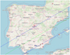 |
Fig. 1 Map of the ground track of our latest prediction update, based on astrometry obtained at the 2 m LT on La Palma. A spherical diameter of D = 285 km was used for 2003 UY117 for the predicted shadow path width (blue lines) plotted in this figure. The map also displays the sites where the occultation was observed, with blue markers indicating a positive detection and red ones indicating a negative detection (i.e., a “miss”). Negative observations reported from Belgium and England, which were located within the uncertainty of the original nominal prediction, are outside this map. Map credit: OpenStreetMap. |
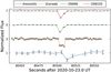 |
Fig. 2 Occultation light curves. The light curves (flux vs. time) are normalized and shifted from each other on the y-axis by an offset value of 2 for clarity. The site, telescope, and instrument details are given in Table A.1. |
2.3 Profile fit
Assuming a spheroidal or an ellipsoidal object, the projected cross section on the sky plane is an ellipse. Therefore, we fit an ellipse to the extremities of the chords (derived from the ingress and egress times as described in Sect. 2.2), taking into account the near misses of the occultation as an additional constraint (Fig. 3). The five solve-for parameters were: the center of the ellipse ( f, g) with respect to the center of the fundamental plane defined by the geocentric star and TNO position for the event time; the semimajor axis, a′; the oblateness, є′ = (a′ − b′)/a′; and the position angle of the ellipse, φ′9. The prime (′) indicates that these parameters belong to the projected (“apparent”) profile ellipse of the object and distinguishes them from the axes of a physical body (triaxial ellipsoid with semiaxes a, b, and c). The parameters were estimated using the Levenberg- Marquardt optimization algorithm. The goodness of the fit was evaluated from the χ2 per degree of freedom (pdf) value, defined as  , where N = 8 is the number of data points and M = 5 is the number of adjustable parameters. Ideally, this value should be close to one. We obtain
  for our fit. The 1σ uncertainties in the retrieved parameters were obtained from a grid search in the parameter space, by varying one parameter from its nominal solution value while keeping the other parameters constant. Acceptable values were those that gave a χ2 between
  . The results of our instantaneous best-fitting limb are summarized in Table 3.
3 Photometry
To interpret the occultation results with respect to the threedimensional shape and size of the physical body, we carried out photometric observations of 2003 UY117 to determine its rotational light curve. We carried out observations with the 1.5 m telescope at Sierra Nevada Observatory (Spain) and with the 1.23 m telescope at Calar Alto Observatory (Spain) over six nights and with longer time coverage than the observations with the 2m LT on La Palma (Sect. 2.1); the latter were done with the IO:O instrument and a Sloan r′ filter, and were focused on astrometry with the aim of updating the occultation prediction. We also used sparse observations made at Calar Alto in 2019 by our group. Observations at the 1.5 m telescope were made with an Andor iKon-L CCD camera (model DZ936N-BEX2-DD)10 without filters in order to increase the signal-to-noise ratio. At the 1.23 m telescope, we used the DLR-MKIII instrument11 (also without filters), except for two nights when we took images with V and R filters to determine the V − R color of the TNO. Image calibration and photometry were performed using the same algorithms and procedures as for the LT images (Sect. 2.1). The science images were calibrated in the usual manner, namely, bias and flat field image correction were applied to them.
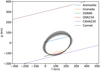 |
Fig. 3 Elliptical fit to the 2020 October 23 occultation observations (chords). This fit describes the limb of 2003 UY117 for the moment of the occultation on the sky plane, defined by the (f, g) axes. As two chords were derived from the same site (OSN90 and OSN150; Sierra Nevada Observatory), they are not distinguishable in the plot. Also shown is the chord for the nearest site to the south (CAHA220: Calar Alto Observatory, 2.2m telescope) and to the north (Cannet), both of which had a negative detection (“miss”). The gray shaded area is the 1σ uncertainty region of the derived ellipse. |
Elliptical occultation limb profile fit result.
3.1 Absolute magnitude
From the calibrated CCD images, we derived magnitudes in the R band using our algorithms that use the Gaia DR2 field stars to determine photometric transformation equations, which take the color information into account (Morales et al. 2022). For the color of the TNO, we used a value of V − R = 0.46 ± 0.07 mag, which was derived from two nights of observations with the Calar Alto 1.23 m telescope. From a linear regression of the reduced R magnitude (the apparent magnitude that the TNO would have at 1 au from the Sun and Earth) at several phase angles, α, we obtained the absolute magnitude, HR = mR(1,1,0), and the phase slope, β (Fig. 4). From the fitted trend line, we derived an absolute magnitude of HR = 5.45 ± 0.01 mag and a slope parameter of β = 0.22 ± 0.01 mag/°. Our observations covered the phase angle range α = [0.118°, 1.638°]. The scatter around the trend line indicates a significant rotational modulation.
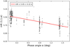 |
Fig. 4 Reduced magnitude mR (1, 1, α) vs. the phase angle, α. In total, 431 observations obtained with the 2 m LT, with the 1.5 m telescope at Sierra Nevada Observatory, and with the 1.23 m telescope at Calar Alto Observatory were used. The brightness variation cluster is due to the rotation of 2003 UY117. |
3.2 Rotational light curve
After de-trending12 the reduced and light-travel-time-corrected photometry, we performed a search for the rotation period of 2003 UY117 using different period-finding techniques. In total, we had more than 400 observations from 2019 November 30 to 2021 February 15. We used the Lomb-Scargle (LS; Lomb 1976; Scargle 1982) algorithm to estimate the most likely rotation period from our data. The algorithm works in the frequency domain, and the most prominent light curve frequencies (in units of 1/day as the timescale of the data is days) are shown in the LS periodogram (Fig. 5). The normalized spectral power reveals a frequency of about 4/day (the exact value is f = 3.878329) as the dominant frequency. Given that a small (ellipsoidal) body typically executes two light curve periods in a single rotation period, the most likely rotation frequency is f = 3.878329/2 (day−1), which corresponds to a rotation period of P = 12.3765 h.
To further constrain and verify the rotation period, we folded the data with a period in the range 4–30 h in 0.00001 day steps. For each period value, we fit a second-order Fourier series to the folded data and calculated the root mean square error (RMSE; Fig. 6). Additionally, we verified the phased plots for the most prominent periods that were derived in both approaches, and we also evaluated split-halves plots. The period with the smallest RMSE is P = 12.3763 h, which we chose as our best estimate for the rotation period of 2003 UY117. The second prominent minimum at 16.692 h (Fig. 6) corresponds to 2.8756 cycles/day, which is a 24h alias of the 1.9392 cycles/day frequency that corresponds to our preferred period of 12.376 h. The periodogram in cycles/day (Fig. 5) in addition to the periodogram in hours helps to identify 24 h aliases of the main peak, which are usually separated by ~ 1 cycle/day. From the results of the two approaches, we conclude that the rotation period is P = 12.376 ± 0.0033 h13. From the best Fourier fit (Fig. 7), we derived a peak-to-valley amplitude of ∆m = 0.36 ± 0.13 mag.
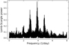 |
Fig. 5 LS periodogram. The rotational light curve frequency is given in 1/day. These values are light curve frequencies (periods); since a small body typically executes two light curve periods in a single rotation period, the best rotation period we obtain from the LS analysis is P = 12.3765 h. |
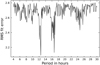 |
Fig. 6 Fourier fit periodogram. We scanned the period range 4–30 hours in 0.00001 h steps, folded the photometric data with the selected period, and fit a second-order Fourier series to the data. The best period we obtained, P = 12.3763 h, is the value for which the RMS of the residuals (data minus fit) reaches a minimum. |
4 Results
4.1 Size and shape
The instantaneous occultation ellipse limb fit to the projected profile of 2003 UY117 (Fig. 3) yields a′ = 141 ± 9 km, b′ = 94 ± 16 km, and φ′ = −31o ± 11o with a  value (Table 3). Given the large amplitude of the rotational light curve, we can expect that the intensity variations are due to shape effects, and this implies that 2003 UY117 is not a spheroid. We assumed that a triaxial ellipsoid with semiaxes a > b > c (spin-axis c) is a good approximation for the physical body. In the following, we deduce the possible shape and size of this ellipsoid from the occultation observation combined with our light curve results. Using the Maclaurin sequence equations (Chandrasekhar 1969), a hydrostatic equilibrium body rotating at ~12 h down to a density of ρ ~ 0.2 g/cm3 would have taken on a Maclaurin spheroid shape, but 2003 UY117 clearly does not have an (oblate) spheroid shape. Valid triaxial ellipsoids in hydrostatic equilibrium (Jacobi solutions) are possible only for densities ranging from 0.254 g/cm3 to 0.333 g/cm3 given the rotation period of 12.38 h. These densities are too low to be realistic for bodies in this size range.
The orthogonal projection of a triaxial ellipsoid (axes a > b > c, rotating around c) for a given spin state, expressed by the aspect angle, ψ (i.e., the angle between the rotation axis, c, and the line of sight) and the rotational phase, ϕ, is (e.g., Magnusson 1986)
 (2)
(2)
 (3)
(3)
 (4)
(4)
 (5)
(5)
where (a′, b′) are the projected semiaxes that correspond to the apparent semiaxes of the projected cross section of an ellipsoidal object during a stellar occultation. The rotational light curve amplitude for such an ellipsoid can be calculated as (e.g., Binzel et al. 1989, p. 426)
 (6)
(6)
By performing a grid search for the three body semiaxes, a, b, and c, and the polar aspect angle, ψ, using the rotational phase angle, ϕ, for the observed occultation time, we can find the best fit to the projected shape derived from the occultation while simultaneously fitting the rotational light curve amplitude (∆m). The rotational phase at the time of the observed 2020 October 23 occultation was ~0.63, measured from the absolute maximum of brightness (Fig. 7). The observed peak-to-valley amplitude is ∆m = 0.36 ± 0.13 mag. We defined the cost function to be minimized as χ2 = (0.36 − ∆mc)2/0.132 + (1.5 − a′/b′)2/0.352 + (141 − a′)2/92, with the modeled light-curve amplitude, ∆mc, derived by Eq. (6), and the apparent semiaxes a′, b′ as obtained from Eqs. (4)–(5) for each triaxial ellipsoid “clone” (defined by a, b, c, and ψ; ϕ = 0.63 ⋅ 2π) created during the grid search. The scanned parameter space was c = [60,120] km, b = [c, 160] km, and a = [b, 200] km, with a grid spacing of 2 km. The aspect angle, ψ, was scanned between 0 and 90 degrees in 1° steps. From this search, we obtained a family of possible solutions of triaxial ellipsoids and aspect angles. The model that minimizes χ2 has axes a = 166 ± 12 km, b = 108 ± 12 km, and  , with an aspect angle of
  . The diameter (of an equal-volume sphere) for this solution is Deq = 235 ± 25 km. The 1σ uncertainties in the retrieved parameters were obtained by varying one parameter from its nominal solution value with corresponding
  , while keeping the other parameters constant.
The spin axis orientation for this object is currently unknown. But if the pole orientation (αp , δp) is known, the aspect angle can be computed as
 (7)
(7)
where α, δ are the coordinates of the object for the date of interest (e.g., the occultation date). By means of a grid search over the whole parameter space in 1° steps, we obtained a pole orientation of (αp, δp) = (337° ± 10°, 62° ± 5°).
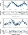 |
Fig. 7 Phased rotational light curve for 2003 UY117 using all the photometric data folded with a period of P = 12.376 h (upper panel) and P = 16.692 h (lower panel). The P = 12.376 h is our preferred solution. This double-peaked light curve with an amplitude of 0.36 mag indicates a highly nonspherical body with a presumable triaxial shape. Phase 0.0 corresponds to the moment of mid-occultation for the observed occultation chords. |
4.2 Absolute magnitude and albedo
From our photometric observations, we obtained an absolute magnitude of HR = 5.45 ± 0.01 mag and a phase slope coefficient of β = 0.22 ± 0.01 mag/° for 2003 UY117 (Fig. 4). Taking into account the brightness contribution due to the rotational phase at the occultation time (about 0.06 mag), and using a color value V − R = 0.46 ± 0.07 mag, which we got from our observations as well, this yields HR = 5.51 ± 0.01 mag and HV = 5.97 ± 0.07 mag. Our V − R value is slightly smaller than the V − R value of 0.56 ± 0.01 mag reported by Sheppard (2012) and the V − R = 0.59 ± 0.01 mag reported by Tegler et al. (2016). Sheppard and Tegler derived absolute magnitudes of HR = 5.35 ± 0.03 mag and HV = 5.91 mag, respectively. Taking into account the large light curve amplitude (which was not considered in the estimates derived by these authors), their values are compatible with ours within the error bars. Our result also agrees with the values of HR = 5.60 ± 0.04 mag, HV = 6.13 ± 0.04 mag, and V − R = 0.53 ± 0.06 mag obtained by Alvarez-Candal et al. (2019), where a half rotational light curve amplitude value of ∆m/2 = 0.06 mag was also considered in the parameter estimation. By applying Eq. (1) with the values D0 = 1330.2 km, Deq,A = 228 ± 21 km as area-equivalent diameter, and HV = 5.97 ± 0.07 mag, we get a geometric albedo of pV = 0.139 ± 0.027 for 2003 UY117.
4.3 Astrometry
The ellipse center coordinates given in Table 3, (119 ± 7, −10 ± 8) km, are two of the five solve-for parameters of the ellipse fit and represent the offset (O-C) between the observed and the predicted position (defined by the object ephemeris and the star position). This information was used to calculate the object position. We derived an astrometric place (ICRS14) for 2003 UY117 at 22:19:21.8 UT on 2020 October 23 with equatorial coordinates

This high-precision astrometry will be used in our orbit determination of the TNO and will also improve the accuracy of future occultation predictions.
5 Conclusions
A stellar occultation by TNO (143707) 2003 UY117 has been predicted and successfully observed for the first time. From four occultation chords observed at three different sites, we derived an instantaneous projected elliptical size of the object with dimensions (282 ± 18) × (184 ± 32) km. The area-equivalent diameter is Deq,A = 228 ± 21 km.
We also obtained the absolute magnitude, phase slope, V − R color, and rotation period for this TNO from our photometric observation campaign. Our preferred rotation period, P, is 12.376 ± 0.0033 hours. The light curve is double-peaked with a peak-to-valley amplitude of ∆m = 0.36 ± 0.13 mag. We obtained an absolute magnitude of HR = 5.51 ± 0.01 mag and HV = 5.97 ± 0.07 mag using a V − R = 0.46 ± 0.07 mag value, which was also derived from our observations. From the area-equivalent diameter of Deq,A = 228 ± 21 km and the absolute magnitude, HV, given above, we derived a geometric albedo of pV = 0.139 ± 0.027.
By combining the occultation with the rotation light curve results, we derived tight constraints on the three-dimensional size and shape of 2003 UY117. Our best solution is 2a = 332 ± 24 km, 2b = 216 ± 24 km, and
 for a triaxial body, which yields an equivalent spherical diameter of Deq = 235 ± 25 km. This value is slightly larger than the radiometric result
  (Farkas-Takács et al. 2020), but well within the error margins. The aspect angle we derived for the occultation epoch is
  . A pole solution that is compatible with the findings above is (αp, δp) = (337° ± 10°,62° ± 5°).
We derived an occultation-based astrometric position (ICRS) for 2003 UY117.
Acknowledgements
Part of this work was supported by the Spanish projects PID2020-112789GB-I00 from AEI and Proyecto de Excelencia de la Junta de Andalucía PY20-01309. Authors J.L.O., P.S-.S., N.M., M.V.-L., and R.D. acknowledge financial support from the Severo Ochoa grant CEX2021-001131-S funded by MCIN/AEI/ 10.13039/501100011033. PS-S also acknowledges financial support from the Spanish I+D+i project PID2022-139555NB-I00 (TNO- JWST) funded by MCIN/AEI/10.13039/501100011033. A.A-.C. acknowledges financial support from the Severo Ochoa grant CEX2021-001131-S funded by MCIN/AEI/10.13039/501100011033. J.I.B.C. acknowledges grants 305917/20196, 306691/2022-1 (CNPq) and 201.681/2019 (Rio de Janeiro State Research Support Foundation, FAPERJ). This work is partly based on observations collected at the Centro Astronómico Hispano en Andalucía (CAHA) at Calar Alto, operated jointly by Junta de Andalucía and Consejo Superior de Investigaciones Científicas (CSIC). This research is also partially based on observations carried out at the Observatorio de Sierra Nevada (OSN) operated by Instituto de Astrofísica de Andalucía (IAA-CSIC) and on observations made with the Liverpool Telescope (LT) at the Roque de los Muchachos Observatory (ORM) on the island of La Palma as part of the Observatorios de Canarias (OCAN) operated by the Instituto de Astrofísica de Canarias (IAC). This study was financed in part by the Coordenação de Aperfeiçoamento de Pessoal de Nível Superior – Brasil (CAPES) – Finance Code 001 and National Institute of Science and Technology of the e-Universe project (INCT do e-Universo, CNPq grant 465376/2014-2). FBR acknowledges CNPq grant 316604/2023-2. ˙İST60 and ˙İST40 are the observational facilities of the Istanbul University Observatory which were funded by the Scientific Research Projects Coordination Unit of Istanbul University with project numbers BAP-3685 and FBG-2017-23943 and the Presidency of Strategy and Budget of Republic of Turkey with the project 2016K12137. We acknowledge all observers which might have tried to observe this occultation event and which are not mentioned explicitly in Table A.1.This work has made use of data from the European Space Agency (ESA) mission Gaia 15, processed by the Gaia Data Processing and Analysis Consortium (DPAC)16. Funding for the DPAC has been provided by national institutions, in particular the institutions participating in the Gaia Multilateral Agreement. We thank the referee and editor for their valuable comments, which helped us to improve the quality and readability of the manuscript. This research has made use of the CORA web portal17.
Appendix A Additional table
Observation details for the 2020 October 23 occultation.
References
- Alvarez-Candal, A., Ayala-Loera, C., Gil-Hutton, R., et al. 2019, MNRAS, 488, 3035 [NASA ADS] [CrossRef] [Google Scholar]
- Binzel, R. P., Gehrels, T., & Matthews, M. S. 1989, Asteroids II (Tucson: University of Arizona Press) [Google Scholar]
- Braga-Ribas, F., Sicardy, B., Ortiz, J. L., et al. 2014, Nature, 508, 72 [NASA ADS] [CrossRef] [Google Scholar]
- Chandrasekhar, S. 1969, Ellipsoidal Figures of Equilibrium (New Haven and London: Yale University Press) [Google Scholar]
- Desmars, J., Camargo, J. I. B., Braga-Ribas, F., et al. 2015, A&A, 584, A96 [NASA ADS] [CrossRef] [EDP Sciences] [Google Scholar]
- Farkas-Takács, A., Kiss, Cs., Vilenius, E., et al. 2020, A&A, 638, A23 [NASA ADS] [CrossRef] [EDP Sciences] [Google Scholar]
- Ferreira, J. F., Tanga, P., Spoto, F., Machado, P., & Herald, D. 2022, A&A, 658, A73 [NASA ADS] [CrossRef] [EDP Sciences] [Google Scholar]
- Gault, D., Nosworthy, P., Nolthenius, R., Bender, K., & Herald, D. 2022, Minor Planet Bull., 49, 3 [Google Scholar]
- Gomes-Júnior, A. R., Morgado, B. E., Benedetti-Rossi, G., et al. 2022, MNRAS, 511, 1167 [CrossRef] [Google Scholar]
- Harris, A. W. 1998, Icarus, 131, 291 [Google Scholar]
- Horner, J., Evans, N. W., & Bailey, M. E. 2004, MNRAS, 354, 798 [NASA ADS] [CrossRef] [Google Scholar]
- Hubbard, W. B., Hunten, D. M., Dieters, S. W., Hill, K. M., & Watson, R. D. 1988, Nature, 336, 452 [NASA ADS] [CrossRef] [Google Scholar]
- Kaminski, K., Weber, C., Marciniak, A., Zolnowski, M., & Gedek, M. 2023, PASP, 135, 025001 [CrossRef] [Google Scholar]
- Kervella, P., Thévenin, F., Di Folco, E., & Ségransan, D. 2004, A&A, 426, 297 [NASA ADS] [CrossRef] [EDP Sciences] [Google Scholar]
- Kilic, Y., Braga-Ribas, F., Kaplan, M., et al. 2022, MNRAS, 515, 1346 [NASA ADS] [CrossRef] [Google Scholar]
- Leiva, R., Buie, M. W., Keller, J. M., et al. 2020, Planet. Sci. J., 1, 48 [NASA ADS] [CrossRef] [Google Scholar]
- Lellouch, E., Santos-Sanz, P., Lacerda, P., et al. 2013, A&A, 557, A60 [NASA ADS] [CrossRef] [EDP Sciences] [Google Scholar]
- Lomb, N. R. 1976, Astrophys. Space Sci., 39, 447 [Google Scholar]
- Magnusson, P. 1986, Icarus, 68, 1 [NASA ADS] [CrossRef] [Google Scholar]
- Morales, N., Ortiz, J. L., Morales, R., et al. 2022, Europlanet Science Congress 2022, EPSC2022-664 [NASA ADS] [Google Scholar]
- Müller, T. G., Lellouch, E., Böhnhardt, H., et al. 2009, Earth Moon Planet, 105, 209 [CrossRef] [Google Scholar]
- Nesvorný, D., & Morbidelli, A. 2012, AJ, 144, 117 [Google Scholar]
- Oliveira, J. M., Sicardy, B., Gomes-Júnior, A. R., et al. 2022, A&A, 659, A136 [NASA ADS] [CrossRef] [EDP Sciences] [Google Scholar]
- Ortiz, J. L., Duffard, R., Pinilla-Alonso, N., et al. 2015, A&A, 576, A18 [NASA ADS] [CrossRef] [EDP Sciences] [Google Scholar]
- Ortiz, J. L., Santos-Sanz, P., Sicardy, B., et al. 2017, Nature, 550, 219 [NASA ADS] [CrossRef] [Google Scholar]
- Rieke, G. H., Blaylock, M., Decin, L., et al. 2008, AJ, 135, 2245 [NASA ADS] [CrossRef] [Google Scholar]
- Rommel, F. L., Braga-Ribas, F., Desmars, J., et al. 2020, A&A, 644, A40 [NASA ADS] [CrossRef] [EDP Sciences] [Google Scholar]
- Russell, H. N. 1916, ApJ, 43, 173 [Google Scholar]
- Santos-Sanz, P., Lellouch, E., Fornasier, S., et al. 2012, A&A, 541, A92 [NASA ADS] [CrossRef] [EDP Sciences] [Google Scholar]
- Sarid, G., Volk, K., Steckloff, J. K., et al. 2019, ApJ, 883, L25 [Google Scholar]
- Scargle, J. D. 1982, ApJ, 263, 835 [Google Scholar]
- Sheppard, S. S. 2012, AJ, 144, 169 [NASA ADS] [CrossRef] [Google Scholar]
- Sicardy, B., Widemann, T., Lellouch, E., et al. 2003, Nature, 424, 168 [NASA ADS] [CrossRef] [Google Scholar]
- Tegler, S. C., Romanishin, W., Consolmagno, G. J., & J., S. 2016, AJ, 152, 210 [NASA ADS] [CrossRef] [Google Scholar]
- Willmer, C. N. A. 2018, ApJS, 236, 47 [Google Scholar]
- Zacharias, N., Monet, D. G., Levine, S. E., et al. 2004, Am. Astron. Soc. Meet. Abstr., 205, 48.15 [Google Scholar]
Data retrieved from the MPC on 2024 January 22.
Photodetector Array Camera and Spectrometer.
Numerical Integration of the Motion of an Asteroid.
Stellar Occultation Reduction and Analysis.
The (clockwise positive) angle between the “g-positive” direction (i.e., north) and the semiminor axis, b′.
i.e., using the O-C residuals of the linear fit described in Sect. 3.1.
The 1σ error was derived from the period value differences corresponding to  .
.
International Celestial Reference System.
All Tables
All Figures
|
Fig. 1 Map of the ground track of our latest prediction update, based on astrometry obtained at the 2 m LT on La Palma. A spherical diameter of D = 285 km was used for 2003 UY117 for the predicted shadow path width (blue lines) plotted in this figure. The map also displays the sites where the occultation was observed, with blue markers indicating a positive detection and red ones indicating a negative detection (i.e., a “miss”). Negative observations reported from Belgium and England, which were located within the uncertainty of the original nominal prediction, are outside this map. Map credit: OpenStreetMap. |
| In the text | |
|
Fig. 2 Occultation light curves. The light curves (flux vs. time) are normalized and shifted from each other on the y-axis by an offset value of 2 for clarity. The site, telescope, and instrument details are given in Table A.1. |
| In the text | |
|
Fig. 3 Elliptical fit to the 2020 October 23 occultation observations (chords). This fit describes the limb of 2003 UY117 for the moment of the occultation on the sky plane, defined by the (f, g) axes. As two chords were derived from the same site (OSN90 and OSN150; Sierra Nevada Observatory), they are not distinguishable in the plot. Also shown is the chord for the nearest site to the south (CAHA220: Calar Alto Observatory, 2.2m telescope) and to the north (Cannet), both of which had a negative detection (“miss”). The gray shaded area is the 1σ uncertainty region of the derived ellipse. |
| In the text | |
|
Fig. 4 Reduced magnitude mR (1, 1, α) vs. the phase angle, α. In total, 431 observations obtained with the 2 m LT, with the 1.5 m telescope at Sierra Nevada Observatory, and with the 1.23 m telescope at Calar Alto Observatory were used. The brightness variation cluster is due to the rotation of 2003 UY117. |
| In the text | |
|
Fig. 5 LS periodogram. The rotational light curve frequency is given in 1/day. These values are light curve frequencies (periods); since a small body typically executes two light curve periods in a single rotation period, the best rotation period we obtain from the LS analysis is P = 12.3765 h. |
| In the text | |
|
Fig. 6 Fourier fit periodogram. We scanned the period range 4–30 hours in 0.00001 h steps, folded the photometric data with the selected period, and fit a second-order Fourier series to the data. The best period we obtained, P = 12.3763 h, is the value for which the RMS of the residuals (data minus fit) reaches a minimum. |
| In the text | |
|
Fig. 7 Phased rotational light curve for 2003 UY117 using all the photometric data folded with a period of P = 12.376 h (upper panel) and P = 16.692 h (lower panel). The P = 12.376 h is our preferred solution. This double-peaked light curve with an amplitude of 0.36 mag indicates a highly nonspherical body with a presumable triaxial shape. Phase 0.0 corresponds to the moment of mid-occultation for the observed occultation chords. |
| In the text | |
Current usage metrics show cumulative count of Article Views (full-text article views including HTML views, PDF and ePub downloads, according to the available data) and Abstracts Views on Vision4Press platform.
Data correspond to usage on the plateform after 2015. The current usage metrics is available 48-96 hours after online publication and is updated daily on week days.
Initial download of the metrics may take a while.