| Issue |
A&A
Volume 691, November 2024
|
|
|---|---|---|
| Article Number | A297 | |
| Number of page(s) | 6 | |
| Section | Stellar atmospheres | |
| DOI | https://doi.org/10.1051/0004-6361/202450987 | |
| Published online | 21 November 2024 | |
The variability of Betelgeuse explained by surface convection★
1
Institut de Recherche en Astrophysique et Planétologie, Université de Toulouse, UPS, CNRS,
IRAP/UMR 5277, 14 avenue Edouard Belin,
31400
Toulouse,
France
2
IRAP, Université de Toulouse, CNRS, UPS, CNES,
57 avenue d’Azereix,
65000
Tarbes,
France
★★ Corresponding author; This email address is being protected from spambots. You need JavaScript enabled to view it.
Received:
4
June
2024
Accepted:
8
October
2024
Abstract
Context. Betelgeuse is a red supergiant (RSG) that is known to vary semi-regularly on both short and long timescales. The origin of the short period of Betelgeuse has often been associated with radial pulsations, but could also be due to the convection motions present at the surface of RSGs.
Aims. We investigate the link between surface activity and the variability of the star.
Methods. Linear polarization in Betelgeuse is a proxy of convection that is unrelated to pulsations. Using ten years of spectropolarimetric data of Betelgeuse, we looked for periodicities in the least-squares deconvolution profiles of Stokes I, Q, U and the total linear polarization using Lomb–Scargle periodograms.
Results. We find periods in linear polarization signals that are similar to those in photometric variability. The 400 d period is too close to a peak of the window function of our data, but the two periods of 330 d and 200 d are present in the periodogram of Stokes Q and U, showing that the variability of Betelgeuse can be interpreted as being due to surface convection.
Conclusions. Since the linear polarization in the spectrum of Betelgeuse is not known to vary with pulsations, but is linked to surface convection, and since similar periods are found in the time series of photometric measurements and spectropolarimetry, we conclude that the photometric variability is due to the surface convective structures, and not to any pulsation phenomenon.
Key words: stars: atmospheres / supergiants
Based on observations obtained at the Télescope Bernard Lyot (TBL) at Observatoire du Pic du Midi, CNRS/INSU and Université de Toulouse, France.
© The Authors 2024
 Open Access article, published by EDP Sciences, under the terms of the Creative Commons Attribution License (https://creativecommons.org/licenses/by/4.0), which permits unrestricted use, distribution, and reproduction in any medium, provided the original work is properly cited.
This article is published in open access under the Subscribe to Open model. This email address is being protected from spambots. You need JavaScript enabled to view it. to support open access publication.
1 Introduction
Betelgeuse is a prototypical red supergiant (RSG), known to be a semi-regular variable. Several periods can be found in the literature, usually clustered around the long secondary period (LSP) of 2000 d, plus shorter periods around 400 and 200 d (Kiss et al. 2006). The origin of the LSP remains a source of discussion: some have tried to find the explanation of the LSP in the lifetime of the large convective cells present at the surface of RSGs (e.g Stothers 2010), while others have invoked a magnetic field (Wood et al. 2004). The shorter periods of 400 and 200 d are given a different origin from that of the LSP, and are traditionally attributed to radial pulsation, the 400 d period being the fundamental mode and the 200 d the first overtone (Guo & Li 2002; Joyce et al. 2020). By studying a large sample of RSGs, Kiss et al. (2006) found a period of 388 ± 30 d, which was later confirmed by Chatys et al. (2019). Further works have been carried out to identify periods in Betelgeuse; for instance, using the observations from the AAVSO database between 1995 and 2014, Montargès et al. (2016) found a period of 423.59 ± 39 d. Furthermore, Jadlovský et al. (2023) found a photometric period of 417 ± 17 d, while Joyce et al. (2020) found a period of 416 ± 24 d and identified another shorter period of 185 ± 13.5 d being attributed to the first overtone, in agreement with the historical work of Stothers (1969).
In addition to radial pulsation, surface activity leading to random brightness variation has also been mentioned to explain the variability of Betelgeuse, first theorized by Schwarzschild (1975). More recently, Gray (2008) proposed that the 400 d period was a consequence of convective activity. Betelgeuse is known to present large convective cells with lifetimes on the order of one to two years (López Ariste et al. 2018) and measurable changes within the span of one week. Those typical convective timescales are also seen in numerical simulations of RSGs, where the smallest convective granules live on a timescale of a few weeks to a month and the largest on a timescale of a few months up to a few years (Chiavassa et al. 2022). Bright convection cells near the disk center will increase the integrated brightness of the star compared with other situations where similar cells are found near the edges. So, even without invoking the formation of dust or other changes in opacity, it can be argued that the simple evolution of convective patterns of the star may create variability. This variability could be expected to be random, but will present quasi-periodicities related to the typical timescales of the convective patterns (Gray 2008).
At the end of 2019, Betelgeuse reached a historical minimum in its luminosity called the Great Dimming (Guinan et al. 2020). From interferometric and spectroscopic data, it has been proposed that this event was caused by the formation of a cloud of dust close to the line of sight (Montargès et al. 2021). Interferometric images show a drop in luminosity in the southern hemisphere of Betelgeuse, which could be caused by a mass loss event and lead to this dimming (Dupree et al. 2022). Other hypotheses have also been explored, such as a drop in temperature (Harper et al. 2020), or an increase in the molecular opacity (Kravchenko et al. 2021). In this event, it turns out that a change in brightness was not due to pulsation, but to a change in the brightness distribution over the stellar disk. Since the end of the Great Dimming event, Betelgeuse has continued its random variation in brightness. Quite interestingly, however, it has been shown by Jadlovský et al. (2023) and Dupree et al. (2022) that the periodicity of Betelgeuse has changed since the dimming. Using the light curves from AAVSO, the cited authors showed that before the dimming, the dominant period of Betelgeuse was the 400 d period, while after the Great Dimming, the main periods of Betelgeuse have shortened, oscillating between 97 d and 230 d (Dupree et al. 2022), revealing a change in the behavior of the atmosphere of Betelgeuse. While the Great Dimming may be seen as a singular event, such modifications of the variability periods bring up the question of whether all changes in brightness can be due to similar changes in the brightness distribution over the disk and unrelated to any pulsation phenomenon. Our interest in an alternative explanation of the variability in terms of convective patterns arose. In order to address this question, we seek typical periods of 400 and 200 d in observational proxies related to the convective activity but not to any pulsation, such as the linear polarization spectra.
Linear polarization in the atomic lines of the spectrum of Betelgeuse, discovered by Aurière et al. (2016), has been interpreted as the joint action of two mechanisms. The first is the depolarization of the continuum by atoms that absorb linearly polarized light from the continuum and re-emit unpolarized light, the continuum photons being polarized by Rayleigh scattering. This depolarization produces signals with azimuthal symmetry over the visible disk, which would cancel out the net linear polarization on a homogeneously bright disk. Thus, such a mechanism of polarization must be combined with an inhomogeneously bright disk to produce the net linear polarization signal observed. This interpretation suggests the possibility of mapping those brightness inhomogeneities. This has been achieved by López Ariste et al. (2018), who produced three-dimensional images of the atmosphere of Betelgeuse (López Ariste et al. 2022) by taking advantage of the different heights of formation of different lines in the spectrum of Betelgeuse. The produced images compare very well with contemporaneous images made with interferometric techniques (Montargès et al. 2016) and show clear convective patterns, similar to solar granulation.
Linear polarization observed in the atomic lines is therefore a proxy of convection, unrelated a priori to radial pulsations, but linked to the brightness inhomogeneities due to the convective patterns in Betelgeuse. If we can find the aforementioned variability periods in linear polarization, we can conclude that these periods are related to the convective activity that originates the linear polarization signals. This is the purpose of the present work.
In Sect. 2, we describe the dataset of linear polarization obtained with Narval and Neo-Narval at the two-meter Télescope Bernard Lyot (TBL), as well as the Lomb–Scargle periodograms used to derive periods. In Sect. 3, we seek periods in the least-squares deconvolution (LSD) profiles of Betelgeuse using the Lomb–Scargle periodogram. In Sect. 4, we associate the 200 d period with the convective timescale of the smallest granules and the 330 d periodicity with the largest granules. We speculate on an explanation in the change of variability of Betelgeuse before and after the Great Dimming.
2 The polarimetric data
Betelgeuse has been observed since 2013 with Narval and Neo-Narval at the Télescope Bernard Lyot1. The polarimeter Narval observed Betelgeuse on average every month from November 2013 to April 2019, except during the summer, representing a total of 56 observations over 5.5 years. During this period, Betelgeuse was observed 43% of the time between January and April and 57% between September and December. Before the Great Dimming of Betelgeuse, Narval was replaced by Neo-Narval, which has been observing Betelgeuse since early 2020. These two instruments measure the polarization over the visible and near infrared spectra of Betelgeuese (390–1000 nm) with high spectral resolution (R = 65 000) and high polarimetric sensitivity. The signal-to-noise ratios are not sufficient to measure the weak polarization signals in individual atomic lines of the spectrum. These amplitudes are known to be on the order of 10−4 times the continuum intensity, and they only exceptionally reach amplitudes of 10−3. When these high amplitudes are present, enough photons can be accumulated per spectral bin to detect the linear polarization signal above noise in lines (Aurière et al. 2016). Usually, the amplitudes of linear polarization are below noise levels. On those occasions, we have to add up the signals of thousands of lines to increase the signal-tonoise ratios. This addition is performed through the LSD (Donati et al. 1997; Kochukhov et al. 2010). This technique has been successfully used in the past to measure magnetic field distributions over stellar surfaces (e.g Donati & Landstreet 2009; Reiners 2012; Kochukhov 2021) and is now employed to produce images of the brightness distributions in the photosphere of Betelgeuse and other RSGs, as cited in Sect. 1. To produce the LSD profiles, we used a solar abundance line mask, similar to the one used by Aurière et al. (2016) and Mathias et al. (2018), which was calculated from the data provided by VALD (Kupka et al. 1999), for an effective temperature of 3750 K, log g = 0.0 and a microturbulence of 4 km s−1, aligning with the physical parameters of Josselin & Plez (2007). The mask includes approximately 15 000 lines with depths exceeding 40% of the continuum.
In this work, we examine the signals produced through the LSD technique, which in turn produce a pseudo-spectral line in intensity and linear polarization. This pseudo-spectral line does not correspond to any particular atomic species, but rather represents an average of all species present and emitting in the photosphere of Betelgeuse. Following these procedures of line addition, the resulting profiles carry the coherent signals present in the photospheric lines, but the specific characteristics of individual spectral lines are erased. All of this data has been presented by Aurière et al. (2016), Mathias et al. (2018), and López Ariste et al. (2022), who also provide details on observing times and conditions as well as a more detailed description of the data reduction process2.
We note that all the velocities mentioned in the text or in the figures are provided in the heliocentric frame.
3 Period search
Anyone attempting to identify periods in an astrophysical context faces the challenge of unevenly spaced observed data. To overcome this hurdle, we used the Lomb–Scargle periodogram (Lomb 1976; Scargle 1982) as implemented in astropy (Astropy Collaboration 2018). This method involves fitting sinusoids to the data using least-squares with the frequency sampled between the first and last observation. The quality of the fit determines the power attributed to a frequency. We applied this technique to the LSD profiles of Stokes I, Q, U, and to the total linear polarization of Betelgeuse observed by the TBL with Narval from 2013 to 2019, with a total of 56 observations. We also looked at the periodograms obtained from the dataset available post-dimming, from 2020 to 2024. However, the base time of this dataset is not long enough to produce meaningful periodograms. Therefore, our focus was on periodograms computed exclusively from data obtained before the Great Dimming with Narval.
3.1 Variability of the Stokes parameters
We first computed the Lomb–Scargle periodogram at each wavelength of the LSD profile, ranging from −25 km s−1 to +60 km s−1 with a step of 1.8 km s−1 to cover the entire signal present in the LSD profile. López Ariste et al. (2018) identified the most blueshifted signal towards −20 km s−1 and interpreted it as the maximum velocity of the rising plasma. The most redshifted signal was often found at +40 km s−1, interpreted as the rest velocity of the star. Sometimes, signals at velocities greater than +40 km s−1 can be found, with a peak in the linear polarization signal up to 50 km s−1 (López Ariste et al. 2022), which can be interpreted either as dark and cold plasma falling back to Betelgeuse or as rising plumes of plasma located on the hidden face of Betelgeuse, ascending so high that they appear above the limb (López Ariste et al. 2023, for the case of the RSG μ Cep). The +60 km s−1 limit in the Lomb–Scargle periodograms was set to include the occasional linear polarization peaks beyond the velocity of the star.
Figures 1–4 show the Lomb–Scargle periodogram of the LSD profile for Stokes I, Stokes Q, Stokes U, and the total linear polarization, respectively. In each figure, the upper panel depicts the Lomb–Scargle periodogram of each velocity bin (gray lines) along with the total average (red line). The green line represents the window function. The spectral window reflects the pattern caused by the structure of gaps in the time sampling. The peaks pointed out by this window cannot be interpreted as ones related to the star. The lower panel shows the Lomb–Scargle periodogram for each velocity bin, with the white dotted lines marking the 400 and 200 d periods for reference. The right panel represents the mean profile of each Stokes parameter at each velocity bin.
Figure 1 shows the Lomb–Scargle periodogram of the LSD of the intensity profile; we observe that the 400 and 200 d periods seem to be captured by the periodogram. However, the 400 d period is uncomfortably close to the peak of the window function. Furthermore, both periods are located at the same HRV and in the blue wing of the profile. Interestingly, Mathias et al. (2018) previously found this 200 d periodicity in spectroscopic observation, despite a shorter observation period.
Figures 2 and 3 display the Lomb–Scargle periodograms of Stokes Q and U. These periodograms exhibit significant differences compared to the intensity periodogram. In Fig. 2 a prominent signal is evident around 200 d. Regarding Stokes U in Fig. 3, it appears that the primary frequency is approximately 0.003 d−1 (equivalent to a 330 d period). Other periods, such as those at 200 d or 250 d (0.004 d−1) are present, but are difficult to trust. From both periodograms of Stokes Q and U, we recover the 200 d period, and also the 330 d period is notable, which aligns closely with the 400 d period reported in the literature and is in agreement with the timescale of the hysteresis loop reported by Kravchenko et al. (2019). Figure 4 shows the Lomb–Scargle periodogram of ![Mathematical equation: $\[\sqrt{Q^{2}+U^{2}}\]$](/articles/aa/full_html/2024/11/aa50987-24/aa50987-24-eq1.png) , representing the total linear polarization of Betelgeuse. This periodogram confirms the significant powers at both 330 d and 200 d, consistent with the periodograms of Stokes Q and U.
, representing the total linear polarization of Betelgeuse. This periodogram confirms the significant powers at both 330 d and 200 d, consistent with the periodograms of Stokes Q and U.
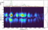 |
Fig. 1 Lomb–Scargle periodogram of the LSD profile of intensity. The upper panel is the Lomb–Scargle periodogram for each velocity bin (gray lines) and the average (red line). The green line is the window function. In the lower panel, the two white dashed lines mark respectively the 400 d and the 200 d periods. The y-axis represents the heliocentric radial velocity (HRV). The color axis marks the power of the fit: red shows a higher power than dark blue. The right panel is the average intensity profile for each velocity bin. |
![Mathematical equation: $\[\sqrt{Q^{2}+U^{2}}\]$](/articles/aa/full_html/2024/11/aa50987-24/aa50987-24-eq2.png)
3.2 Variability of the polarimetric imaging
Using linear polarization, López Ariste et al. (2018) successfully reconstructed images of Betelgeuse, which have been compared favorably to inteferometric images obtained by Montargès et al. (2016). The images were produced by finding the brightness distribution that best fits the observed linear polarization LSD profile using a Marquardt-Levenberg minimization.
Betelgeuse is observed, on average, every month by the TBL, enabling the tracking of its surface activity through this technique of polarimetric imaging. This technique has previously allowed the estimation of the size and the lifetime of convective cells on the surface (López Ariste et al. 2018). From these images, we computed a photo-center, a quantity sensitive to the size and number of convective cells. The photo-center was computed from Eqs. (2) and (3) given by Chiavassa et al. (2022). A homogeneous star will have a photo-center displacement coinciding with the barycenter of the star, whereas a star with one or two large convective cells will exhibit a more significant photocenter displacement, up to a few percent of the stellar radius in the case of RSGs (Chiavassa et al. 2022).
Since the photo-center is linked to surface convection, it is worth checking for periods in its dynamics over the five years of observations of Betelgeuse before the dimming. While these periods may overlap with those presented in the previous section, they are likely to capture additional aspects of the phenomena at work. However, before proceeding to search for periods in the displacement of the photo-center, it is important to address a key issue regarding the interpretation of these images. Linear polarization suffers from a 180° degree ambiguity, as mentioned in Aurière et al. (2016). Consequently, our images can be rotated by 180° degree, and the brightness distribution will still fit the observed LSD polarization profiles. If each observation were treated independently, the algorithm’s solution could be any of the possible ambiguous solutions. To ensure continuity between the image series, for a given day, we use the brightness distribution of the previous day as the initial point of the fitting iteration. The first image in the series begins its minimization iteration with a random brightness distribution. Although we can produce a series of consistent images, it is important to keep in mind that the photo-center displacement computed from the series will be affected by the initial image. To overcome this issue, we compute the photo-center displacement from 100 different time series, each starting from a different initial image. This approach aims to recover ensemble properties independent of the choice of the first image.
Figure 5 shows the Lomb–Scargle periodogram of the photocenter displacement for each of the 100 series (blue lines) and the average Lomb–Scargle periodogram (black line). The red dashed lines indicate the 400 and 200 d periods, respectively. The black horizontal line represents the 1σ confidence level, which was computed from the standard deviation of the average Lomb-Scarlge periodogram. As in the previous figures, the window function is represented by the green line. Interestingly, we find two peaks around the 400 d period in the periodogram, one at 0.0024 d−1 and one at 0.003 d−1, that are above the 1σ confidence level. Although they are not individually significant to confirm the presence of a similar period, these peaks are consistent with the findings described in the previous section. Since polarimetry imaging involves only surface convection, this provides further support for a variability being explained by surface convection alone.
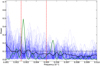 |
Fig. 5 Lomb–Scargle periodogram of the 100 photo-center displacement series of Betelgeuse. Each blue line corresponds to a Lomb–Scargle periodogram of one photo-center displacement. The black line is the average of the 100 periodograms. The red dashed lines represent the 400 and 200 d period, respectively. The green line is the window function. The black horizontal line marks the 1σ confidence level. |
3.3 Variability of the light curve
After examining the periods identified by the Lomb–Scargle technique in the polarization data obtained by the TBL over the last years before the dimming, it is worth contextualizing them alongside the periods traditionally identified in light curves over the same period of time. Two aspects are of interest to us in this comparison: the behavior of the light curve before and after the Great Dimming.
We retrieved the light curve of Betelgeuse in the visible from the AAVSO database for the past ten years. It is shown in Fig. 6. Before the Great Dimming, Betelgeuse’s magnitude exhibited variations on a yearly timescale, whereas after the dimming its variability has shortened. Figure 6 clearly illustrates that the variability of Betelgeuse now occurs on a timescale shorter than one year. This qualitative change has been pointed out before; before the Great Dimming the primary period of Betelgeuse was approximately 400 d (Kiss et al. 2006), often associated with the fundamental pressure mode. However, after the dimming this period seems to have vanished, and only timescales shorter than 230 d are visible (Dupree et al. 2022). No explanations have been put forth regarding this change in variability after, or perhaps because of, the dimming.
In Fig. 7, the upper panel is the periodogram of the mean intensity profile (red line) shown in Fig. 1. In the middle panel, we computed the periodogram from the light curve of Betelgeuse from 1990 to 2024, represented with the blue line. The orange line in the lower panel depicts the periodogram computed exclusively with AAVSO observations made less than two days from our observation dates of the TBL, representing a total of 28 observations. In every panel, the green line represents the window function. For the periodogram since 1990, we binned the observations with intervals of ten days, as Betelgeuse has been observed more often in the 21st century (Kiss et al. 2006). This periodogram recovers the 400 d period and also a period close to 200 d. Other visible peaks are instead due to the windowing effect. When focusing on the periodogram derived from the light curve corresponding to the TBL observation dates (lower panel), we recover the 400 d period, which is once again very close to a peak of the window function. A smaller peak is also present around 200 d. The comparison between this periodogram and the one obtained from Stokes I is important to validate our results. Stokes I is linked to the total amount of light, that is the light curve. Hence, by taking observations of the AAVSO that correspond to the TBL observation dates of Betelgeuse, we should recover the same periods as those found in the Stokes I periodogram. Since we found the 400 d and the 200 d periods in both periodograms, this validates our results. In both cases the peak at 400 d is too close to a peak of the window function to be interpreted as a real peak. On the other hand, the second peak around 200 d could be interpreted as a real peak. In the future, extended spectropolarimetric observations of Betelgeuse will be necessary to smooth the window function of the TBL, and perhaps disentangle the 400 d period from the window function.
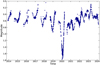 |
Fig. 6 Light curve of Betelgeuse from AAVSO in the V-band. |
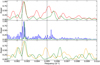 |
Fig. 7 Spectroscopy vs. Photometry periodograms. Upper panel: Lomb–Scargle periodogram of the mean intensity profile presented in Fig. 1 (red line). Middle panel: periodogram of the light curve since 1990 as retrived from the AAVSO database (blue line). Lower panel: periodogram of the light curve (orange line) from AAVSO when the dates correspond to the TBL observations. In every panel, the green line marks the associated window function. The 400 d and the 200 d periods are marked by the black dashed lines. |
4 Discussion
The presence of the same periods in the periodogram derived from the AAVSO and those obtained from linear polarization, considering the time span and sparsity of the TBL data series, point to a common origin, which seems to be based upon convective dynamics. Since we associate Stokes Q and U with proxies of convection, we associate the 200 d period with the typical timescales on which the Stokes parameters evolve. The LSD profiles of Stokes Q or U undergo slight changes when observing Betelgeuse monthly, but are completely overhauled on timescales of several months. The Lomb–Scargle periodograms seem to capture this spectral dynamic at periods of approximately 200 d. These changes in the profiles are directly linked to the dynamics of the surface, to the evolution, and to movements of convective cells across the visible hemisphere. Therefore, the 200 d period appears to be related to the evolution of the convective patterns on the surface of Betelgeuse. The stronger presence of this peak in Stokes Q compared to U was already pointed out by Mathias et al. (2018), and could be interpreted as a temporal situation of how convective patterns have been distributed in the last years.
The other period found in the total linear polarization and Stokes U, the 330 d periods, is not so far from the 400 d period often mentioned in the literature (e.g. Kiss et al. 2006 found a period of 388 ± 30 d). It has been shown by López Ariste et al. (2018) that large convective cells can persist for one to two years. Thus, the 330 d period could be associated with the timescale on which the largest granules evolve. This characteristic timescale has also been observed in the numerical simulations, and might play an important role in determining stellar distances through the displacement of the photo-center (Chiavassa et al. 2022). Once again, we observe the 330 d periodicity to be more prominent in Stokes U than in Q, which may unravel a random situation due to convective motions in the last years. Convective cells could arise in peculiar positions, where the Stokes U profile remains unchanged for months, but where Stokes Q could change on shorter timescales. This interpretation aligns with the work of Gray (2008), who attributed the 400 d period to large convective cells. Whether this 330 d period and the commonly cited 400 d period are one and the same will have to wait for extended spectropolarimetric observations with the TBL that smooth the windowing function around these frequencies.
Regarding the Stokes I profile, a peak closer to the 400 d period appears, but is once again uncomfortably close to a peak of the window function of the TBL, making it difficult to trust. A secondary peak close to 200 d is also present in the Stokes I profile, that we fully assimilate to the one found in the Stokes parameters, and that we attribute to convective timescales.
Before summing up the results of our work, we would like to propose an explanation for the variability of Betelgeuse after the Great Dimming with surface convection. RSGs experience mass loss events, where plasma is ejected into the interstellar medium (Josselin & Plez 2007). These events have been inferred in RSGs, for example μ Cep at photospheric heights, where López Ariste et al. (2023) found an excess of linear polarization beyond the limb of the star, attributing it to rising plumes of plasma in the back hemisphere of the star. In the case of Betelgeuse, the excess of linear polarization beyond the limb is rare and not as pronounced as those observed in μ Cep. They do not appear to contribute to the variability of the star. However, since the Great Dimming, the variability of Betelgeuse has changed. This suggests that the Great Dimming differed significantly from the usual mass loss event, that it disrupted the dynamics of the photosphere.
In a scenario where the variability of Betelgeuse is primarily governed by convection, the visible periods of such variability were associated, before the Great Dimming, with the typical timescales at which convection occurs: approximately 200 d for the small structures and roughly 350 d for the large structures. The Great Dimming affected the behavior of the photosphere in such a way that the largest structures no longer evolved on a timescale around 350 d, but rather on the shorter timescales of the smallest convective structures, around 200 d. We hypothesize that since the Great Dimming event, the photosphere has not yet returned to equilibrium, and the largest convective structures have been disrupted by the turbulent motions present of the photosphere in this period. This would explain why identifying the longer periods after the Great Dimming has been difficult, as Dupree et al. (2022) noted. We expect that the 400 d period will gradually reappear in the coming years as the photosphere returns to equilibrium. However speculative, this scenario provides a rough explanation of how convective activity could lead to a change in variability since the Great Dimming that future observations and research will confirm or disprove.
5 Conclusion
The main result presented in this work is that the same periods identified in the light curve of Betelgeuse are also observed in the intensity and polarization spectra measured with the TBL. Traditionally, periods in the light curve have been associated with pulsations due to pressure modes. However, the interpretation of the linear polarization profiles is made in terms of convective structures in the atmosphere of Betelgeuse. We propose that the true reason for the observed periodicities in both the light curve and spectropolarimetric observations lies within these convective structures and their temporal evolution. This is the main conclusion of our work: since we are able to recover the different periods in the linear polarization profiles, we can exclude pulsation phenomena as the explanation for those periodicities in the light curve. This conclusion concurs with the scenario proposed by Gray (2008), attributing the variability of Betelgeuse to surface convection. We also find hints in the polarized spectra that lead us to associate the 200 d periodicity with convective dynamics, while the 400 d periodicity may be linked to convective timescales of the largest granules.
Although of secondary importance, we can speculate on the phenomena underlying the change in variability before and after the Great Dimming event. We hypothesize that the Great Dimming event disrupted the dynamics of the photosphere, leading to the destruction of the largest granules by the turbulent motions present in the non-equilibrium of the photosphere after this event. Since this happened, the variability timescale of Betelgeuse has shortened in adequacy with the timescale of smaller convective cells, around 200 d. If this scenario is correct, we expect in the near future the re-emergence of the 400 d variability as the dominant period once the photosphere returns to some form of equilibrium. Longer time series of spectropolarimetric observations of Betelgeuse will be necessary to provide further insights into this phenomenon.
Acknowledgements
This work was supported by the “Programme National de Physique Stellaire” (PNPS) of CNRS/INSU co-funded by CEA and CNES. We acknowledge support from the French National Research Agency (ANR) funded project PEPPER (ANR-20-CE31-0002). We acknowledge the observers of the AAVSO International Database who provided more data than enough to produce this work.
References
- Astropy Collaboration (Price-Whelan, A. M., et al.) 2018, AJ, 156, 123 [Google Scholar]
- Aurière, M., López Ariste, A., Mathias, P., et al. 2016, A&A, 591, A119 [NASA ADS] [CrossRef] [EDP Sciences] [Google Scholar]
- Chatys, F. W., Bedding, T. R., Murphy, S. J., et al. 2019, MNRAS, 487, 4832 [CrossRef] [Google Scholar]
- Chiavassa, A., Kudritzki, R., Davies, B., Freytag, B., & de Mink, S. E. 2022, A&A, 661, L1 [NASA ADS] [CrossRef] [EDP Sciences] [Google Scholar]
- Donati, J. F., & Landstreet, J. D. 2009, ARA&A, 47, 333 [Google Scholar]
- Donati, J. F., Semel, M., Carter, B. D., Rees, D. E., & Collier Cameron, A. 1997, MNRAS, 291, 658 [Google Scholar]
- Dupree, A. K., Strassmeier, K. G., Calderwood, T., et al. 2022, ApJ, 936, 18 [NASA ADS] [CrossRef] [Google Scholar]
- Gray, D. F. 2008, AJ, 135, 1450 [Google Scholar]
- Guinan, E., Wasatonic, R., Calderwood, T., & Carona, D. 2020, The Astronomer’s Telegram, 13512, 1 [Google Scholar]
- Guo, J. H., & Li, Y. 2002, ApJ, 565, 559 [NASA ADS] [CrossRef] [Google Scholar]
- Harper, G. M., Guinan, E. F., Wasatonic, R., & Ryde, N. 2020, ApJ, 905, 34 [Google Scholar]
- Jadlovský, D., Krtička, J., Paunzen, E., & Štefl, V. 2023, New A, 99, 101962 [CrossRef] [Google Scholar]
- Josselin, E., & Plez, B. 2007, A&A, 469, 671 [NASA ADS] [CrossRef] [EDP Sciences] [Google Scholar]
- Joyce, M., Leung, S.-C., Molnár, L., et al. 2020, ApJ, 902, 63 [Google Scholar]
- Kiss, L. L., Szabó, G. M., & Bedding, T. R. 2006, MNRAS, 372, 1721 [Google Scholar]
- Kochukhov, O. 2021, A&A Rev., 29, 1 [NASA ADS] [CrossRef] [Google Scholar]
- Kochukhov, O., Makaganiuk, V., & Piskunov, N. 2010, A&A, 524, A5 [NASA ADS] [CrossRef] [EDP Sciences] [Google Scholar]
- Kravchenko, K., Chiavassa, A., Van Eck, S., et al. 2019, A&A, 632, A28 [NASA ADS] [CrossRef] [EDP Sciences] [Google Scholar]
- Kravchenko, K., Jorissen, A., Van Eck, S., et al. 2021, A&A, 650, L17 [NASA ADS] [CrossRef] [EDP Sciences] [Google Scholar]
- Kupka, F., Piskunov, N., Ryabchikova, T. A., Stempels, H. C., & Weiss, W. W. 1999, A&AS, 138, 119 [NASA ADS] [CrossRef] [EDP Sciences] [Google Scholar]
- Lomb, N. R. 1976, Ap&SS, 39, 447 [Google Scholar]
- López Ariste, A., Mathias, P., Tessore, B., et al. 2018, A&A, 620, A199 [NASA ADS] [CrossRef] [EDP Sciences] [Google Scholar]
- López Ariste, A., Georgiev, S., Mathias, P., et al. 2022, A&A, 661, A91 [NASA ADS] [CrossRef] [EDP Sciences] [Google Scholar]
- López Ariste, A., Wavasseur, M., Mathias, P., et al. 2023, A&A, 670, A62 [NASA ADS] [CrossRef] [EDP Sciences] [Google Scholar]
- Mathias, P., Aurière, M., López Ariste, A., et al. 2018, A&A, 615, A116 [NASA ADS] [CrossRef] [EDP Sciences] [Google Scholar]
- Montargès, M., Kervella, P., Perrin, G., et al. 2016, A&A, 588, A130 [NASA ADS] [CrossRef] [EDP Sciences] [Google Scholar]
- Montargès, M., Cannon, E., Lagadec, E., et al. 2021, Nature, 594, 365 [Google Scholar]
- Reiners, A. 2012, Liv. Rev. Sol. Phys., 9, 1 [Google Scholar]
- Scargle, J. D. 1982, ApJ, 263, 835 [Google Scholar]
- Schwarzschild, M. 1975, ApJ, 195, 137 [NASA ADS] [CrossRef] [Google Scholar]
- Stothers, R. 1969, ApJ, 156, 541 [NASA ADS] [CrossRef] [Google Scholar]
- Stothers, R. B. 2010, ApJ, 725, 1170 [Google Scholar]
- Wood, P. R., Olivier, E. A., & Kawaler, S. D. 2004, ApJ, 604, 800 [Google Scholar]
Beyond a two-year proprietary embargo, and up to technical issues, all these data are available through PolarBase (http://polarbase.irap.omp.eu/).
All Figures
|
Fig. 1 Lomb–Scargle periodogram of the LSD profile of intensity. The upper panel is the Lomb–Scargle periodogram for each velocity bin (gray lines) and the average (red line). The green line is the window function. In the lower panel, the two white dashed lines mark respectively the 400 d and the 200 d periods. The y-axis represents the heliocentric radial velocity (HRV). The color axis marks the power of the fit: red shows a higher power than dark blue. The right panel is the average intensity profile for each velocity bin. |
| In the text | |
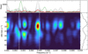 |
Fig. 2 Same as Fig. 1, but for Stokes Q. |
| In the text | |
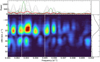 |
Fig. 3 Same as Fig. 1, but for Stokes U. |
| In the text | |
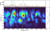 |
Fig. 4 Same as Fig. 1, but for the total linear polarization: |
| In the text | |
|
Fig. 5 Lomb–Scargle periodogram of the 100 photo-center displacement series of Betelgeuse. Each blue line corresponds to a Lomb–Scargle periodogram of one photo-center displacement. The black line is the average of the 100 periodograms. The red dashed lines represent the 400 and 200 d period, respectively. The green line is the window function. The black horizontal line marks the 1σ confidence level. |
| In the text | |
|
Fig. 6 Light curve of Betelgeuse from AAVSO in the V-band. |
| In the text | |
|
Fig. 7 Spectroscopy vs. Photometry periodograms. Upper panel: Lomb–Scargle periodogram of the mean intensity profile presented in Fig. 1 (red line). Middle panel: periodogram of the light curve since 1990 as retrived from the AAVSO database (blue line). Lower panel: periodogram of the light curve (orange line) from AAVSO when the dates correspond to the TBL observations. In every panel, the green line marks the associated window function. The 400 d and the 200 d periods are marked by the black dashed lines. |
| In the text | |
Current usage metrics show cumulative count of Article Views (full-text article views including HTML views, PDF and ePub downloads, according to the available data) and Abstracts Views on Vision4Press platform.
Data correspond to usage on the plateform after 2015. The current usage metrics is available 48-96 hours after online publication and is updated daily on week days.
Initial download of the metrics may take a while.