| Issue |
A&A
Volume 690, October 2024
|
|
|---|---|---|
| Article Number | A214 | |
| Number of page(s) | 8 | |
| Section | Cosmology (including clusters of galaxies) | |
| DOI | https://doi.org/10.1051/0004-6361/202450985 | |
| Published online | 09 October 2024 | |
The energy shear of protohaloes
1
Departamento de Física Fundamental and IUFFyM, Universidad de Salamanca,
Plaza de la Merced s/n,
37008
Salamanca,
Spain
2
Dipartimento di Fisica e Astronomia, Alma Mater Studiorum Università di Bologna,
via Gobetti 93/2,
40129
Bologna,
Italy
3
INAF-Osservatorio di Astrofisica e Scienza dello Spazio di Bologna,
Via Piero Gobetti 93/3,
40129
Bologna,
Italy
4
INFN-Sezione di Bologna,
Viale Berti Pichat 6/2,
40127
Bologna,
Italy
5
Center for Particle Cosmology, University of Pennsylvania,
209 S. 33rd St.,
Philadelphia,
PA
19104,
USA
6
The Abdus Salam International Centre for Theoretical Physics,
Strada Costiera 11,
34151
Trieste,
Italy
★ Corresponding author; mmusso@usal.es; shethrk@upenn.edu
Received:
4
June
2024
Accepted:
10
August
2024
As it collapses to form a halo, the shape of a protohalo patch is deformed by the initial shear field. This deformation is often modeled using the ‘deformation’ tensor, constructed from second derivatives of the gravitational potential, whose trace gives the initial overdensity. However, especially for lower mass protohaloes, this matrix is not always positive definite: one of its eigenvalues has a different sign from the others. We argue that the evolution of a patch is better described by the ‘energy shear’ tensor, which is actually positive definite and plays a direct role in the evolution, and test our analytical result against N-body simulations. We discuss the implications of this positive-definiteness for analytical models of halo abundances, assembly and of the cosmic web.
Key words: cosmology: theory / dark matter / large-scale structure of Universe
© The Authors 2024
 Open Access article, published by EDP Sciences, under the terms of the Creative Commons Attribution License (https://creativecommons.org/licenses/by/4.0), which permits unrestricted use, distribution, and reproduction in any medium, provided the original work is properly cited.
This article is published in open access under the Subscribe to Open model. Subscribe to A&A to support open access publication.
1 Introduction
Understanding how dark matter haloes form and cluster – how their abundance and spatial distribution evolve – potentially unlocks a wealth of information about cosmology and provides the scaffolding on which models of galaxy formation are built. In addition, the intrinsic distribution of halo shapes is a leading systematic for constraining cosmological models with the next generation of galaxy cluster surveys. Thus, the topic of halo formation has been the subject of a significant amount of work.
Numerical simulations have shown that protohalo patches, which evolve into virialised haloes at later times, form from special regions in the initial fluctuation field. Following Bardeen et al. (1986), most models of halo formation associate protohalo patches with peaks in the smoothed overdensity field, which then ‘collapse’ due to gravitational instability. The simplest models assumed the patch and its collapse were both spherically symmetric (Gunn & Gott 1972), with later work exploring ellipsoidal, rather than spherical, collapse (Bond & Myers 1996; Sheth et al. 2001).
These models typically distinguish between the ‘shape’ and the ‘deformation’ or ‘tidal’ tensor of the initial patch. The latter uses the anisotropy of the second spatial derivatives of the potential to infer how the initial shape is deformed. However, to approximate the initial shape, it is usual to use the tensor of second spatial derivatives of the density field. Since the two tensors are correlated, this proxy for the protohalo shape predicts preferential alignment of the shortest axis (corresponding to the steepest descent direction) with the direction of fastest infall (van de Weygaert & Bertschinger 1996): that is, in these models, an initial sphere becomes increasingly non-spherical if the deformation tensor is anistropic. However, if one uses the actual positions of the particles that make up the patch to define the initial inertia tensor, then one finds that the initial shapes are not spherical. Furthermore, they exhibit a strong preferential alignment, with the longest axis of the inertia tensor oriented in the direction of fastest infall (Porciani et al. 2002b; Despali et al. 2013; Ludlow et al. 2014). This alignment has a transparent physical interpretation: it allows particles from further away to reach the halo centre at about the same time as particles that were initially closer, but were collapsing towards the centre more slowly (also see Musso & Sheth 2023). The residual misalignment of the two tensors is instead what gives rise to torques and angular momentum (White 1984; Porciani et al. 2002a; Cadiou et al. 2021).
The word ‘collapse’ suggests that the object shrinks, in comoving coordinates, as it evolves. Stated more carefully, the principal axes of the inertia tensor are expected to shrink as they are squeezed by the velocity flows that define the deformation tensor. Squeezing suggests that the principal axes of the deformation tensor all have the same sign. Indeed, some studies adopted the requirement that all three axes have the same sign as the guiding principle from which to build a model of halo abundances (Lee & Shandarin 1998). However, simulations have shown that this is simply not true for a significant fraction of lower mass protohalo patches (Despali et al. 2013).
Some problems also arise when working with peaks in the matter overdensity field – the trace of the deformation tensor – to identify protohalo centres. There is no guarantee that the density peak coincides with the position onto which the local gravitational flow converges, which is a natural choice to identify the geometric centre of the protohalo patch. Moreover, some of the integrals required to self-consistently define peak statistics diverge. Both disadvantages are overcome if one works with peaks in the energy overdensity field (Musso & Sheth 2021), rather than in the matter overdensity. The main goal of the present work is to show that the energy analogue of the deformation tensor, which we refer to as the ‘energy shear’ tensor, also has an appealing property: all its eigenvalues have the same sign.
We motivate why this sign requirement is expected in Sect. 2, and show tests in simulations in Sect. 3, comparing our results with previous work in Sect. 4. A final section discusses our findings and conclusions.
2 The energy overdensity tensor
In this section, we study the conditions required for the triaxial collapse of protohalo patches of arbitrary shape, before discussing how they relate to analytical models typically based on spherically averaged quantities.
2.1 Evolution of the inertia tensor of protohaloes
The formation of a dark matter halo can be described as the collapse of all three axes of its inertia tensor
 (1)
(1)
where V is a freely evolving volume (in the physical coordinates r) containing the conserved mass M, and rcm denotes its centre of mass. Mass conservation guarantees that time derivatives ‘go through’ the integration sign and the time dependence of ρ(r, t). Thus, the evolution of the inertia tensor of a region comoving with the fluid (the so-called virial equation) is expressed as
 (2)
(2)
where Kij and Uij are the kinetic and potential energy tensors of the body (see e.g. Chandrasekhar 1969; Binney & Tremaine 1987, for the Λ = 0 case). They are defined as
 (3)
(3)
![${U_{ij}} \equiv - \int_V {{{\rm{d}}^3}} r\rho ({\bf{r}},t)\left( {{r_i} - {r_{{\rm{cm}},i}}} \right)\left( {{\nabla _j}\Phi - {{\left[ {{\nabla _j}\Phi } \right]}_{{\rm{cm}},j}}} \right),$](/articles/aa/full_html/2024/10/aa50985-24/aa50985-24-eq4.png) (4)
(4)
where ∇Φ is the gravitational attraction due to matter, so that  , and [∇Φ]cm is the one of the centre of mass.
To describe the evolution of Iij with respect to the background, we split the matter gravitational potential as  , where ϕ is the potential perturbation obeying ∇2ϕ = δm, and
  is the matter density perturbation. We then rewrite Eq. (2) as
 (5)
(5)
where a is the scale factor,  is the Hubble parameter, I ≡ Ikk is the trace of Ii j ,
 (6)
(6)
is the peculiar kinetic energy tensor, and
![${u_{ij}} \equiv {3 \over I}\int_V {{{\rm{d}}^3}} r\rho ({\bf{r}},t)\left( {{r_i} - {r_{{\rm{cm}},i}}} \right)\left( {{\nabla _j}\phi - {{\left[ {{\nabla _j}\phi } \right]}_{{\rm{cm}},j}}} \right),$](/articles/aa/full_html/2024/10/aa50985-24/aa50985-24-eq11.png) (7)
(7)
is the potential energy overdensity tensor, or the ‘energy shear’. The cosmological constant does not appear explicitly in Eq. (5); it only affects the perturbations through its effect on the background evolution of  and H.
Parameterizing the initial value of the comoving inertia tensor as Iij /a2 = (M/5)(AAT)ij, Eq. (5) is solved by
![${{{I_{ij}}} \over {{a^2}}} \simeq {M \over 5}\left[ {{{\left( {A{A^T}} \right)}_{ij}} - D(z)\left( {u_{ij}^{\rm{L}} + u_{ji}^{\rm{L}}} \right){{{\mathop{\rm tr}\nolimits} \left( {A{A^T}} \right)} \over 3}} \right]$](/articles/aa/full_html/2024/10/aa50985-24/aa50985-24-eq13.png) (8)
(8)
at first order in D(z), the growth function of matter density perturbations, since kij is automatically of second order. In this expression,  is the linearized version of uij from Eq. (7) divided by D, and is therefore time independent. For ease of notation, in the following we will drop the superscript L and simply assume that all quantities are evaluated at the lowest order in density perturbations, and rescaled by D(z).
This result can also be obtained directly by writing Eq. (1) in Lagrangian coordinates as
 (9)
(9)
where r − rcm = a(q + Ψ(q, t)) and Ψ is the displacement relative to the centre of mass from the initial comoving coordinate q. At first order in Lagrangian perturbation theory, since Ψ ≃ −D(∇ϕ(q) − [∇ϕ]cm), one gets Eq. (8).
While non-linear dynamics may modify the subsequent evolution, linear theory is sufficient to predict if and when each axis decouples from the Hubble flow and starts recollapsing. Since non-linear corrections, even large ones, manifest themselves at small scales, they will not be able to reverse an ongoing collapse. Hence, the condition for triaxial collapse to happen is that (the symmetric part of) ui j be positive definite: that is, all its eigenvalues have the same sign.
Taking the trace of Eq. (8) returns
![$R_I^2 \equiv {{5I} \over {3M}} \simeq {a^2}{{{\mathop{\rm tr}\nolimits} \left( {A{A^T}} \right)} \over 3}\left[ {1 - 2D(z){ \over 3}} \right],$](/articles/aa/full_html/2024/10/aa50985-24/aa50985-24-eq16.png) (10)
(10)
with є ≡ tr(u), which corresponds (at first order in perturbations) to the result that the collapse of the inertial radius RI is well described by spherical collapse with overdensity є. This is the basis for identifying protohaloes with local maxima of the energy overdensity (Musso & Sheth 2021), since these are minima of the collapse time of RI .
Naively, for a halo to form, one might imagine that all the three axes of the inertia tensor Ii j should collapse at the same time as RI . Equation (8) would then require that
 (11)
(11)
in which case one would have
 (12)
(12)
predicting that the eigenvectors of Ii j and of ui j + uji are to be aligned, and their eigenvalues proportional. This picture is not entirely correct: we know in fact that protohalo boundaries tend to follow equipotential surfaces (Musso & Sheth 2023), which gives an independent prescription for Ii j. It must however be true to some degree, at least for the eigenvectors, since Eq. (8) does show that the anisotropy of ui j favours infall from the direction of strongest compression, with slower infall in the direction of weakest compression.
On the other hand, the mean deformation tensor (sometimes also called shear, or tidal tensor when referring to its traceless part) is defined as
 (13)
(13)
At leading order in perturbations, when  is equal to the gradient of the centre of mass acceleration ∇i[∇jϕ]cm, and its trace, the volume average of ∇2ϕ, equals the mean matter overdensity. We note that although the trace of qi j determines the evolution of the volume V, the tensor qij does not otherwise play a direct role in the evolution of Ii j : what matters is ui j , rather than qij (cf. Eq. (8)).
2.2 Spherical initial volumes
When building models, one often approximates protohaloes as spheres of the same mass. If V is a sphere of radius R centred at x, containing mass  , at leading order in density perturbations its energy overdensity ϵR is
 (14)
(14)
where δL (k) is the linear matter overdensity field normalised to σ8, and W2(kR) ≡ 15j2(kR)/(kR)2 (Musso & Sheth 2021). Similarly, its energy shear is given by
 (15)
(15)
whose trace is given by Eq. (14). Peaks in the energy overdensity field are locations where ∇iєR = 0 and the Hessian
 (16)
(16)
is negative definite.
For a sphere, the mean mass overdensity δR, its deformation tensor qR,ij (whose trace is δR) and its Hessian ∇i∇jδR are obtained replacing W2(kR) in Eqs. (14), (16) and (15) with the standard Top Hat filter W1(kR) ≡ 3j1(kR)/kR. Hence, while the difference between quantities associated with energy rather than mass density is conceptually rather important, in Fourier space the difference simply boils down to using a different, more UV- suppressed smoothing of the overdensity field δ(k) than the usual Top-Hat one.
The distributions of these Gaussian variates are characterised by the spectral moments
 (17)
(17)
where, following Musso & Sheth (2021),
 (18)
(18)
In particular, σ02 and σ22 are the standard deviations of ϵR and ∇2 єR , whereas σ01 and σ21 are those of δR and ∇2δR .
For a homogeneous spherical density perturbation, and only in this case, the two quantities are equal: єR = δR , and the traceless parts of uij and qij are both zero. This is because only the k = 0 mode of δ(k) matters in this case, but both filters tend to 1 as k → 0, hence they make no difference.
2.3 Quantifying the amount of anisotropy
The anisotropic strength of the protohalo environment can be quantified by the magnitude of the traceless shear
 (19)
(19)
We note that the suffix u is to distinguish it from the analogous variable that can be defined from the traceless part of the deformation tensor, which is often called q because it contributes a quadrupolar signature in perturbation theory.
For a random Gaussian matrix, and therefore for random, unconstrained positions in a Gaussian field, this random variate would not be correlated with ϵ (the trace of uij) and would follow a χ2-distribution with five degrees of freedom (Sheth & Tormen 2002). However, it is easy to see that simply requesting the energy shear to be positive definite induces a correlation between the two variables. In fact, since
 (20)
(20)
and the right hand side is positive when all eigenvalues are positive, if uij is positive definite then one has that ϵ > qu. Furthermore, the limit can be saturated only if all three eigenvalues are zero, which never happens in practice.
Some intuitive understanding of this correlation can be obtained by noticing that if ϵ is small, then all eigenvalues are likely to be equally small (since they all have the same sign). Hence, their differences must be small as well. In the following, we look for this correlation in the statistics of protohaloes.
3 Simulation measurements
As the next step, we test our ansatz on the positivity of the eigenvalues of the energy overdensity tensor in the protohaloes of two simulations from the SBARBINE suite (Despali et al. 2016), namely Bice and Flora. Both simulations contain 10243 dark matter particles in a periodic box of side Lbox = 125 h−1 Mpc and Lbox = 2 h−1 Gpc, with initial conditions generated at z = 99. The corresponding particle masses are 1.55 × 10⁸ h−1 M⊙ for Bice and 6.35 × 10¹¹h−1 M⊙ for Flora. The simulations adopt a Planck13 background cosmology: Ωm = 0.307, ΩΛ = 0.693, σ8 = 0.829 and h = 0.677.
Haloes are identified at z = 0 using a Spherical Overdensity halo finder with a density threshold of 319 times the background density, corresponding to the virial overdensity. Our Flora sample contains 5378 haloes, distributed as follows: all the 1378 haloes more massive than 1015h−1 M⊙, 2000 randomly selected haloes with masses between 1014 and 1015h−1 M⊙, and 2000 randomly selected haloes with masses between 4 × 10¹³ and 1014h−1 M⊙. Our Bice sample contains 5000 randomly selected haloes with masses between 1011 and 4 × 10¹³h−1 M⊙. For each halo identified at z = 0, we use ‘protohalo’ to refer to the region occupied by that halo’s particles in the initial conditions.
Since we are interested in initial quantities, we work with the first snapshot of the simulation. We measured each protohalo’s centre of mass position and velocity, qcm and vcm , by averaging over all its particles. We then constructed estimators for its inertia and potential energy overdensity tensor, defined in Eqs. (1) and (7):
 (21)
(21)
 (22)
(22)
where D is the ΛCDM density perturbation growth factor (at the redshift z of the snapshot), f = d In D/d In a, and n runs over the NH protohalo particles. We note that Iij is not divided by NH. To obtain accelerations from velocities we used the Zel’dovich approximation, in which  .
.
For each protohalo we also measured the mean deformation tensor, defined in Eq. (13) as the average over the protohalo particles of the second spatial gradient of the gravitational potential at each position. Since we need to take one more derivative, instead of getting the accelerations from the particle velocities (evaluated at irregular positions), we computed the gradient of the initial displacements that were imposed to create the initial conditions with N-GenIC (Springel et al. 2005), which are computed on the grid. In practice, we selected the grid points occupied by each protohalo, took their initial displacement field Ψ, and estimated the mean deformation tensor Eq. (13) as:
 (23)
(23)
where NG is the number of grid cells contained within the Lagrangian protohalo volume. This means that we also included empty grid cells (i.e. those not occupied by halo particles) that are located inside the Lagrangian volume, because they too contribute to the total potential field that acts on the protohalo. This slightly refines the measurement one obtains if one uses the particle grid points only (see Despali et al. 2013, for more details).
The left panel of Fig. 1 shows the eigenvalues λ1, λ2 and λ3 of  as a function of halo mass. In the range of masses that we sampled, only one out of the 5378 Flora protohaloes had one slightly negative eigenvalue. For Bice protohaloes, which extend to much lower masses, this fraction rises to 0.5% including only haloes more massive than 1012h−1 M⊙, and to nearly 5% for all haloes in the sample. Nevertheless, this is substantially smaller than the fractions shown in Despali et al. (2013) for densitybased statistics (i.e. the eigenvalues of qij) which we also show in the right panel of Fig. 1. This fraction amounts to about 40% of all protohaloes, and nearly half of those between 1011 h−1 M⊙ and 1012h−1 M⊙. Even at masses close to 1014h−1 M⊙ one of the eigenvalues may still be negative. This obvious difference, namely, that the energy shear tensor is positive-definite even when the deformation tensor is not, is the main result of this work.
The left panel of Fig. 2 shows the distributions of the three eigenvalues of  , scaled by σ02 defined in Eq. (17), in the two simulations: filled histograms are for Flora protohaloes more massive than 4 × 10¹⁴h−1 M⊙, while empty ones are for Bice protohaloes more massive than 1011h−1 M⊙. Less massive objects clearly have smaller λi/σ02 . This is not so surprising, since we know that the trace, є = Σi λi, depends on mass (Musso & Sheth 2021). More precisely, whereas the unnormalised ϵ increases at smaller masses, ϵ/σ02 tends to decrease, which explains why all the λi /σ02 tend to be smaller. To remove this dependence, we consider the eigenvalues of the traceless part of
  ,
,
 (24)
(24)
again normalised by σ02. Their distribution is shown in the right panel of Fig. 2 (for the same objects and with the same color coding). Now the histograms of the two simulations (filled and empty) are very similar, showing that these distributions are nearly mass independent.
A detailed analysis of the mutual alignment of the three eigenvectors of the inertia tensor with those of the energy shear is shown in the panels on the left of Fig. 3. This alignment is quite strong, and stronger than the one with the deformation tensor, shown for comparison in the panels on the right. Interestingly, in both cases the alignment is better in Bice (i.e. for smaller halo masses) than in Flora (larger masses).
To get a more concise description of the overlap of the inertia tensor with the energy shear, for each protohalo we computed the matrix cosine
 (25)
(25)
which quantifies with a single number the alignment between the eigenvectors of the two matrices and the similarity of their eigenvalues. We repeated the same measurement for the deformation tensor. A value of the cosine closer to 1 indicates stronger alignment, and is what Eq. (12) would predict exactly. The orange histograms in Fig. 4 show that most measured cosines are greater than 0.9, although the alignment is slightly better for massive haloes (filled histogram). For comparison, the blue histograms show the result of replacing  with the deformation tensor
  : clearly, the inertia tensor is better aligned with the energy shear than with the deformation tensor.
Fig. 5 shows a direct comparison of the eigenvalues  of the inertia tensor and λi of the energy shear, each normalised by their sum (I and ϵ, respectively). Equation (12) would predict that
  for all three i, implying that evolution preserves the protohalo shape, at least at linear order. This is clearly a better approximation for massive haloes (solid histograms), which tend to have ρ2 ∼ 1 but ρ1 tends to exceed, and ρ3 to be less than, unity. Although the ρi = 1 prediction is clearly not verified, it is not that off the mark: for example, we never see ρi ≫ 1. Figure 5 suggests that protohaloes are slightly less elongated than they would have been if ρi = 1, implying that the shear acts to deform the initial shape into a more spherical configuration. Before moving on, we note that, although ρi = 1 has a simple physical interpretation (namely, that evolution preserves the shape), it is not obviously the most natural prediction. We will return to this point in the final discussion section.
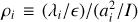
We now consider the shear  , which is expected to play a role in determining the collapse of RI and, hence, the evolution of the shape. The histograms in Fig. 6 show the distribution measured in protohaloes (in Flora and Bice respectively) of the shear strength
  defined in Eq. (19). This distribution is broader than a
  , shown for comparison by the smooth solid curve, which would be expected if the eigenvalue of the energy overdensity tensor were free to take up any sign. Nevertheless, it is still rather mass independent, consistent with the fact that qu is made from traceless eigenvalues, and for these, scaling by σ02 removes most mass dependence (see right-hand panel of Fig. 2).
Finally, a scatter plot of є versus qu (colored by protohalo mass) is displayed in Fig. 7. It shows a strong degree of (approximately linear) correlation between the two variables. This behaviour is also a consequence of all the eigenvalues of uij being positive, as argued in Sect. 2.3.
 |
Fig. 1 Left panel: eigenvalues of the potential energy overdensity tensor uij. Only 5% of protohaloes have one negative eigenvalue; this is our main result. Right panel: eigenvalues of the mean deformation tensor. The lowest eigenvalue is negative in about 40% of protohaloes, and in more than 50% of the lower mass ones, in stark contrast to the left panel. |
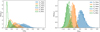 |
Fig. 2 Left panel: distribution of the (normalised) eigenvalues λi of the potential energy overdensity tensor. Filled and open histograms show results for all sampled protohaloes having masses larger than 4 × 10¹⁴h−1 M⊙ (from Flora) and larger than 1011 h−1 M⊙ (from Bice), respectively. Right panel: same, but now for the eigenvalues |

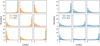 |
Fig. 3 Cosine of the angle θij between the i-th eigenvector of the inertia tensor and the j-th one of the energy shear (left) or of the deformation tensor (right). The alignment with the energy shear is stronger. |
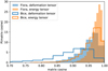 |
Fig. 4 Distribution of the matrix cosine (Eq. (25)) of the inertia tensor Iij with the energy shear tensor uij (orange) or the deformation tensor qij (blue). Filled histograms are for Flora (massive haloes) and empty ones for Bice (smaller masses). |
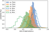 |
Fig. 5 Ratios of the i-th eigenvalue λi of the energy shear Uįj to the i-th eigenvalue |

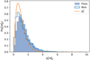 |
Fig. 6 Distribution of |

4 Comparison with previous works
Our analysis bears some qualitative similarity with the results of Bond & Myers (1996), but with two important differences. First, they considered an initially spherical region, in which case AAT in Eq. (8) would be diagonal and reduce to R2δij, where R is the Lagrangian radius of the sphere. While this approximation can be useful and significantly simplifies the calculations, protohaloes are not spherical (or even ellipsoidal), but have rather irregular shapes.
Second, these authors focussed on the deformation tensor qij, rather than on uij. This is correct only under the assumption (which they make) that V is spherical (or at least ellipsoidal) and homogeneous, in which case the two tensors are identical. Under this assumption, there is an exact analytical expression for the potential of the ellipsoid. Working with uij is, on the other hand, completely general (albeit based on a perturbative expansion) and is therefore the correct choice for describing the collapse of the inertia tensor Iij. The downside is that uij has no closed analytical expression in terms of Iij (to be expected, since it also depends on the density profile, except for particular, highly symmetrical cases).
Porciani et al. (2002b), and also later Ludlow et al. (2014), dropped the spherical protohalo assumption, but continued to assume that the deformation tensor provides the natural framework for understanding evolution. In particular, they assumed that protohaloes are ellipsoidal with the longest axis being exactly aligned with the direction of maximum compression of the deformation tensor. While this assumption works well in practice, our analysis here suggests that it has no fundamental physical justification. Rather, its accuracy is more of statistical origin (and is not as good as the one with the energy shear). Furthermore, an exact alignment would not generate angular momentum via gravitational coupling, since the torque induced by the external gravitational field on the protohalo is zero.
On the other hand, as shown by Musso & Sheth (2023), protohaloes are well approximated by equipotential surfaces that deviate from spherical symmetry in response to the local anisotropy of the infall potential. This gives an independent prescription for determining the initial protohalo shape, which then evolves under the action of uij. The symmetric part of uij determines the collapse and deformation, and the antisymmetric one the torque (Musso & Sheth 2023), which can then generate angular momentum as described by Cadiou et al. (2021) (but see also Ebrahimian & Abolhasani 2021).
Despali et al. (2013) studied the eigenvalues of the deformation tensor, and noted that at lower masses (below 1013 h−1 M⊙) it is common for one of them to be negative. In hindsight, this is not surprising since in a generic setup the average of ∇i∇jϕ (that is, qij) describes the gradient of the centre of mass acceleration (see discussion at the end of Sect. 2.1), which is not directly implicated in the collapse dynamics. Rather, as we argue here, triaxial contraction follows from the positivity of the eigenvalues of the energy shear uij, which our measurements in Fig. 1 confirm.
Working with uij has also practical advantages. For a ΛCDM power spectrum the variance of ∇i∇jϵR remains finite, whereas that of ∇i∇jδR diverges. For ϵR it is thus possible to carry out the full calculation of the peak number density from first principles, without having to resort to hand-waving changes of the smoothing filter like in a δR-based approach (Musso & Sheth 2021). However, one might also be interested in other statistics, such as the number density of points with null determinant. These are the so-called critical events (Hanami 2001), where an eigenvalue changes sign, because (for instance) a peak and a saddle point merge and disappear as the smoothing scale R changes. These events are Lagrangian proxies for halo mergers (Cadiou et al. 2020). Computing their number density would require taking one extra derivative, but the variance of the third derivative diverges, this time also for ϵR . On the other hand, if the eigenvalue changing sign is that of uij, the calculation remains well behaved. Defining critical events in terms of the energy tensor, rather than the Hessian, would thus not only come with a stronger connection with dynamics, but also sounder mathematical properties.
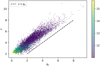 |
Fig. 7 Correlation between the energy overdensity є and the traceless energy shear u of protohaloes. The color coding displays the (logarithm of the) halo mass. The dashed line shows the limiting value (є = qu). |
5 Conclusions
Our measurements strongly support the conclusion that protohalo patches can be identified with regions where the energy overdensity tensor is positive definite. This fact is not a simple statistical correlation, but a dynamical feature that follows directly from the evolution equations of the inertia tensor, which must collapse along three axes. On the other hand, the failure of the deformation tensor defined by the mass overdensity to predict triaxial collapse also has an explanation. While this tensor is directly related to the change of shape of a microscopic volume element, for a macroscopic body its physical interpretation is rather that of the gradient of the centre of mass acceleration: therefore, it is not directly related to the collapse dynamics.
We have thus added another ingredient to the recipe for characterizing protohaloes in terms of energy-related quantities:
the centre of mass of a protohalo is much better identified by a local maximum of the energy overdensity field than of the matter overdensity (Musso & Sheth 2021);
protohalo shapes and boundaries can be described by equipotential surfaces, which further maximise the enclosed energy with respect to spherical configurations (Musso & Sheth 2023);
the energy overdensity tensor (whose eigenvalues must be all positive) does a much better job at predicting both the collapse of the three axes and their initial orientation than the deformation tensor (this work).
More specifically, we have shown that the principal axes of the inertia tensor of protohaloes are very well aligned with the eigenvectors of the energy tensor; the latter identify the main directions of compression of the protohalo region. The longest and shortest protohalo axes tend to align with the directions of maximum and minimum compression, corresponding to the largest and smallest eigenvalue of the energy tensor (for which infall is respectively favoured and disfavoured). Moreover, no collapse should be possible if one eigenvalue is negative. Our measurements strongly support this prediction: less than 5% of protohaloes down to 1011 h−1 M⊙ have one negative eigenvalue (and even then, only slightly negative); none has two negative values.
We also showed that the initial evolution of the protohalo patch is such that it does not quite preserve its initial shape (ρi , 1 in Fig. 5). This is not surprising, as the final shape is usually quite different from the initial one, so ρi ≠ 1 is not a natural or generic prediction. The approach of Musso & Sheth (2023), which provides a prescription for predicting where the boundary of a protohalo lies, allows one to make a more physically motivated prediction for ρi . This is because, once the boundary has been specified, one can estimate both Iij and uij, and, hence, ρi. Working this out explicitly is the subject of ongoing work. Specifying the shape has another important consequence, which we discuss below.
Our findings are important for several reasons. First, they give an effective and unambiguous description of the protohalo environment: protohaloes can be identified with regions having positive definite energy overdensity tensor, as this is what triggers triaxial collapse. Second, while the trace of the tensor (the energy overdensity ϵ) sets the time of collapse and therefore determines the current halo mass, its traceless part (the traceless energy shear) provides a set of variables that can be used to describe assembly bias. It can incorporate effects of the anisotropy of the environment (as done e.g. by Sheth & Tormen 2002; Musso et al. 2018, using the tidal deformation tensor, the analogous quantity for the density), and would appear naturally in symmetry-based bias expansions (Sheth et al. 2013; Lazeyras et al. 2016; Desjacques et al. 2018).
In fact, in our formulation, the energy shear is expected to source the first correction to the collapse time of RI , and, hence, to appear in any analytical expression of a critical threshold for ϵ. Fig. 6 shows that, simply by working with  , the mass-dependence can be nearly scaled-out; this should vastly simplify the development of analytic models of the effects of anisotropies on halo collapse. Typically, such models are built using spherically averaged quantities. This is not ideal since we know that protohaloes are not spherical. Quantifying how this non-sphericity impacts both qu and σ02 , within the context of the minimal energy approach of Musso & Sheth (2023), is the subject of current work.
Furthermore, our analysis also shows (see Fig. 7) that the positivity of the eigenvalues introduces a strong correlation between ϵ and the traceless shear (which would be independent if uij were a generic Gaussian matrix, or equivalently, at random locations in the Gaussian field). This can help to explain the scatter and the trend with mass of the measured values of ϵ in protohaloes (Musso & Sheth 2021), thus enabling the construction of a physically motivated model of the collapse threshold in the energy-based approach. This would provide a natural way for the approach to include assembly bias effects, and is the subject of ongoing work.
There are also a number of practical implications for analytical models of halo aboundance and of the cosmic web. For instance, haloes are typically identified with peaks in the (matter or) energy overdensity field. To distinguish between peaks and other stationary points, one requires that the Hessian of the field be positive definite (Bardeen et al. 1986). However, one can replace this constraint on the Hessian with the same requirement on the energy overdensity tensor. Since the two tensors are correlated, the Hessian would then acquire a mean value proportional to −γui j, where γ denotes the normalised correlation coefficient between −∇2ϵ and ϵ. Thus, it is likely that if uij is positive definite, then so is the negative Hessian, and the point is a peak.
For a more quantitative grasp of the effect, we note that requiring positive definiteness shifts the mean of ϵ from zero to 〈є|+〉 ≈ l.65σ02 (see e.g. Lee & Shandarin 1998). The trace of the Hessian x is commonly used to denote the peak ‘curvature’. If γ denotes the normalised correlation coefficient between x and ϵ, requiring positive definiteness of ϵ shifts the mean of x to 〈є|+〉/σ22 ≈ γ〈є|+〉/σ02 ≈ l.65γ; that is, the trace of the Hessian is likely to be positive, so the Hessian itself is likely to be positive definite, without explicitly requiring it to be so.
Besides the Hessian, which requires two derivatives of the field, some models of the cosmic web make use of third derivatives to identify the disappearance of peaks (or other stationary points) via mergers (Hanami 2001; Cadiou et al. 2020). In a ΛCDM scenario, the energy-based approach is attractive because the statistics of its second derivatives depend on integrals that do not diverge. However, the statistics of its third derivatives still diverge; thus, to estimate abundances of mergers will require using a different (essentially ad hoc) filter. Our results suggest that more principled progress can be made by replacing the Hessian of the energy overdensity field with the energy tensor. This would enable to estimate the relevant statistics (which now have the same degree of convergence in k-space as a gradient) without mathematical ambiguities. In other words, a constraint based on actual collapse dynamics is likely better suited for this task than a merely topological one, and, like for energy peaks, considering a better-motivated physical quantity also solves the mathematical issues in the calculation of the statistics.
The idea of replacing the role of the Hessian with the energy overdensity tensor can be naturally extended to other constituents of the cosmic web (Bond et al. 1996). The signature of the eigenvalues of the energy tensor could be used as the fundamental marker that distinguishes between different cosmic web environments: the four possible different signatures of the potential energy tensor should be used to characterise nodes, filaments, walls and voids. In all these cases, the underlying physical interpretation of the energy tensor, based on predicting the collapse or expansion of the various axes, would be the same. It would be interesting to investigate how well this approach could reproduce properties of the cosmic web that are usually studies with density-based methods, such as its skeleton (Pogosyan et al. 2009) or connectivity (Codis et al. 2018).
A classification of the constituents of the cosmic web based on the dynamical role of the energy shear would connect with the well-established literature on using the signature of the deformation tensor (i.e., the Hessian of the potential rather than of the density) to characterise the cosmic web (e.g. Hahn et al. 2007; Feldbrugge et al. 2023, but also Shen et al. 2006). Our work suggests that using the potential energy tensor instead should be more robust. Perhaps more importantly, as Fig. 1 shows, the signatures of the potential energy and deformation tensors can be different, so the actual cosmic web classifications will differ. Another obvious connection would be with the various works that have tried to predict the emergence of the cosmic web from the formation of caustics in the velocity field (Arnold et al. 1982; Hidding et al. 2014; Neyrinck 2012; Feldbrugge et al. 2018). Unlike these works, which investigate the microscopic properties of the velocity field, the approach based on the energy shear attempts to predict the evolution of macroscopic volumes. It is therefore more suitable to make analytical estimates of the statistics of objects.
Finally, as a practical matter, the measurement of uij in simulations is very straightforward, since it only depends on positions and velocities of protohalo particles. In contrast, measuring qij requires to compute the gradient of the displacement, which must be done at grid points with extra interpolation work.
Acknowledgements
We are grateful to the anonymous referee for an encouraging report. Thanks to Jens Stücker, Corentin Cadiou and Dmitri Pogosyan for helpful discussions, and to the organisers and participants of the 2023 KITP Cosmic Web workshop. Our visit to KITP was supported by the National Science Foundation under PHY-1748958. M.M. and R.K.S. thank the ICTP, Trieste for hospitality when this work was completed. MM acknowledges support from Project PID2021-122938NB-I00 funded by the Spanish “Ministerio de Ciencia e Innovación” and FEDER “A way of making Europe”. G.D. acknowledges the funding by the European Union - NextGenerationEU, in the framework of the HPC project – “National Centre for HPC, Big Data and Quantum Computing” (PNRR - M4C2 - I1.4 - CN00000013 – CUP J33C22001170001).
References
- Arnold, V. I., Shandarin, S. F., & Zeldovich, I. B. 1982, Geophys. Astrophys. Fluid Dyn., 20, 111 [NASA ADS] [CrossRef] [Google Scholar]
- Bardeen, J. M., Bond, J. R., Kaiser, N., & Szalay, A. S. 1986, ApJ, 304, 15 [Google Scholar]
- Binney, J., & Tremaine, S. 1987, Galactic Dynamics (New Jersy, USA: Princeton University Press) [Google Scholar]
- Bond, J. R., & Myers, S. T. 1996, ApJS, 103, 1 [NASA ADS] [CrossRef] [Google Scholar]
- Bond, J. R., Kofman, L., & Pogosyan, D. 1996, Nature, 380, 603 [NASA ADS] [CrossRef] [Google Scholar]
- Cadiou, C., Pichon, C., Codis, S., et al. 2020, MNRAS, 496, 4787 [Google Scholar]
- Cadiou, C., Pontzen, A., Peiris, H. V., & Lucie-Smith, L. 2021, MNRAS, 508, 1189 [NASA ADS] [CrossRef] [Google Scholar]
- Chandrasekhar, S. 1969, Ellipsoidal Figures of Equilibrium (New Haven, CT, USA: Yale University Press) [Google Scholar]
- Codis, S., Pogosyan, D., & Pichon, C. 2018, MNRAS, 479, 973 [Google Scholar]
- Desjacques, V., Jeong, D., & Schmidt, F. 2018, Phys. Rep., 733, 1 [Google Scholar]
- Despali, G., Tormen, G., & Sheth, R. K. 2013, MNRAS, 431, 1143 [NASA ADS] [CrossRef] [Google Scholar]
- Despali, G., Giocoli, C., Angulo, R. E., et al. 2016, MNRAS, 456, 2486 [NASA ADS] [CrossRef] [Google Scholar]
- Ebrahimian, E., & Abolhasani, A. A. 2021, ApJ, 912, 57 [NASA ADS] [CrossRef] [Google Scholar]
- Feldbrugge, J., van de Weygaert, R., Hidding, J., & Feldbrugge, J. 2018, JCAP, 05, 027 [CrossRef] [Google Scholar]
- Feldbrugge, J., Yan, Y., & van de Weygaert, R. 2023, MNRAS, 526, 5031 [NASA ADS] [CrossRef] [Google Scholar]
- Gunn, J. E., & Gott, J. Richard, I. 1972, ApJ, 176, 1 [NASA ADS] [CrossRef] [Google Scholar]
- Hahn, O., Porciani, C., Carollo, C. M., & Dekel, A. 2007, MNRAS, 375, 489 [NASA ADS] [CrossRef] [Google Scholar]
- Hanami, H. 2001, MNRAS, 327, 721 [NASA ADS] [CrossRef] [Google Scholar]
- Hidding, J., Shandarin, S. F., & van de Weygaert, R. 2014, MNRAS, 437, 3442 [Google Scholar]
- Lazeyras, T., Musso, M., & Desjacques, V. 2016, Phys. Rev., D93, 063007 [NASA ADS] [Google Scholar]
- Lee, J., & Shandarin, S. F. 1998, ApJ, 500, 14 [NASA ADS] [CrossRef] [Google Scholar]
- Ludlow, A. D., Borzyszkowski, M., & Porciani, C. 2014, MNRAS, 445, 4110 [NASA ADS] [CrossRef] [Google Scholar]
- Musso, M., & Sheth, R. K. 2021, MNRAS, 508, 3634 [NASA ADS] [CrossRef] [Google Scholar]
- Musso, M., & Sheth, R. K. 2023, Mon. Not. Roy. Astron. Soc., 523, L4 [CrossRef] [Google Scholar]
- Musso, M., Cadiou, C., Pichon, C., et al. 2018, MNRAS, 476, 4877 [Google Scholar]
- Neyrinck, M. C. 2012, MNRAS, 427, 494 [NASA ADS] [CrossRef] [Google Scholar]
- Pogosyan, D., Pichon, C., Gay, C., et al. 2009, MNRAS, 396, 635 [NASA ADS] [CrossRef] [Google Scholar]
- Porciani, C., Dekel, A., & Hoffman, Y. 2002a, MNRAS, 332, 325 [NASA ADS] [CrossRef] [Google Scholar]
- Porciani, C., Dekel, A., & Hoffman, Y. 2002b, MNRAS, 332, 339 [NASA ADS] [CrossRef] [Google Scholar]
- Shen, J., Abel, T., Mo, H., & Sheth, R. K. 2006, ApJ, 645, 783 [NASA ADS] [CrossRef] [Google Scholar]
- Sheth, R. K., & Tormen, G. 2002, MNRAS, 329, 61 [Google Scholar]
- Sheth, R. K., Mo, H., & Tormen, G. 2001, MNRAS, 323, 1 [NASA ADS] [CrossRef] [Google Scholar]
- Sheth, R. K., Chan, K. C., & Scoccimarro, R. 2013, Phys. Rev. D, 87, 083002 [NASA ADS] [CrossRef] [Google Scholar]
- Springel, V., White, S. D. M., Jenkins, A., et al. 2005, Nature, 435, 629 [Google Scholar]
- van de Weygaert, R., & Bertschinger, E. 1996, MNRAS, 281, 84 [NASA ADS] [CrossRef] [Google Scholar]
- White, S. D. M. 1984, ApJ, 286, 38 [NASA ADS] [CrossRef] [Google Scholar]
All Figures
|
Fig. 1 Left panel: eigenvalues of the potential energy overdensity tensor uij. Only 5% of protohaloes have one negative eigenvalue; this is our main result. Right panel: eigenvalues of the mean deformation tensor. The lowest eigenvalue is negative in about 40% of protohaloes, and in more than 50% of the lower mass ones, in stark contrast to the left panel. |
| In the text | |
|
Fig. 2 Left panel: distribution of the (normalised) eigenvalues λi of the potential energy overdensity tensor. Filled and open histograms show results for all sampled protohaloes having masses larger than 4 × 10¹⁴h−1 M⊙ (from Flora) and larger than 1011 h−1 M⊙ (from Bice), respectively. Right panel: same, but now for the eigenvalues |
| In the text | |
|
Fig. 3 Cosine of the angle θij between the i-th eigenvector of the inertia tensor and the j-th one of the energy shear (left) or of the deformation tensor (right). The alignment with the energy shear is stronger. |
| In the text | |
|
Fig. 4 Distribution of the matrix cosine (Eq. (25)) of the inertia tensor Iij with the energy shear tensor uij (orange) or the deformation tensor qij (blue). Filled histograms are for Flora (massive haloes) and empty ones for Bice (smaller masses). |
| In the text | |
|
Fig. 5 Ratios of the i-th eigenvalue λi of the energy shear Uįj to the i-th eigenvalue |
| In the text | |
|
Fig. 6 Distribution of |
| In the text | |
|
Fig. 7 Correlation between the energy overdensity є and the traceless energy shear u of protohaloes. The color coding displays the (logarithm of the) halo mass. The dashed line shows the limiting value (є = qu). |
| In the text | |
Current usage metrics show cumulative count of Article Views (full-text article views including HTML views, PDF and ePub downloads, according to the available data) and Abstracts Views on Vision4Press platform.
Data correspond to usage on the plateform after 2015. The current usage metrics is available 48-96 hours after online publication and is updated daily on week days.
Initial download of the metrics may take a while.