| Issue |
A&A
Volume 690, October 2024
|
|
|---|---|---|
| Article Number | A179 | |
| Number of page(s) | 12 | |
| Section | Galactic structure, stellar clusters and populations | |
| DOI | https://doi.org/10.1051/0004-6361/202450954 | |
| Published online | 08 October 2024 | |
Inference of black-hole mass fraction in Galactic globular clusters
A multi-dimensional approach to break the initial-condition degeneracies
1
Department of Physics and Astronomy “Augusto Righi”, University of Bologna,
via Gobetti 93/2,
40129
Bologna,
Italy
2
INAF – Astrophysics and Space Science Observatory of Bologna,
via Gobetti 93/3,
40129
Bologna,
Italy
3
Department of Astronomy, Indiana University,
Swain West, 727 E. 3rd Street,
Bloomington,
IN
47405,
USA
★ Corresponding author; e-mail: This email address is being protected from spambots. You need JavaScript enabled to view it.
Received:
31
May
2024
Accepted:
19
August
2024
Abstract
Context. Globular clusters (GCs) are suggested to host many stellar-mass black holes (BHs) at their centers, thus resulting in ideal testbeds for BH formation and retention theories. BHs are expected to play a major role in GC structural and dynamical evolution and their study has attracted a lot of attention. In recent years, several works attempted to constrain the BH mass fraction in GCs typically by comparing a single observable (for example, mass segregation proxies) with scaling relations obtained from numerical simulations.
Aims. We aim to uncover the possible intrinsic degeneracies in determining the BH mass fraction from single dynamical parameters and identify the possible parameter combinations that are able to break these degeneracies.
Methods. We used a set of 101 Monte Carlo simulations sampling a large grid of initial conditions. In particular, we explored the impact of different BH natal kick prescriptions on widely adopted scaling relations. We then compared the results of our simulations with observations obtained using state-of-the-art HST photometric and astrometric catalogs for a sample of 30 Galactic GCs.
Results. We find that using a single observable to infer the present-day BH mass fraction in GCs is degenerate, as similar values could be attained by simulations including different BH mass fractions. We argue that the combination of mass-segregation indicators with GC velocity dispersion ratios could help us to break this degeneracy efficiently. We show that such a combination of parameters can be derived with currently available data. However, the limited sample of stars with accurate kinematic measures and its impact on the overall errors do not allow us to discern fully different scenarios yet.
Key words: black hole physics / methods: numerical / stars: black holes / stars: kinematics and dynamics / globular clusters: general
© The Authors 2024
 Open Access article, published by EDP Sciences, under the terms of the Creative Commons Attribution License (https://creativecommons.org/licenses/by/4.0), which permits unrestricted use, distribution, and reproduction in any medium, provided the original work is properly cited.
This article is published in open access under the Subscribe to Open model. This email address is being protected from spambots. You need JavaScript enabled to view it. to support open access publication.
1 Introduction
Massive stellar clusters are ideal cosmic laboratories of multi-body dynamics (Heggie & Hut 2003) and gravitational wave astrophysics (Rodriguez et al. 2015; Hong et al. 2018). Due to asymmetric supernova explosion, BHs are expected to experience natal kicks (Janka 2013; Mandel 2016): if the kick amplitude is larger than the local escape speed, the BH is ejected. The increasing number of detections of stellar mass BHs in Galactic GCs (Maccarone et al. 2007; Strader et al. 2012; Chomiuk et al. 2013; Miller-Jones et al. 2015; Giesers et al. 2018, see also Gaia Collaboration 2024; Balbinot et al. 2024 for the recent detection of a 33 M⊙ BH in the ED 2 stellar stream) has thus triggered an extensive effort into the study of the long-term retention of BHs in massive clusters. These studies have shown that a sizeable population of BHs could be retained at the center of GCs for timescales longer than the Hubble time (Morscher et al. 2013; Sippel & Hurley 2013; Heggie & Giersz 2014; Arca Sedda et al. 2018; Askar et al. 2018). Also, following the recent discoveries of BH-star binaries by Gaia (Tanikawa et al. 2023; Chakrabarti et al. 2023; El-Badry et al. 2023a,b; Gaia Collaboration 2024) young star clusters were investigated as possible BH formation grounds (Rastello et al. 2023; Tanikawa et al. 2024a,b; Di Carlo et al. 2024). Within this context, BH retention in lower-mass star clusters would place strong constraints on BH natal kicks (see e.g., Torniamenti et al. 2023).
Several works addressed the role and impact of a population of BHs in the long-term dynamical evolution of a stellar system. They showed that the presence of BHs, specifically the heating from dynamically formed binary BHs, can significantly delay the mass segregation of visible stars and the core collapse of GCs (see e.g., Mackey et al. 2007, 2008; Breen & Heggie 2013; Morscher et al. 2015; Alessandrini et al. 2016; Peuten et al. 2016; Weatherford et al. 2018).
However, the BH retention in GCs and the distribution of kick velocities after their formation are still matters of investigation (Belczynski et al. 2002; Repetto et al. 2012; Janka 2013; Mandel 2016; Repetto et al. 2017; Giacobbo & Mapelli 2020; Andrews & Kalogera 2022). The search for stellar-mass BHs in Galactic GCs, therefore, opens up a window on many fundamental and timely science cases, including the constraint of the early BH retention and natal kicks, the study of stellar dynamical interactions, up to the BH-BH merging in dense stellar systems as a source of gravitational wave emission (Moody & Sigurdsson 2009; Banerjee et al. 2010; Rodriguez et al. 2015, 2016b,a, 2018; Antonini & Rasio 2016; Hurley et al. 2016; Askar et al. 2017; Fragione & Kocsis 2018; Hong et al. 2018; Samsing & D’Orazio 2018; Samsing et al. 2018; Zevin et al. 2019, Arca Sedda et al. 2023, 2024a,b; Marín Pina et al. 2024; El-Badry 2024).
Recently, many studies addressed the inference of the total mass in stellar mass BHs harbored by GCs (Askar et al. 2018; Zocchi et al. 2019; Askar et al. 2019; Weatherford et al. 2020; Dickson et al. 2024). In particular, Askar et al. (2018) explored several correlations (obtained from Monte Carlo simulations, see Arca Sedda et al. 2018) to infer the properties of the BH subsystem, if present, using as observational anchor the luminosity density within the half-mass radius. The authors shortlisted 29 GCs that could potentially harbor a significant number (up to a few hundred) of BHs. Weatherford et al. (2020) used a theoretical correlation between the fraction of BHs and the degree of mass segregation (Weatherford et al. 2018) to infer the present-day BH population and their total mass in 50 Galactic GCs. Finally, Dickson et al. (2024) performed multi-mass modeling of several cluster observables (i.e., velocity dispersion profiles along the proper motion (PM) and line-of-sight (LOS) directions, number density profile, and mass function measurements) for 34 GCs, thereby being able to constrain the total dynamical mass in dark remnants at the cluster centers. Interestingly, they found typically lower BH mass fractions compared to Askar et al. (2018), and Weatherford et al. (2020, see e.g. Fig. 3 in Dickson et al. 2024).
As discussed by Askar et al. (2018, see their Sect. 2.6), the inference of the mass in BHs using a single observable can be strongly biased and dependent on the specific assumptions adopted in the analysis. In this work, we thus address the degeneracies in the inference of present-day BH population in GCs, possibly arising from multiple assumptions about the underlying physical processes that are still poorly constrained observationally. The purpose of this work is therefore 1) to point out that some observable structural quantities used in the literature to infer the mass fraction in BHs are consistent both with systems with a significant mass fraction in BHs and systems with no (or a negligible fraction of) BHs; 2) to possibly identify the combination of dynamical parameters that allows unambiguous identification of the presence of a significant population of BHs.
The paper is organized as follows: in Sect. 2 we present the simulation survey and its set of initial conditions, and in Sect. 3 we discuss the parameters investigated and the implications for BH mass fraction-inference in real GCs. In Sect. 4 we describe a detailed comparison between the observations and our set of simulations, trying to disentangle different scenarios. In Sect. 5 we summarize the results and conclude.
2 Methods and initial conditions
In this work, we use a set of 101 Monte Carlo simulations (Hénon 1971a,b) performed with the MOCCA1 code (Giersz et al. 2013; Hypki & Giersz 2013). The MOCCA code follows the evolution of star clusters including the effects of two-body relaxation, single and binary stellar evolution (modeled with the SSE and BSE prescriptions; Hurley et al. 2000, 2002), close stellar interactions (which were integrated by using the FEWBODY code Fregeau et al. 2004), and a spatial cut-off modeling the effect of the tidal truncation due to the host galaxy.
The set of simulations analyzed in this work was fully presented in Bhat et al. (2024) in the context of defining novel structural parameters to determine the stage reached by GCs in their evolution toward the core-collapse and post-core-collapse phases. Here we briefly summarize the initial conditions adopted and refer to that paper for further details. Each simulated cluster starts with an equilibrium configuration defined by a King (1966) distribution function, assuming a central dimensionless potential of W0 = 5 or 7. The truncation radii of our models are equal to the tidal radii of clusters moving on circular orbits in a logarithmic potential for the Galaxy at galactocentric distances of 2, 4, and 6 kpc. A filling factor (defined as the ratio between the three-dimensional half-mass, rhm, and the tidal, rt, radii) of 0.025, 0.050 or 0.1 was adopted. The number of particles, Np (defined as the sum of the number of single stars and binaries), varies between 500k, 750k, and one million with a 10% primordial binary fraction. The initial distribution of binary properties was set following the eigenevolution procedure described in Kroupa (1995) and Kroupa et al. (2013). Finally, for each set of these initial conditions, two simulations were performed assuming a different prescription for the BH natal kicks: either a Maxwellian distribution with a dispersion of 265 km s−1(i.e., the same as neutron stars, NSs, Hobbs et al. 2005), or a reduced kick velocity based on the fallback prescription by Belczynski et al. (2002). We adopted a Kroupa (2001) stellar initial mass function between 0.1 and 100 M⊙ and a metallicity Z = 10−3. Finally, we did not include 7 simulations in which an intermediate-mass black hole was formed. Studying the impact of intermediate-mass black hole formation on observable cluster properties is beyond the scope of this work, and will be the subject of future studies.
3 Results
In this section, we present the analysis and the properties at 13 Gyr of the simulations in the survey. Firstly, for each simulation, we computed the total stellar mass (MGC) and the BH mass fraction (defined as MBh/Mgc, with MBH being the total mass in BHs). We then explored the impact of long-lived BH subsystems on the evolution of star clusters by computing several quantities, some of which were previously used to infer the presence of massive BH populations in Galactic GCs (see e.g., Mackey et al. 2008; Bianchini et al. 2016; Askar et al. 2018; Weatherford et al. 2020): the mass-segregation parameter (Δ), the average luminosity density, (![Mathematical equation: $\[L_{\mathrm{V}} / R_{\mathrm{hl}}^2\]$](/articles/aa/full_html/2024/10/aa50954-24/aa50954-24-eq1.png) , with Rhl the half-light radius and LV the total V luminosity within Rhl), the concentration ratio (Rc/Rhl with Rc being the core radius), the dynamical age (nh), and the inverse of the equipartition mass (μ) estimated within 0.1Rhl.
, with Rhl the half-light radius and LV the total V luminosity within Rhl), the concentration ratio (Rc/Rhl with Rc being the core radius), the dynamical age (nh), and the inverse of the equipartition mass (μ) estimated within 0.1Rhl.
The parameter Δ was defined as
![Mathematical equation: $\[\Delta=\int_0^1 \mathrm{nCRD}_{\mathrm{pop} 1}(x)-\mathrm{nCRD}_{\mathrm{pop} 2}(x) ~d x,\]$](/articles/aa/full_html/2024/10/aa50954-24/aa50954-24-eq2.png) (1)
(1)
where nCRD is the normalized cumulative radial distribution computed for a more massive (labeled as pop1) and a lower-mass (labeled as pop2) population. The integral is computed between the cluster center and a limiting distance Rlim = 2Rhl with x corresponding to the projected distance of each star from the center, normalized to Rlim. Similar parameters proved powerful tools in studying the properties and dynamical evolution of GCs (see e.g., Alessandrini et al. 2016; Lanzoni et al. 2016; Peuten et al. 2016; Ferraro et al. 2018, 2019, 2023a,b; Raso et al. 2017; Dalessandro et al. 2019), and were already used in previous studies to investigate the role of BH subpopulations within GCs (see e.g., Weatherford et al. 2018). We exploited almost the full stellar mass range available at 13 Gyr to maximize the mass-segregation signal: for the more massive population, we selected stars within [mto − 0.025; mto] M⊙ (with mto = 0.8155 M⊙ being the main-sequence turn-off mass at 13 Gyr for a simple stellar population with Z = 10−3), whereas for pop2 we selected stars in the mass range [0.1; 0.125] M⊙. According to the definition in Eq. (1), Δ is a dimensionless parameter that traces the relative spatial concentration of massive stars compared to lower-mass ones through their nCRDs: the larger the value, the more massive stars are spatially segregated compared to the lower-mass ones.
The proxy for the dynamical age, nh, was defined as the ratio between the cluster physical age and the half-mass relaxation time (trh; Spitzer 1987) calculated at that physical age; following Spitzer (1987):
![Mathematical equation: $\[t_{\mathrm{rh}}=0.138 \frac{M_{\mathrm{GC}}^{1 / 2} r_{\mathrm{hm}}^{3 / 2}}{\langle m\rangle ~G^{1 / 2} ~\ln \Lambda},\]$](/articles/aa/full_html/2024/10/aa50954-24/aa50954-24-eq3.png) (2)
(2)
with G the gravitational constant, ⟨m⟩ the mean star mass, and Λ the Coulomb logarithm coefficient. We used Λ = 0.02 Np, which accounts for the effects of a mass spectrum (Giersz & Heggie 1996).
To compute Rc, we fitted an analytical, multi-power law model to the surface brightness profile in the V band obtained using stars with V < Vto + 2, with VTO being the turn-off magnitude. For each simulation, VTO was estimated by dividing stars into magnitude bins (between V = 17–23 mag, 0.1 mag wide) and selecting the bin with the bluest V − I color. Finally, the core radius was obtained as the radius at which the surface brightness is half the central one. The half-light radius (Rhl) was defined as the radius enclosing half of the total projected light in the V band and computed directly from the simulation.
Finally, we computed the μ(< 0.1Rhl) parameter as presented in Aros & Vesperini (2023). This quantity represents the inverse of the equipartition mass (Bianchini et al. 2016) with the advantage of providing a simpler description of the stellar-mass-dependence of the velocity dispersion (see Aros & Vesperini 2023, for further details).
In Fig. 1, we present all the possible combinations of the aforementioned parameters computed for each simulation. In particular, the bottom row in Fig. 1 shows the BH mass fraction as a function of different properties: the presence of a BH subsystem inhabiting the cluster central regions prevents the core collapse of visible stars thereby delaying the evolution of their structural properties (Mackey et al. 2007, 2008; Breen & Heggie 2013; Morscher et al. 2015). This is in turn reflected in the Rc/Rhl ratio (which increases for higher BH mass fractions, see e.g., Kremer et al. 2020), and the luminosity density (which decreases for increasing BH mass fractions, see the discussion in Arca Sedda et al. 2018).
In Fig. 2, we focus on the BH mass fraction as a function of Δ. When simulations with the fallback prescription are considered, it is possible to observe a nice correlation between the BH mass fraction and Δ, as expected based on the well-established role of binary BHs in halting the mass segregation of massive visible stars (Breen & Heggie 2013). A similar trend was also recovered by Weatherford et al. (2018). However, Fig. 2 also shows that clusters can exhibit little mass segregation (i.e., low values of Δ) without a sizeable population of BHs or even with no BHs at all. These systems have long initial relaxation times and BHs were ejected right after formation due to large natal kicks (for these simulations the fallback off prescription was adopted). Hence, while mass segregation can provide us with valuable information, the role of different initial conditions and physical assumptions should be carefully considered (see also, for instance, the discussion in Sect. 2.6 of Askar et al. 2018). Also, a similar behavior is observed in all the quantities presented in Fig. 1. The fact that clusters with very different BH mass fractions might exhibit similar properties (in terms of mass segregation, concentration ratio, and luminosity density see Fig. 1) highlights the possible problems in inferring the BH mass fraction in real GCs using a single observable. Therefore, multiple physical properties should be jointly used to constrain the presence of BHs within GCs.
In this respect, we introduce a new observable parameter which in synergy with Δ turns out to be particularly useful in discriminating between BH retention and dynamical evolution. This is defined as σμ (< 0.2Rhl)/σμ(Rhl), which is the ratio between the 1D velocity dispersion2 computed within 0.2Rhl and at Rhl3. This parameter quantifies the steepness of the velocity dispersion profile, which directly reflects the radial variation of the gravitational potential.
In Fig. 3, we show the Δ-σμ (< 0.2Rhl)/σμ(Rhl) plot. Low mass segregation levels (roughly Δ < 0.15) can be explained either by the presence of a massive BH subsystem (darker points in Fig. 3) or due to the system being dynamically younger, without requiring high BH mass fractions (lighter points in Fig. 3, but see also Fig. 1). However, these two classes depart in σμ (< 0.2Rhl)/σμ(Rhl): the presence of a massive BH subsystem deepens the potential well in the central regions, increasing the velocity dispersion ratio. On the other hand, dynamically young systems without many BHs exhibit lower values.
Velocity dispersion ratios on the order of 1.15 are attained by systems with low BH mass fractions only if they are dynamically evolved (i.e., roughly Δ > 0.2), effectively breaking the degeneracy between dynamically young GCs without large BH mass fractions and systems hosting a massive BH population which slowed down their dynamical aging.
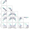 |
Fig. 1 Simulation properties at 13 Gyr, each point representing a different simulation. Moving downwards on the y-axis: luminosity density (in units of L⊙ per2), core to half-light radius ratio (Rc/Rhl), dynamical age (nh), inverse of the equipartition mass, μ(< 0.1Rhl), BH mass fraction (Mbh/MGC), and mass segregation parameter Δ. Simulations are color-coded according to the number of BHs (NBH) at 13 Gyr. A value of log NBH = −0.5 was assigned to those with no BHs. Similarly, simulations that do not retain any BH at 13 Gyr are shown at MBH/MGC = 5 × 10⁻⁶ on the bottom row for visualization purposes only. |
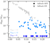 |
Fig. 2 BH mass fraction as a function of Δ. Colors depict the number of BHs in the simulation at 13 Gyr, while different symbols show the adopted fallback prescription in the initial conditions. Simulations without BHs at 13 Gyr are shown at MBH/MGC = 5 × 10⁻⁶. To account for fluctuations in the estimates arising due to the discrete nature of the simulations, we performed 500 different projections along the LOS, and for each of them, we measured Δ. The values shown are the median ones. Errors obtained computing the 16% and 84% percentiles of the distribution are also shown although barely visible. |
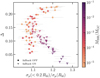 |
Fig. 3 Mass segregation parameter as a function of the velocity dispersion ratio. Symbols show whether the simulation had (diamond) or had not (upside-down triangle) the fallback prescription for BH formation. Different colors depict the BH mass fraction (see the color bar on the side) Finally, error bars were obtained from multiple projections along the LOS. |
4 Observations
In this section, we present the observational analyses carried out for a sample of Galactic GCs to compare their structural and kinematical properties with those from simulations.
4.1 Properties of Galactic GCs
We selected Galactic GCs with both photometric data from Sarajedini et al. (2007) and individual-stars PMs by Libralato et al. (2022)4, covering at least the central 0.7Rhl. Such a selection included GCs proposed as promising candidates for hosting high BH mass fractions (including NGC 5053, NGC 6101, and NGC 6362, see Askar et al. 2018; Weatherford et al. 2020) while allowing to investigate a sufficiently large radial range. A large radial range enables better characterization of the system properties, such as mass segregation and the velocity dispersion profile. Finally, we empirically found that selecting stars down to three magnitudes below VTO was the best compromise between keeping the mass gap between pop1 and pop2 as large as possible and ensuring photometric completeness of at least 0.5 over the whole radial range for a sizable fraction of GCs. In Sect. 4.2, we present the calculation of the photometric completeness and we discuss those cases for which the incompleteness was too severe and the calculation of Δ-like quantities is not feasible with the dataset adopted in this work. Out of the 57 clusters in common between Sarajedini et al. (2007) and Libralato et al. (2022), 30 met all the aforementioned criteria. For cluster ages, masses, and characteristic radii, we used the catalog provided by Baumgardt et al. (2020, but see also Vasiliev & Baumgardt 2021; Baumgardt & Vasiliev 2021)5.
To estimate σμ (< 0.2Rhl)/σμ(Rhl), we used the recent astrometric catalog by Libralato et al. (2022). The catalog consists of PMs and multi-epoch photometry for stars in about the central 100“ of 56 Galactic GCs. We applied the same quality selections presented in Sect. 4 of Libralato et al. (2022) retaining stars with V < VTO + 1.25 (as done for the simulations). Adopting the same spatial selections (Sect. 3), and using Rhl from the catalog by Baumgardt et al. (2020, 4th version), we computed the 1D velocity dispersion accounting for errors on the n individual stars. In particular, we assumed the likelihood function (Pryor & Meylan 1993)
![Mathematical equation: $\[\begin{aligned}\ln \mathcal{L}= & \sum_{i=1}^n-\frac{1}{2}\left(\frac{\left(v_{i, \mathrm{R}}-\left\langle v_{\mathrm{R}}\right\rangle\right)^2}{\sigma_{\mathrm{R}}^2+\delta v_{i, \mathrm{R}}^2}+\ln \left(\sigma_{\mathrm{R}}^2+\delta v_{i, \mathrm{R}}^2\right)\right) \\& +-\frac{1}{2}\left(\frac{\left(v_{i, \mathrm{~T}}-\left\langle v_{\mathrm{T}}\right\rangle\right)^2}{\sigma_{\mathrm{T}}^2+\delta v_{i, \mathrm{~T}}^2}+\ln \left(\sigma_{\mathrm{T}}^2+\delta v_{i, \mathrm{~T}}^2\right)\right),\end{aligned}\]$](/articles/aa/full_html/2024/10/aa50954-24/aa50954-24-eq4.png) (3)
(3)
with υi,R, υi,T being the radial and tangential velocity components for the i-th star, respectively. Each component had its error, namely δυi,R, δυi,T. All the values were computed in mas/yr, independent of any assumption on the cluster distance. Finally, the mean velocities ⟨υR⟩ and ⟨υT⟩, the velocity dispersion components σR and σT, and the 1D velocity dispersion (σμ, see Sect. 3) were computed through a Markov chain Monte Carlo (MCMC) exploration of the parameter space. In particular, we used the emcee package6 (Foreman-Mackey et al. 2013), which provides a Python implementation of the affine-invariant MCMC sampler, enabling us to sample the posterior distribution. The same analysis was carried out for stars within 0.2Rhl and around Rhl, and the 1D velocity dispersion ratio was computed. For clusters with field of view (FoV) coverage smaller than Rhl, we opted for a hybrid approach. We estimated the inner 1D velocity dispersion using individual stars (see Eq. (3)) whereas we relied on dynamical modeling for the outer one. Using a single-mass, King model (King 1966, constructed via the LIMEPY7 Python library developed by Gieles & Zocchi 2015) we fitted both the density (de Boer et al. 2019) and the 1D velocity dispersion (obtained by merging HST data from Libralato et al. 2022, and Gaia DR3 data, Vasiliev & Baumgardt 2021) profiles. The former allowed us to constrain the structural parameters (such as W0, and rhm), while the latter constrained the total cluster mass. We discuss the fitting procedure and present the results in Appendix A.
To quantify mass segregation, we defined the parameter Δobs(< Rlim): similarly to Eq. (1), Δobs(< Rlim) quantifies the degree of segregation via the area between the nCRDs of a bright (BP) and faint (FP) population computed within a given distance, Rlim, from the center. We computed Δobs(< Rlim) using the photometric catalog provided by Sarajedini et al. (2007).
A critical step in this regard was a proper assessment of the photometric incompleteness of the catalogs. Due to crowding, incompleteness mainly affects faint stars, preferentially in the center. Given that Δobs(< Rlim) traces the mass segregation using the relative spatial distributions, incomplete catalogs bias the results in a non-trivial manner, possibly inflating the mass-segregation signal. We therefore estimated the completeness (c) for every star, accounting for its projected distance from the center and magnitude. Finally, each star contributed to the nCRD with a factor 1/c.
4.2 Accounting for incompleteness in evaluating Δobs(< Rlim)
In this Section, we present the details of the photometric completeness calculation, carried out for all the clusters in the sample. In particular, we used the photometric catalog by Sarajedini et al. (2007), and the artificial-star test catalog by Anderson et al. (2008) provided for each cluster. The latter catalog consists of 105 artificial stars, distributed uniformly within the core radius and with a density ∝R−1 outside, with a flat luminosity function in the F606W filter and with colors along the cluster fiducial line (see Anderson et al. 2008, for further details).
To estimate the completeness we adopted the following procedure:
we determined quality selection criteria exploiting the QFIT parameter in both V and I bands as a function of magnitude. Stars with a QFIT higher than the 90th percentile of the distribution at the star magnitude were not considered in the subsequent analyses;
using stars with good photometry, we determined membership selection criteria in the color-magnitude diagram (V versus V − I). Dividing the stars in magnitude bins (0.5 magnitudes wide), we found the 10th and 90th percentiles of the color distribution. Stars outside this range were not included, as probably field interlopers;
we applied these selections to the observed and photometrically-calibrated artificial-star catalogs8. In this step, particular care was paid to keeping artificial stars without an output magnitude, which are those input stars not recovered by the data reduction pipeline;
for each observed star we selected artificial stars within a radial shell centered around the star position. The shell width was iteratively widened until at least 1000 artificial stars were selected. We then constructed the completeness curve as a function of the magnitude. For each magnitude bin, the completeness was directly computed as the ratio between the number of recovered and input artificial stars. We considered a star as recovered if the output and input V magnitudes were compatible with a tolerance of 0.75 magnitudes, due to photometric blends (as suggested by Anderson et al. 2008). The final completeness value assigned to each star was obtained by interpolating this curve and evaluating it at the star magnitude.
We defined the BP as stars with V magnitude [Vto; Vto + 1], whereas FP stars have magnitudes in the range [Vto + 2; VTO + 3]. The limit of V < VTO + 3 ensured that c > 0.5 over the whole FoV while keeping the mass gap between BP and FP stars as large as possible (see also discussion in Sect. 4.1). Lower completeness estimates are indeed more uncertain as the completeness relative error roughly scales as the inverse of the square root of the number of recovered stars. Therefore, retaining stars with very low completeness makes the nCRD more uncertain. Also, evaluating the impact of pushing to very low completeness regimes is not straightforward, as one might over- or underestimate the nCRD due to significant statistical fluctuations in the completeness estimate.
In Fig. 4, we show the completeness properties of FP stars in NGC 6584: as expected, the c decreases toward the center and for fainter magnitudes. However, the FP stars in this cluster are characterized by completeness levels ≳75% at all distances.
In Fig. 5, we show the 2D radial distribution (left panel) and completeness variation curves (right panel) for NGC 7089 as a prototypical case of a cluster excluded from our analysis. While this GC fulfills the radial coverage requirements (Sect. 4.1), its FP is characterized by a strong incompleteness in the innermost regions. In fact, for this sub-sample of stars c decreases rapidly towards the center, dropping well below the critical threshold of 0.5 around Rhl, and almost no stars are found within <0.5 Rhl. Such severe incompleteness makes the calculation of Δobs(< Rlim) practically unfeasible. We note that a few similar cases (for example NGC 2808, and NGC 6093) were included in the analysis by Weatherford et al. (2020) with a possible significant impact on the derived values of Δ for these systems.
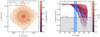 |
Fig. 4 Photometric completeness for NGC 6584. Left panel: two-dimensional map of sources in the magnitude range [VTO + 2; VTO + 3], with VTO being the turn-off magnitude. Each star is color-coded according to the completeness in the V band. Right panel: V-magnitude dependence of the photometric completeness. Stars are color-coded according to their projected distance from the center normalized to Rhl. The gray area marks c < 0.5 whereas the blue region shows the [VTO + 2; Vto + 3] magnitude range. |
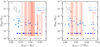 |
Fig. 6 BH mass fraction as a function of Δobs(< Rhl) (left panel) and Δobs(< 0.7Rhl) (right panel). Points show the simulation properties recomputed according to the magnitude and spatial selections adopted for the observations (see Sect. 4.1), whereas the vertical red lines show values obtained for the Galactic GCs studied in this work (along with errors as shaded areas). Simulations without BHs at 13 Gyr are shown at MBH/MGC = 5 × 10⁻⁶. |
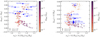 |
Fig. 7 Δobs(< Rhl) (left panel) and Δobs(< 0.7Rhl) (right panel) as a function of the velocity dispersion ratio. Values from the simulations were recomputed according to the magnitude and spatial selections adopted for the observations (see Sect. 4.1). Simulations are color-coded according to the BH mass fraction (see the color bar). Error bars were computed from multiple LOS projections. Finally, in blue we show the values (along with error bars) obtained for Galactic GCs (see Sect. 4 for details). The observations shown in this plot are reported in Tables B.1 and B.2. |
4.3 Comparison with simulations
Here, we compare the results obtained from the simulations (Sect. 3) and the state-of-the-art data presented in Sect. 4.1.
Fig. 6 shows the BH mass fraction as a function of Δobs(< Rlim) for Rlim = Rhl (left panel) and Rlim = 0.7Rhl (right panel). Values from both simulations and observations were computed according to the definition in Sect. 4.1, adopting Rlim = Rhl (0.7Rhl for those GCs with smaller FoV coverage), and using BP and FP stars to compute Δ. The simulations cover a similar range of Δobs(< Rlim) as the observations. In addition, each value of Δobs(< Rlim) could be reproduced by either simulation with high or low BH mass fractions. This further highlights the degeneracies and strengthens the need for a multi-dimensional approach.
Fig. 7 shows Δobs(< Rlim)-vs-σμ (< 0.2Rhl)/σμ(Rhl). Simulations are color-coded according to the BH mass fraction, with different symbols depicting whether the fallback prescription was adopted for the BH natal kicks. Finally, blue points show the values obtained for Galactic GCs (see Sect. 4.1). In particular, we show only those clusters for which at least 100 stars with kinematics were available in the radial ranges considered. Such a threshold ensures that the errors on σμ (< 0.2Rhl)/σμ(Rhl) are small enough for a meaningful comparison with the simulations. Nonetheless, in Table B.1 we provide the values of Δobs(< Rlim) for all the clusters, and σμ(< 0.2Rhl)/σμ(Rhl) (and relative errors) for the clusters shown in Fig. 7.
The left panels of Figs. 6, and 7 show GCs for which the data coverage was ≥ Rhl. For these clusters the Δobs(< Rhl) and σμ(< 0.2Rhl)/σμ(Rhl) values are in reasonable agreement with numerical-simulation predictions except for a few cases that show discrepant values of Δobs(< Rhl). Also, they typically show Δobs(< Rhl) ≳ 0.03 (see also Table B.1). The mass segregation and the kinematic properties of these clusters could be thus reproduced either by systems in which BHs were ejected right after formation (due to high natal kicks) or that lose their BHs due to dynamical interactions in the center. In either case, the present-day BH mass fraction is likely low (similarly to what was found by Weatherford et al. 2020; Dickson et al. 2024).
As discussed in Sect. 4.1, we also considered GCs with a FoV coverage smaller than Rhl. Within this sample, a few notable clusters were indeed suggested to host massive BH populations at their center (e.g., NGC 5053, NGC 6101, and NGC 6362, see Askar et al. 2018; Weatherford et al. 2020). The right panel of Fig. 6 shows the Δobs(< 0.7Rhl) values obtained for these GCs. As expected from previous works (Dalessandro et al. 2015; Peuten et al. 2016; Weatherford et al. 2020) some of these clusters exhibit little mass segregation. This feature could be interpreted as either the result of the BH burning phase (Kremer et al. 2020) or slow dynamical evolution, as already discussed in Sect. 3.
In the right panel of Fig. 7, we delve more into the kinematic properties of these clusters using σμ (< 0.2Rhl)/σμ(Rhl) introduced in this work: focussing on clusters with little mass segregation (roughly Δobs(< 0.7Rhl) < 0.02, see the right panel of Fig. 7) we notice that while there might be hints of higher values of σμ(< 0.2Rhl)/σμ(Rhl) (which would imply these GCs host a nonnegligible BH mass fraction), observational errors do not allow us to discriminate between the possible scenarios fully.
Finally, we highlight here that decreasing the radial and mass ranges for the calculation of Δ-like quantities almost hampers a proper distinction between systems with or without BHs using the σμ(< 0.2Rhl)/σμ(Rhl) ratio (see Figs. 3, and 7). Hence, future surveys covering larger radial and mass ranges would be critical in this respect.
5 Conclusions
In this work, we tackled the inference of the BH mass fraction in GCs through observable properties. We used a survey of Monte Carlo simulations exploring a large range of initial conditions and different prescriptions for the BH natal kicks. We demonstrated that single observables such as parameters measuring the degree of mass segregation are not suited for inferring the BH mass fraction in real GCs, because of significant degeneracies. This degeneracy naturally arises because clusters without a sizable BH population but being dynamically younger may exhibit similar features (e.g., in terms of mass segregation features) when compared to systems where the dynamical evolution was halted by the BH burning mechanism. This highlights that the role of possible different initial conditions and physical assumptions should be carefully considered when trying to obtain the present-day BH population in Galactic GCs.
We then explored multiple probes that could help us break this degeneracy. We introduced the combination Δ and σμ (< 0.2Rhl)/σμ(Rhl) as a possible candidate pair. Δ traces the mass segregation of visible stars within the clusters, whereas σμ (< 0.2Rhl)/σμ(Rhl) quantifies the steepness of the velocity dispersion profile: the presence of a massive BH subsystem increases σμ (< 0.2Rhl)/σμ(Rhl) while halting the mass segregation of visible stars (i.e., keeping Δ low). At the same time, dynamically young clusters (i.e., exhibiting a low degree of mass segregation) that did not retain a massive BH population at 13 Gyr, have typically lower σμ(< 0.2Rhl)/σμ(Rhl).
We therefore measured Δobs(< Rlim) (assuming either Rlim = Rhl or Rlim = 0.7Rhl, see Sect. 4.3) and σμ (< 0.2Rhl)/σμ(Rhl) for several Galactic GCs using the photometric and astrometric catalogs by Sarajedini et al. (2007) and Libralato et al. (2022) respectively, and we compared them with the same quantities computed from the simulations. We found that current state-of-the-art data do not provide stringent enough constraints to fully discriminate between different scenarios, likely due to the limited radial and mass ranges. Future astrometric and photometric data provided by, for instance, the Roman space telescope (WFIRST Astrometry Working Group 2019) may allow us to shed light on the subject.
Finally, we also presented a detailed discussion on the calculation of the photometric completeness using artificial star tests. We found that for a non-negligible number of clusters, the calculation of Δobs(< Rlim) was not feasible due to severe incompleteness in the center. Some of these clusters were previously studied using the same photometric catalog to infer the BH mass fraction (see e.g., Weatherford et al. 2020). We thus advise caution in interpreting those results.
In summary, we showed that the effects of BHs on the internal GC dynamics over their lifetime cannot be encapsulated in a single observable, thus multiple physical properties should be used to infer the present-day BH populations in real GCs.
Acknowledgements
The authors thank Ata Sarajedini, and Mattia Libralato for sharing some private data used in this work. A.D.C. and E.D. are also grateful for the warm hospitality of Indiana University where part of this work was performed. E.D. acknowledges financial support from the Fulbright Visiting Scholar Program 2023. E.V. acknowledges support from the John and A-Lan Reynolds Faculty Research Fund. This research was supported in part by Lilly Endowment, Inc., through its support for the Indiana University Pervasive Technology Institute.
Appendix A Density distribution and velocity dispersion profiles for nine GCs
In this Appendix, we present the hybrid approach in the σμ (< 0.2Rhl)/σμ(Rhl) calculation adopted for a subsample of GCs (see Sect. 4). We used the number density profiles provided by de Boer et al. (2019). The authors stiched heterogeneous profiles from literature, such as surface brightness (Trager et al. 1995), and number density (Miocchi et al. 2013) profiles, complemented by Gaia data. For the 1D velocity dispersion profiles, we used the catalogs by Libralato et al. (2022) and Vasiliev & Baumgardt (2021) to ensure a larger radial coverage.
We fitted these profiles with a single-mass King model constructed using the LIMEPY (Gieles & Zocchi 2015) Python library. Within a Bayesian framework, we assumed the likelihood function
![Mathematical equation: $\[\ln \mathcal{L}=\ln \mathcal{L}_{\text {profile }}+\ln \mathcal{L}_{\text {vel.disp. }},\]$](/articles/aa/full_html/2024/10/aa50954-24/aa50954-24-eq5.png) (A.1)
(A.1)
where the first and second terms of the right-hand side of Eq. (A.1) are the likelihoods for the density and the velocity dispersion profiles, respectively. Concerning the number density, the likelihood term is
![Mathematical equation: $\[\ln \mathcal{L}_{\text {profile }}=-\frac{1}{2} \sum_{i=1}^{N_p} \frac{\left(n_i-\eta \Sigma\left(R_i {\mid} \boldsymbol{\theta}\right)\right)^2}{\delta n_i^2},\]$](/articles/aa/full_html/2024/10/aa50954-24/aa50954-24-eq6.png) (A.2)
(A.2)
with Ri, ni, and δni being the projected cluster-centric distance, the number density, and the relative error for all Np bins. The projected mass density (∑) was computed at Ri for any given set of the model’s free parameters, θ = {W0, log MGC, rrhm}, namely the dimensionless central potential, cluster mass, and half-mass radius (King 1966). Finally, η is a nuisance parameter for scaling the mass-density profile into the number-density one. The velocity dispersion (σμ) term in Eq. (A.1)
![Mathematical equation: $\[\ln \mathcal{L}_{\text {vel.disp. }}=-\frac{1}{2} \sum_{i=1}^{N_\sigma} \frac{\left(\sigma_{\mu, i}-\sigma_{\mu \text {,model }}\left(R_i {\mid} \boldsymbol{\theta}\right)\right)^2}{\sigma_{\mu, i}^2},\]$](/articles/aa/full_html/2024/10/aa50954-24/aa50954-24-eq7.png) (A.3)
(A.3)
summed over the Nσ bins. The velocity dispersion from the model (σμ,model) was computed at any given radial position Ri for each set of the model’s free parameters.
We explore the free parameters space using an MCMC approach exploiting the Python implementation provided by the emcee (Foreman-Mackey et al. 2013) library. For each cluster, we used 100 walkers, evolved for 500 steps. The first quarter was discarded for the sake of convergence and one sample every 50 was retained to account for correlations. In Fig. A.1 we show the number density and velocity dispersion profiles for NGC 6101. Posterior values for the model’s free parameters, as well as 1000 models constructed from posterior samples, are also shown.
Within the hybrid approach, σμ(< 0.2Rhl) is computed using single stars (as presented in Sect. 4, see Eq. 3), whereas σμ(Rhl) (and its relative error from the 16th and 84th percentiles of the posterior distribution on the velocity dispersion profile) is computed from the dynamical modeling at R = Rhl. In doing so, we also verified that the value does not significantly change (within the errors) if computed at R = 0.95Rhl or R = 1.05Rhl, which are the boundaries of the radial shell used in the single star analysis (see Sect. 4). Finally, the 1D velocity dispersion ratio is computed.
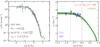 |
Fig. A.1 Structural and kinematical properties for NGC 6101. Left panel: number density profile from de Boer et al. (2019, in gray). Posterior values for the model’s free parameters are reported. The green lines show 1000 model realizations from posterior samples. Right panel: 1D velocity dispersion profile in km s−1. In blue are HST data from Libralato et al. (2022), whereas in purple are Gaia data from Vasiliev & Baumgardt (2021). Velocities were converted assuming the distance from Baumgardt & Vasiliev (2021). The red point shows the σμ obtained from single stars < 0.2Rhl plotted at 0.2Rhl (the number of stars used in the calculation is also reported within square brackets). The vertical lines mark 0.2Rhl, and Rhl with the light-gray band depicting the radial range [0.95; 1.05] Rhl. |
Appendix B Table of values of Δs and velocity dispersion ratios
In this Appendix, we report the results for the GC sample considered in this study. In particular, in Table B.1 we list the values Δobs(< Rhl) and σμ (< 0.2Rhl)/σμ(Rhl) obtained for the sample of 21 clusters with HST coverage of at least one half-light radius (see Sect. 4 for the definition and calculation details of the parameters). Similarly, Table B.2 shows the results (namely Δobs(< 0.7Rhl), and σμ(< 0.2Rhl/σμ(Rhl)) for the nine clusters with HST coverage smaller than one half-light radius.
Properties of the sample of 21 clusters analyzed in this study with FoV larger than Rhl.
Properties of nine clusters with FoV coverage smaller than Rhl.
References
- Alessandrini, E., Lanzoni, B., Ferraro, F. R., Miocchi, P., & Vesperini, E. 2016, ApJ, 833, 252 [NASA ADS] [CrossRef] [Google Scholar]
- Anderson, J., Sarajedini, A., Bedin, L. R., et al. 2008, AJ, 135, 2055 [Google Scholar]
- Andrews, J. J., & Kalogera, V. 2022, ApJ, 930, 159 [NASA ADS] [CrossRef] [Google Scholar]
- Antonini, F., & Rasio, F. A. 2016, ApJ, 831, 187 [Google Scholar]
- Arca Sedda, M., Askar, A., & Giersz, M. 2018, MNRAS, 479, 4652 [NASA ADS] [CrossRef] [Google Scholar]
- Arca Sedda, M., Kamlah, A. W. H., Spurzem, R., et al. 2023, MNRAS, 526, 429 [NASA ADS] [CrossRef] [Google Scholar]
- Arca Sedda, M., Kamlah, A. W. H., Spurzem, R., et al. 2024a, MNRAS, 528, 5119 [NASA ADS] [CrossRef] [Google Scholar]
- Arca Sedda, M., Kamlah, A. W. H., Spurzem, R., et al. 2024b, MNRAS, 528, 5140 [CrossRef] [Google Scholar]
- Aros, F. I., & Vesperini, E. 2023, MNRAS, 525, 3136 [NASA ADS] [CrossRef] [Google Scholar]
- Askar, A., Szkudlarek, M., Gondek-Rosińska, D., Giersz, M., & Bulik, T. 2017, MNRAS, 464, L36 [CrossRef] [Google Scholar]
- Askar, A., Arca Sedda, M., & Giersz, M. 2018, MNRAS, 478, 1844 [NASA ADS] [CrossRef] [Google Scholar]
- Askar, A., Askar, A., Pasquato, M., & Giersz, M. 2019, MNRAS, 485, 5345 [Google Scholar]
- Balbinot, E., Dodd, E., Matsuno, T., et al. 2024, A&A, 687, L3 [NASA ADS] [CrossRef] [EDP Sciences] [Google Scholar]
- Banerjee, S., Baumgardt, H., & Kroupa, P. 2010, MNRAS, 402, 371 [Google Scholar]
- Baumgardt, H., & Vasiliev, E. 2021, MNRAS, 505, 5957 [NASA ADS] [CrossRef] [Google Scholar]
- Baumgardt, H., Sollima, A., & Hilker, M. 2020, PASA, 37, e046 [Google Scholar]
- Belczynski, K., Kalogera, V., & Bulik, T. 2002, ApJ, 572, 407 [NASA ADS] [CrossRef] [Google Scholar]
- Bhat, B., Lanzoni, B., Vesperini, E., et al. 2024, ApJ, 968, 2 [NASA ADS] [CrossRef] [Google Scholar]
- Bianchini, P., van de Ven, G., Norris, M. A., Schinnerer, E., & Varri, A. L. 2016, MNRAS, 458, 3644 [NASA ADS] [CrossRef] [Google Scholar]
- Breen, P. G., & Heggie, D. C. 2013, MNRAS, 432, 2779 [NASA ADS] [CrossRef] [Google Scholar]
- Chakrabarti, S., Simon, J. D., Craig, P. A., et al. 2023, AJ, 166, 6 [NASA ADS] [CrossRef] [Google Scholar]
- Chomiuk, L., Strader, J., Maccarone, T. J., et al. 2013, ApJ, 777, 69 [NASA ADS] [CrossRef] [Google Scholar]
- Dalessandro, E., Ferraro, F. R., Massari, D., et al. 2015, ApJ, 810, 40 [NASA ADS] [CrossRef] [Google Scholar]
- Dalessandro, E., Cadelano, M., Vesperini, E., et al. 2019, ApJ, 884, L24 [Google Scholar]
- de Boer, T. J. L., Gieles, M., Balbinot, E., et al. 2019, MNRAS, 485, 4906 [Google Scholar]
- Di Carlo, U. N., Agrawal, P., Rodriguez, C. L., & Breivik, K. 2024, ApJ, 965, 22 [CrossRef] [Google Scholar]
- Dickson, N., Smith, P. J., Hénault-Brunet, V., Gieles, M., & Baumgardt, H. 2024, MNRAS, 529, 331 [NASA ADS] [CrossRef] [Google Scholar]
- El-Badry, K. 2024, Open J. Astrophys., 7, 38 [NASA ADS] [Google Scholar]
- El-Badry, K., Rix, H.-W., Cendes, Y., et al. 2023a, MNRAS, 521, 4323 [NASA ADS] [CrossRef] [Google Scholar]
- El-Badry, K., Rix, H.-W., Quataert, E., et al. 2023b, MNRAS, 518, 1057 [Google Scholar]
- Ferraro, F. R., Lanzoni, B., Raso, S., et al. 2018, ApJ, 860, 36 [NASA ADS] [CrossRef] [Google Scholar]
- Ferraro, F. R., Lanzoni, B., Dalessandro, E., et al. 2019, Nat. Astron., 3, 1149 [NASA ADS] [CrossRef] [Google Scholar]
- Ferraro, F. R., Lanzoni, B., Vesperini, E., et al. 2023a, ApJ, 950, 145 [NASA ADS] [CrossRef] [Google Scholar]
- Ferraro, F. R., Mucciarelli, A., Lanzoni, B., et al. 2023b, Nature Communications, 14, 2584 [NASA ADS] [CrossRef] [Google Scholar]
- Foreman-Mackey, D., Hogg, D. W., Lang, D., & Goodman, J. 2013, PASP, 125, 306 [Google Scholar]
- Fragione, G., & Kocsis, B. 2018, Phys. Rev. Lett., 121, 161103 [Google Scholar]
- Fregeau, J. M., Cheung, P., Portegies Zwart, S. F., & Rasio, F. A. 2004, MNRAS, 352, 1 [CrossRef] [Google Scholar]
- Gaia Collaboration (Panuzzo, P., et al.) 2024, A&A, 686, L2 [NASA ADS] [CrossRef] [EDP Sciences] [Google Scholar]
- Giacobbo, N., & Mapelli, M. 2020, ApJ, 891, 141 [NASA ADS] [CrossRef] [Google Scholar]
- Gieles, M., & Zocchi, A. 2015, MNRAS, 454, 576 [NASA ADS] [CrossRef] [Google Scholar]
- Giersz, M., & Heggie, D. C. 1996, MNRAS, 279, 1037 [NASA ADS] [Google Scholar]
- Giersz, M., Heggie, D. C., Hurley, J. R., & Hypki, A. 2013, MNRAS, 431, 2184 [NASA ADS] [CrossRef] [Google Scholar]
- Giesers, B., Dreizler, S., Husser, T.-O., et al. 2018, MNRAS, 475, L15 [NASA ADS] [CrossRef] [Google Scholar]
- Heggie, D. C., & Giersz, M. 2014, MNRAS, 439, 2459 [NASA ADS] [CrossRef] [Google Scholar]
- Heggie, D., & Hut, P. 2003, The Gravitational Million-Body Problem: A Multidisciplinary Approach to Star Cluster Dynamics (Cambridge University Press) [Google Scholar]
- Hénon, M. 1971a, Ap&SS, 13, 284 [Google Scholar]
- Hénon, M. H. 1971b, Ap&SS, 14, 151 [Google Scholar]
- Hobbs, G., Lorimer, D. R., Lyne, A. G., & Kramer, M. 2005, MNRAS, 360, 974 [Google Scholar]
- Hong, J., Vesperini, E., Askar, A., et al. 2018, MNRAS, 480, 5645 [NASA ADS] [CrossRef] [Google Scholar]
- Hurley, J. R., Pols, O. R., & Tout, C. A. 2000, MNRAS, 315, 543 [Google Scholar]
- Hurley, J. R., Tout, C. A., & Pols, O. R. 2002, MNRAS, 329, 897 [Google Scholar]
- Hurley, J. R., Sippel, A. C., Tout, C. A., & Aarseth, S. J. 2016, PASA, 33, e036 [NASA ADS] [CrossRef] [Google Scholar]
- Hypki, A., & Giersz, M. 2013, MNRAS, 429, 1221 [NASA ADS] [CrossRef] [Google Scholar]
- Janka, H.-T. 2013, MNRAS, 434, 1355 [Google Scholar]
- King, I. R. 1966, AJ, 71, 64 [Google Scholar]
- Kremer, K., Ye, C. S., Rui, N. Z., et al. 2020, ApJS, 247, 48 [NASA ADS] [CrossRef] [Google Scholar]
- Kroupa, P. 1995, MNRAS, 277, 1491 [Google Scholar]
- Kroupa, P. 2001, MNRAS, 322, 231 [NASA ADS] [CrossRef] [Google Scholar]
- Kroupa, P., Weidner, C., Pflamm-Altenburg, J., et al. 2013, in Planets, Stars and Stellar Systems, 5: Galactic Structure and Stellar Populations, eds. T. D. Oswalt, & G. Gilmore, 115 [CrossRef] [Google Scholar]
- Lanzoni, B., Ferraro, F. R., Alessandrini, E., et al. 2016, ApJ, 833, L29 [NASA ADS] [CrossRef] [Google Scholar]
- Libralato, M., Bellini, A., Vesperini, E., et al. 2022, ApJ, 934, 150 [NASA ADS] [CrossRef] [Google Scholar]
- Maccarone, T. J., Kundu, A., Zepf, S. E., & Rhode, K. L. 2007, Nature, 445, 183 [NASA ADS] [CrossRef] [Google Scholar]
- Mackey, A. D., Wilkinson, M. I., Davies, M. B., & Gilmore, G. F. 2007, MNRAS, 379, L40 [NASA ADS] [CrossRef] [Google Scholar]
- Mackey, A. D., Wilkinson, M. I., Davies, M. B., & Gilmore, G. F. 2008, MNRAS, 386, 65 [NASA ADS] [CrossRef] [Google Scholar]
- Mandel, I. 2016, MNRAS, 456, 578 [Google Scholar]
- Marín Pina, D., Rastello, S., Gieles, M., et al. 2024, A&A, 688, L2 [NASA ADS] [CrossRef] [EDP Sciences] [Google Scholar]
- Miller-Jones, J. C. A., Strader, J., Heinke, C. O., et al. 2015, MNRAS, 453, 3918 [Google Scholar]
- Miocchi, P., Lanzoni, B., Ferraro, F. R., et al. 2013, ApJ, 774, 151 [Google Scholar]
- Moody, K., & Sigurdsson, S. 2009, ApJ, 690, 1370 [NASA ADS] [CrossRef] [Google Scholar]
- Morscher, M., Umbreit, S., Farr, W. M., & Rasio, F. A. 2013, ApJ, 763, L15 [Google Scholar]
- Morscher, M., Pattabiraman, B., Rodriguez, C., Rasio, F. A., & Umbreit, S. 2015, ApJ, 800, 9 [NASA ADS] [CrossRef] [Google Scholar]
- Peuten, M., Zocchi, A., Gieles, M., Gualandris, A., & Hénault-Brunet, V. 2016, MNRAS, 462, 2333 [CrossRef] [Google Scholar]
- Pryor, C., & Meylan, G. 1993, in Astronomical Society of the Pacific Conference Series, 50, Structure and Dynamics of Globular Clusters, eds. S. G. Djorgovski, & G. Meylan, 357 [Google Scholar]
- Raso, S., Ferraro, F. R., Dalessandro, E., et al. 2017, ApJ, 839, 64 [NASA ADS] [CrossRef] [Google Scholar]
- Rastello, S., Iorio, G., Mapelli, M., et al. 2023, MNRAS, 526, 740 [NASA ADS] [CrossRef] [Google Scholar]
- Repetto, S., Davies, M. B., & Sigurdsson, S. 2012, MNRAS, 425, 2799 [Google Scholar]
- Repetto, S., Igoshev, A. P., & Nelemans, G. 2017, MNRAS, 467, 298 [Google Scholar]
- Rodriguez, C. L., Morscher, M., Pattabiraman, B., et al. 2015, Phys. Rev. Lett., 115, 051101 [Google Scholar]
- Rodriguez, C. L., Haster, C.-J., Chatterjee, S., Kalogera, V., & Rasio, F. A. 2016a, ApJ, 824, L8 [NASA ADS] [CrossRef] [Google Scholar]
- Rodriguez, C. L., Zevin, M., Pankow, C., Kalogera, V., & Rasio, F. A. 2016b, ApJ, 832, L2 [NASA ADS] [CrossRef] [Google Scholar]
- Rodriguez, C. L., Amaro-Seoane, P., Chatterjee, S., et al. 2018, Phys. Rev. D, 98, 123005 [NASA ADS] [CrossRef] [Google Scholar]
- Samsing, J., & D’Orazio, D. J. 2018, MNRAS, 481, 5445 [NASA ADS] [CrossRef] [Google Scholar]
- Samsing, J., Askar, A., & Giersz, M. 2018, ApJ, 855, 124 [NASA ADS] [CrossRef] [Google Scholar]
- Sarajedini, A., Bedin, L. R., Chaboyer, B., et al. 2007, AJ, 133, 1658 [Google Scholar]
- Sippel, A. C., & Hurley, J. R. 2013, MNRAS, 430, L30 [NASA ADS] [Google Scholar]
- Spitzer, L. 1987, Dynamical evolution of globular clusters (Princeton, NJ: Princeton University Press) [Google Scholar]
- Strader, J., Chomiuk, L., Maccarone, T. J., Miller-Jones, J. C. A., & Seth, A. C. 2012, Nature, 490, 71 [NASA ADS] [CrossRef] [Google Scholar]
- Tanikawa, A., Hattori, K., Kawanaka, N., et al. 2023, ApJ, 946, 79 [CrossRef] [Google Scholar]
- Tanikawa, A., Cary, S., Shikauchi, M., Wang, L., & Fujii, M. S. 2024a, MNRAS, 527, 4031 [Google Scholar]
- Tanikawa, A., Wang, L., & Fujii, M. S. 2024b, arXiv e-prints [arXiv:2407.03662] [Google Scholar]
- Torniamenti, S., Gieles, M., Penoyre, Z., et al. 2023, MNRAS, 524, 1965 [NASA ADS] [CrossRef] [Google Scholar]
- Trager, S. C., King, I. R., & Djorgovski, S. 1995, AJ, 109, 218 [NASA ADS] [CrossRef] [Google Scholar]
- Vasiliev, E., & Baumgardt, H. 2021, MNRAS, 505, 5978 [NASA ADS] [CrossRef] [Google Scholar]
- Weatherford, N. C., Chatterjee, S., Rodriguez, C. L., & Rasio, F. A. 2018, ApJ, 864, 13 [NASA ADS] [CrossRef] [Google Scholar]
- Weatherford, N. C., Chatterjee, S., Kremer, K., & Rasio, F. A. 2020, ApJ, 898, 162 [NASA ADS] [CrossRef] [Google Scholar]
- WFIRST Astrometry Working Group (Sanderson, R. E., et al.) 2019, J. Astron. Telesc. Instrum. Syst., 5, 044005 [NASA ADS] [Google Scholar]
- Zevin, M., Samsing, J., Rodriguez, C., Haster, C.-J., & Ramirez-Ruiz, E. 2019, ApJ, 871, 91 [NASA ADS] [CrossRef] [Google Scholar]
- Zocchi, A., Gieles, M., & Hénault-Brunet, V. 2019, MNRAS, 482, 4713 [Google Scholar]
The name MOCCA stands for MOnte Carlo Cluster simulAtor, see https://moccacode.net/
Following what is commonly done in PM studies, we used the two velocity components projected on the plane of the sky to determine the radial (σR) and tangential (σT) velocity dispersions for each cluster. We then defined ![Mathematical equation: $\[\sigma_\mu^2 \equiv\left(\sigma_{\mathrm{R}}^2+\sigma_{\mathrm{T}}^2\right) / 2\]$](/articles/aa/full_html/2024/10/aa50954-24/aa50954-24-eq38.png) .
.
Computed from stars with projected distance from the center ∈ [0.95; 1.05] Rhl.
Publicy available at https://archive.stsci.edu/hlsp/hacks
The catalog is publicly available at https://people.smp.uq.edu.au/HolgerBaumgardt/globular/. Values used in this work are from the 4th version of the catalog updated in March 2023.
Full documentation available at https://emcee.readthedocs.io/en/stable/
Publicy available at https://github.com/mgieles/limepy
For NGC 6144 we applied slightly different selections, adopting the 5th and 95th quantiles for the color-magnitude diagram and QFIT selections. Indeed, we found that the previous selections introduced systematics in the spatial distribution of the brightest stars thereby biasing the calculation of mass-segregation proxies through the nCRDs.
All Tables
Properties of the sample of 21 clusters analyzed in this study with FoV larger than Rhl.
All Figures
|
Fig. 1 Simulation properties at 13 Gyr, each point representing a different simulation. Moving downwards on the y-axis: luminosity density (in units of L⊙ per2), core to half-light radius ratio (Rc/Rhl), dynamical age (nh), inverse of the equipartition mass, μ(< 0.1Rhl), BH mass fraction (Mbh/MGC), and mass segregation parameter Δ. Simulations are color-coded according to the number of BHs (NBH) at 13 Gyr. A value of log NBH = −0.5 was assigned to those with no BHs. Similarly, simulations that do not retain any BH at 13 Gyr are shown at MBH/MGC = 5 × 10⁻⁶ on the bottom row for visualization purposes only. |
| In the text | |
|
Fig. 2 BH mass fraction as a function of Δ. Colors depict the number of BHs in the simulation at 13 Gyr, while different symbols show the adopted fallback prescription in the initial conditions. Simulations without BHs at 13 Gyr are shown at MBH/MGC = 5 × 10⁻⁶. To account for fluctuations in the estimates arising due to the discrete nature of the simulations, we performed 500 different projections along the LOS, and for each of them, we measured Δ. The values shown are the median ones. Errors obtained computing the 16% and 84% percentiles of the distribution are also shown although barely visible. |
| In the text | |
|
Fig. 3 Mass segregation parameter as a function of the velocity dispersion ratio. Symbols show whether the simulation had (diamond) or had not (upside-down triangle) the fallback prescription for BH formation. Different colors depict the BH mass fraction (see the color bar on the side) Finally, error bars were obtained from multiple projections along the LOS. |
| In the text | |
|
Fig. 4 Photometric completeness for NGC 6584. Left panel: two-dimensional map of sources in the magnitude range [VTO + 2; VTO + 3], with VTO being the turn-off magnitude. Each star is color-coded according to the completeness in the V band. Right panel: V-magnitude dependence of the photometric completeness. Stars are color-coded according to their projected distance from the center normalized to Rhl. The gray area marks c < 0.5 whereas the blue region shows the [VTO + 2; Vto + 3] magnitude range. |
| In the text | |
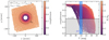 |
Fig. 5 Same as Fig. 4 for NGC 7089. |
| In the text | |
|
Fig. 6 BH mass fraction as a function of Δobs(< Rhl) (left panel) and Δobs(< 0.7Rhl) (right panel). Points show the simulation properties recomputed according to the magnitude and spatial selections adopted for the observations (see Sect. 4.1), whereas the vertical red lines show values obtained for the Galactic GCs studied in this work (along with errors as shaded areas). Simulations without BHs at 13 Gyr are shown at MBH/MGC = 5 × 10⁻⁶. |
| In the text | |
|
Fig. 7 Δobs(< Rhl) (left panel) and Δobs(< 0.7Rhl) (right panel) as a function of the velocity dispersion ratio. Values from the simulations were recomputed according to the magnitude and spatial selections adopted for the observations (see Sect. 4.1). Simulations are color-coded according to the BH mass fraction (see the color bar). Error bars were computed from multiple LOS projections. Finally, in blue we show the values (along with error bars) obtained for Galactic GCs (see Sect. 4 for details). The observations shown in this plot are reported in Tables B.1 and B.2. |
| In the text | |
|
Fig. A.1 Structural and kinematical properties for NGC 6101. Left panel: number density profile from de Boer et al. (2019, in gray). Posterior values for the model’s free parameters are reported. The green lines show 1000 model realizations from posterior samples. Right panel: 1D velocity dispersion profile in km s−1. In blue are HST data from Libralato et al. (2022), whereas in purple are Gaia data from Vasiliev & Baumgardt (2021). Velocities were converted assuming the distance from Baumgardt & Vasiliev (2021). The red point shows the σμ obtained from single stars < 0.2Rhl plotted at 0.2Rhl (the number of stars used in the calculation is also reported within square brackets). The vertical lines mark 0.2Rhl, and Rhl with the light-gray band depicting the radial range [0.95; 1.05] Rhl. |
| In the text | |
Current usage metrics show cumulative count of Article Views (full-text article views including HTML views, PDF and ePub downloads, according to the available data) and Abstracts Views on Vision4Press platform.
Data correspond to usage on the plateform after 2015. The current usage metrics is available 48-96 hours after online publication and is updated daily on week days.
Initial download of the metrics may take a while.