| Issue |
A&A
Volume 688, August 2024
|
|
|---|---|---|
| Article Number | L2 | |
| Number of page(s) | 5 | |
| Section | Letters to the Editor | |
| DOI | https://doi.org/10.1051/0004-6361/202450460 | |
| Published online | 30 July 2024 | |
Letter to the Editor
Dynamical formation of Gaia BH3 in the progenitor globular cluster of the ED-2 stream
1
Departament de Física Quàntica i Astrofísica, Institut de Ciències del Cosmos, Universitat de Barcelona, Martí i Franquès 1, 08028 Barcelona, Spain
e-mail: danielmarin@icc.ub.edu
2
ICREA, Pg. Lluís Companys 23, 08010 Barcelona, Spain
3
TAPIR, California Institute of Technology, Pasadena, CA 91125, USA
Received:
21
April
2024
Accepted:
7
July
2024
Context. The star–black hole (S–BH) binary known as Gaia BH3, discovered by the Gaia Collaboration is chemically and kinematically associated with the metal-poor ED-2 stream in the Milky Way halo.
Aims. We explore the possibility that Gaia BH3 was assembled dynamically in the progenitor globular cluster (GC) of the ED-2 stream.
Methods. We used a public suite of star-by-star dynamical Monte Carlo models to identify S–BH binaries in GCs with different initial masses and (half-mass) radii.
Results. We show that a likely progenitor of the ED-2 stream was a relatively low-mass (≲105 M⊙) GC with an initial half-mass radius of ∼4 pc. Such a GC can dynamically retain a large fraction of its BH population and dissolve on the orbit of ED-2. From the suite of models we find that GCs produce ∼3 − 30 S–BH binaries, approximately independently of initial GC mass and inversely correlated with initial cluster radius. Scaling the results to the Milky Way GC population, we find that ∼75% of the S–BH binaries formed in GCs are ejected from their host GC, all in the early phases of evolution (≲1 Gyr); these are expected to no longer be close to streams. The ∼25% of S–BH binaries retained until dissolution are expected to form part of streams, such that for an initial mass of the progenitor of ED-2 of a few 104 M⊙, we expect ∼2 − 3 S–BH to end up in the stream. GC models with metallicities similar to Gaia BH3 (≲1% solar) include S–BH binaries with similar BH masses (≳30 M⊙), orbital periods, and eccentricities.
Conclusion. We predict that the Galactic halo contains of order 105 S–BH binaries that formed dynamically in GCs, a fraction of which may readily be detected in Gaia DR4. The detection of these sources provides valuable tests of BH dynamics in clusters and their contribution to gravitational wave sources.
Key words: stars: black holes / stars: Population II / globular clusters: general / Galaxy: halo / Galaxy: kinematics and dynamics
© The Authors 2024
 Open Access article, published by EDP Sciences, under the terms of the Creative Commons Attribution License (https://creativecommons.org/licenses/by/4.0), which permits unrestricted use, distribution, and reproduction in any medium, provided the original work is properly cited.
This article is published in open access under the Subscribe to Open model. Subscribe to A&A to support open access publication.
1. Introduction
The discovery of a star–black hole (S–BH) binary, known as Gaia BH3, by the Gaia collaboration (Gaia Collaboration 2024) provides a novel glimpse into the population of dormant BHs. Gaia BH3 is composed of a 33 M⊙ BH with a 0.76 M⊙ star. The star is a metal-poor giant, with [Fe/H] ≃ −2.6. The binary has an eccentricity of e ≃ 0.73, and a wide orbit with period P ≃ 4250 d. Gaia BH3 is on a halo orbit, similar to the debris of the Sequoia accretion event.
The previously discovered Gaia BH1 (El-Badry et al. 2023b) is a binary with a Sun-like star orbiting a BH with a mass mBH ≃ 10 M⊙, an eccentricity e = 0.45, and a period of P ≃ 186 d. Gaia BH2 (El-Badry et al. 2023a) is a binary with a red giant orbiting a mBH ≃ 9 M⊙ BH, with an eccentricity e ≃ 0.5, and a relatively long period of P ≃ 1280 d. Their metallicities ([Fe/H] ≃ −0.2) and their inferred orbits in the Galactic plane point towards a formation in a young stellar population, possibly an open cluster (Rastello et al. 2023; Di Carlo et al. 2024; Tanikawa et al. 2024a; Arca Sedda et al. 2024) or an isolated stellar binary (Kotko et al. 2024).
The association of Gaia BH3 with the stellar halo calls for another formation scenario. Under the assumption that the unseen companion is a single BH1, Gaia Collaboration (2024) argue that the formation of Gaia BH3 in isolation is unlikely (but see El-Badry 2024; Iorio et al. 2024). The star does not present strong chemical peculiarities, indicating a lack of pollution by the BH progenitor in its evolved stage. This makes a dynamical formation scenario, where the system is assembled after the BH progenitor has exploded as a supernova, more plausible. Its orbit in the Galactic halo and low metallicity suggest that Gaia BH3 formed in a globular cluster (GC).
Balbinot et al. (2024) show that Gaia BH3 is both chemically and kinematically associated with the ED-2 stream (Dodd et al. 2023). The progenitor of the ED-2 stream was most likely a GC, given its low velocity-dispersion (Balbinot et al. 2023) and the absence of an [Fe/H] spread (< 0.04 dex, Balbinot et al. 2024). These authors also find a negligible spread in Na and Al, suggesting an initial cluster mass ≲5 × 10⁴ M⊙. The fact that the cluster is dissolved also provides a mass limit: using the results of Gieles & Gnedin (2023) we find that the maximum initial mass of a cluster with BHs that can dissolve in 13 Gyr on the orbit of ED-2 is ∼9 × 10⁴ M⊙.
To date, only two (possibly three) detached stellar-mass BH binary candidates have been found in GCs (in NGC 3201, Giesers et al. 2018, 2019)2. Only line-of-sight velocities are available for these binaries, providing a minimum BH mass of ≳5 M⊙. Kremer et al. (2018b) showed that these binaries were likely formed and shaped via dynamical exchange interactions. Finding evidence for massive BHs (≳30 M⊙) in a (dissolved) GC is critical to understanding the contribution of dynamically produced BBHs to the growing sample of gravitational wave sources (e.g., Portegies Zwart & McMillan 2000; Rodriguez et al. 2016; Askar et al. 2017; Antonini et al. 2023).
In this Letter we show that Gaia BH3 could have formed dynamically in the progenitor GC of the ED-2 stream.
2. Methods
We used the suite of GC simulations run with the Cluster Monte Carlo (CMC) code. CMC is a Hénon-type Monte Carlo code for the long-term evolution of collisional stellar systems (Rodriguez et al. 2022, and references therein). The integration is done on a star-by-star basis, following gravitational interactions, the internal evolution of stars and binary stars, strong few-body interactions, and dynamical ejections (Weatherford et al. 2023). Further details on the code can be found in Rodriguez et al. (2022).
For this work we used the set of 148 CMC models presented in Kremer et al. (2020). This catalogue is meant to sample the relevant parameter space of local-Universe GCs varying the following initial conditions: the number of stars N, virial radius rv,3 metallicity Z, and Galactocentric distance RG. The choice of values for the above parameters is N ∈ [2, 4, 8, 16]×105, rv ∈ [0.5, 1, 2, 4] pc, Z ∈ [0.0002, 0.002, 0.02], and RG ∈ [2, 8, 20] kpc, which account for 144 models, plus four extra models with N = 3.2 × 10⁶, RG = 20 kpc, Z ∈ [0.0002, 0.02], and rv ∈ [1, 2] pc. All models adopt a Kroupa (2001) stellar mass function in the range 0.08 − 150 M⊙, resulting in an initial mean mass of 0.6 M⊙.
We first looked at the raw results of all S–BH occurring in the database (see Sect. 3). We also made the CMC database representative for the Milky Way GC system, by applying weights to the result of GCs with different N by a factor N−1, such that the logarithmically spaced N values represent an initial GC mass function of the form  . We then only considered the low-metallicity models (Z = 2 × 10⁻⁴ and Z = 2 × 10⁻³), with relative weights 4:1, representative of the Milky Way GC population (e.g., Harris 1996). We considered equal contributions of the different rv and RG models.
We only considered hard binaries (Heggie 1975), defined as those whose absolute value of the binding energy is greater than the average kinetic energy of particles in the GC core. This was done to exclude loosely bound pairs that are constantly being assembled and destroyed.
All models were evolved until 14 Gyr, or until dissolution if that occured before 14 Gyr. As clusters evolve they lose mass and stars due to stellar evolution, internal two-body relaxation, and interactions with the Galactic tidal field. Therefore, GCs dissolve over a period that depends on their mass and RG. A cluster is considered dissolved when the number of particles drops below ∼104 (see Sect. 2.3 of Kremer et al. 2020, for the exact definition). Of the 148 models in the catalogue, 21 of them dissolved, mostly those with low masses at small Galactocentric radii (see Table 6 in Kremer et al. 2020 for the list of dissolved models).
3. Origin of Gaia BH3-like binaries
In this section we explore the formation of S–BH binaries in the CMC catalogue that are the most similar to Gaia BH3. From the 1837 unique S–BH binaries in the catalogue, we removed 424 accreting binaries. The remaining 1413 detached binaries are shown in Fig. 1, where the contribution of each of the models is weighted as explained in Sect. 2. From these binaries, 78% were ejected and the rest remain in the cluster. We assume that the S–BH binaries that survive until 14 Gyr in surviving clusters remain in these clusters until dissolution, which is justified by the fact that most binaries form within approximately the first gigayear.
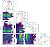 |
Fig. 1. Probability distribution functions for the masses of the BH and star (mBH and m⋆, respectively) and orbital parameters (period P and eccentricity e) for all the detached S–BH binaries in the cluster simulations of Kremer et al. (2020). For ejected binaries, we show their parameters at the time of ejection. The contribution of each binary to the histogram is weighted as explained in Sect. 2. Shown in red (continuous line for 1D histograms, star symbol for 2D histograms) are the values for Gaia BH3. The dashed red line gives the range for the analysis of Gaia BH3-like binaries in Sect. 3. The green lines in the 1D histogram include only the S–BH binaries that were not ejected from their parent cluster. |
From the sample of detached binaries, we selected those most similar to Gaia BH3, which we define as those whose parameters all fall within the red dashed lines in the subplots of Fig. 1. The red lines span the following ranges: mBH ∈ [25, 45] M⊙, m⋆ ∈ [0.2, 1] M⊙, P ∈ [400, 40000] d, and e ∈ [0.5, 0.9]. These ranges are larger than the typical uncertainties on the observationally inferred parameters of Gaia BH3, which are of order 1–2%, and were chosen to (i) cover a roughly similar fraction of the ranges of the parameters found in the models and (ii) end up with a reasonable number of S–BH binaries. These criteria selected 20 binaries. Next we refined this sample to match the model GC properties with what we know of the ED-2 stream, but before doing so, it is worth noting that Gaia BH3-like binaries exist and that all of them have a dynamical origin.
From the 20 resembling S–BH binaries, there were 15 ejected binaries and 5 binaries that remained in the cluster until dissolution. We refer to these five candidate Gaia BH3-like binaries as cSBH1-5. For these candidates, the masses of the components are mBH = [29.9, 40.5, 34.8, 32.0, 29.6] M⊙ and m⋆ = [0.21, 0.44, 0.31, 0.22, 0.65] M⊙. The semi-major axes are a = [69, 57, 57, 64, 27] AU (which imply periods of P = [38, 25, 27, 33, 9]×103 d) and the eccentricities are e = [0.72, 0.80, 0.61, 0.86, 0.58]. All candidate binaries originate from cluster models with initial parameters rv = 4 pc and RG = 2 kpc. The large rv results because clusters with low density can dynamically retain many of their BHs, which in turn leads to efficient stream formation (Gieles et al. 2021; Roberts et al. 2024). The binaries cSBH1-3 originate from the model with initial N = 2 × 10⁵, whereas cSBH4 and cSBH5 originate in the models with N = 4 × 10⁵ and N = 8 × 10⁵, respectively. If we apply the weights of the GC initial mass function (Sect. 2), we find that three-fourths of the S–BH binaries come from the N = 2 × 10⁵ models. The corresponding initial mass (∼105 M⊙) is within a factor of ∼2 of the mass estimate provided by Balbinot et al. (2024). Combined with the upper limits from the abundances and dissolution time (Sect. 1), we therefore conclude that the models favour an initial GC mass ≲105 M⊙. As expected from the high BH masses, all candidate binaries form in the lowest metallicity model, Z = 0.0002, except for cSBH3, which has Z = 0.002 and mBH grew by a stellar collision of its progenitor.
Binaries cSBH1 and cSBH2 form dynamically about 100 Myr after GC formation, corresponding to the moment of core collapse of the BH subsystem. The classic picture is that a binary forms in a three-body interaction (Heggie 1975; Atallah et al. 2024). The outcome of core collapse is the production of a dynamically active BBH, likely involving between five and ten particles (Tanikawa et al. 2012). The S–BH appears to form in an intermediate step, involving two stars and a BH, and it seems to be a byproduct of BBH formation. In the case of cSBH1, it is directly formed in a three-body interaction, whereas cSBH2 is the exchange of two three-body binaries. Developing a full understanding of the relation between the formation of the S–BH and the BBH is beyond the scope of this work. We simply note here that it is a curiosity worth looking into in future work, and in Sect. 4.3 we discuss the implications. Binaries cSBH3-5 form in three-body interactions but at later times, around ∼1 Gyr. After formation, all candidate binaries undergo several strong interactions (∼3 − 18), implying that even if formed from isolated binary evolution (El-Badry 2024; Iorio et al. 2024), dynamical interactions in the ED-2 progenitor need to be included to understand their final properties.
If we consider the 15 Gaia BH3-like ejected binaries, we also find that most of them form in three-body interactions. After formation, each of the ejected binaries undergoes multiple strong interactions (∼1 − 12) until it is ejected, which most do following an interaction with a BBH, which are frequent in clusters with few BHs (Marín Pina & Gieles 2024).
4. Implications
4.1. Formation efficiency
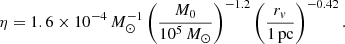
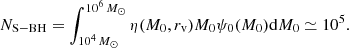
We now compute how many S–BH binaries are expected to be produced by the ED-2 stream. We begin by defining the formation efficiency, η, as the total number (i.e., ejected and retained) of S–BH binaries that form in a cluster per unit of M0. We find a clear dependence of η on M0 and rv, shown in Fig. 2. The formation efficiency is higher in denser and less massive clusters; however, this trend does not extend to lower masses (≲104 M⊙). There, it levels off as there is a hard limit where the number of ejected S–BH binaries, NS − BH, equals the initial number of BHs in the cluster, NBH (see also Fig. 1 in Tanikawa et al. 2024b). For more massive clusters, the formation of S–BH binaries is relatively inhibited by pronounced dynamical heating from their large central BH populations (Kremer et al. 2018a). In the CMC regime, the formation efficiency can be approximated by the following power law:
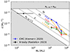 |
Fig. 2. Formation efficiency of S–BH in all CMC models with Z = 2 × 10⁻⁴ (bullets) and all S–BH formed in the N-body models of Rastello et al. (2023) for solar metallicity (square). The dashed lines show the maximum η, corresponding to all BHs in the cluster being in a S–BH, and the minimum η, corresponding to clusters with one BH. The dotted lines correspond to constant numbers of S–BH. |
Extrapolating to the mass estimate for the ED-2 progenitor (5 × 10⁴ M⊙, Sect. 1) and rv = 2 − 4 pc, implies that the ED-2 stream produced ∼9 − 13 S–BH binaries, of which ∼2 − 3 remain in the progenitor cluster until dissolution. We conclude that the dynamical formation of Gaia BH3 is a viable explanation for its origin.
4.2. Number of S–BH in the Galactic halo
With the relation η(M0, rv) from Eq. (1) we can estimate the total number of S–BH binaries produced dynamically in the complete population of Galactic GCs. We write the initial GC mass function (GCMF) as  . We then assume that all clusters lose 40% of their mass by stellar evolution and an amount Δ ≃ 2 × 10⁵ M⊙ by evaporation. This amount is required to obtain the turn-over mass in the GCMF at ∼2 × 10⁵ M⊙ if mass is lost at a rate that is constant in time (Jordán et al. 2007). The evolved GCMF can then be written as ψ(M) = μsevA(M + Δ)−2, where μsev ≃ 0.6. The normalisation constant A is found from the total number of Milky Way GCs (157) and integrating ψ(M) from 102 M⊙ (roughly the lowest mass Milky Way GC) to 106 M⊙. The total number of S–BH binaries produced by all Milky Way GCs, including the dissolved ones, is then
Here we weighed the results for different rv equally. We note that there are no CMC models in the range 104 ≤ M0/M⊙ ≲ 105, so the results depend on an extrapolation outside the range of the CMC grid. From the models of lower mass clusters of Rastello et al. (2023) (Fig. 2), this seems reasonable for rv ≳ 1 pc.
Because most S–BH are produced by low-mass dissolved GCs, the number density of S–BH in the Galactic halo follows the initial density distribution of GCs in the Milky Way:  between 1 kpc and 100 kpc (e.g., Fall & Zhang 2001; Gieles & Gnedin 2023). Scaling this to a total number of 105, we then find that at the solar radius the number density of S–BH in the halo is nS−BH ≃ 1 kpc−3, corresponding to ∼1 within the distance to Gaia BH3. Within a distance of 1 − 3 kpc from the Sun there are 5 − 130 S–BH expected from (dissolved) GCs. We note that we predict that the ED-2 progenitor cluster has produced ∼9–13 S–BH binaries, of which ∼2–3 are expected to remain in the stream. The number of nS−BH ≃ 1 kpc−3 corresponds to an average, and does not take into account the close proximity of the ED-2 stream.
4.3. Connecting to gravitational wave sources
As the catalogue of BBH mergers detected via gravitational waves by LIGO/Virgo/KAGRA (LVK) grows (Abbott et al. 2023), the details of the astrophysical origin of these sources remain elusive. Dynamical formation within GCs has emerged as one possible scenario and has been studied at length using N-body cluster simulations, including CMC (e.g., Rodriguez et al. 2016). In GCs, the dynamical formation of S–BH binaries like Gaia BH3 and the three BH candidates observed in NGC 3201 is an inevitable byproduct of the same processes that lead to formation of merging BH pairs (e.g., Kremer et al. 2018b). Thus, the detection of sources like Gaia BH3 provides important constraints on the properties of BHs in clusters, their dynamics, and the role of GCs in forming GW sources.
In Fig. 3 we show the cumulative distribution of BH masses from our CMC models for BHs undergoing BH mergers (grey) and BHs found in S–BH binaries (blue; including both retained and ejected binaries), again adopting the cluster weighting scheme from Sect. 2. For reference, we also show distributions of known stellar-mass BHs with mass measurements: low- and high-mass X-ray binaries (red curve) taken from (Remillard & McClintock 2006; Corral-Santana et al. 2016), BH mergers (black curve) from GWTC-3 (Abbott et al. 2023), and the three Gaia BH3 binaries. The X-ray binary and GW distributions shown in Fig. 3 are raw data and do not take into account detection biases or astrophysical weighting (for discussion, see Fishbach & Kalogera 2022). Figure 3, therefore, does not suggest that the CMC models predict the observed distribution of X-ray binaries, GW sources, or S–BH binaries, merely that the dynamically active populations of BHs in the CMC models have masses similar to both the LVK sources and Gaia BH3. Future discoveries of S–BH binaries in the Milky Way, as well as detailed detectability analysis in the CMC models, can provide constraints on the connection between these populations.
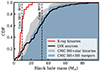 |
Fig. 3. Cumulative distribution of measured BH masses observed as X-ray binaries (Remillard & McClintock 2006; Corral-Santana et al. 2016) and as GW sources (Abbott et al. 2023) compared to distributions of BH masses identified in our CMC models. The vertical dashed lines show measured masses for the three Gaia BHs. |
5. Discussion
5.1. Binary fraction
The prediction of the number of S–BH binaries might be a lower limit due to the relatively low primordial binary fraction in the CMC models (5%). For solar-type stars the initial binary/multiplicity fraction is likely higher (30–40% Moe & Di Stefano 2017). This results in a higher rate of binary-binary interactions providing an additional pathway to formation of S–BH in exchange interactions (e.g., González et al. 2021; Tanikawa et al. 2024a).
5.2. Validity of the CMC catalogue
The mass estimate of the progenitor cluster in the ED-2 stream, ∼5 × 10⁴ M⊙ (Balbinot et al. 2024), is lower than the least massive GC model in our catalogue (1.2 × 10⁵ M⊙), so our results are based on extrapolation. However, they are within the same order of magnitude, so we expect that the values hold if we consider slightly lower cluster masses. Furthermore, the Hénon-type CMC code is unable to resolve strict cluster dissolution, so the properties of the remaining binaries may change. Both points can be addressed with direct N-body models of the ED-2 progenitor.
5.3. Stellar masses and detectability
The stellar masses in the overall population of S–BH in the CMC models peaks at relatively low masses (∼0.2 M⊙), which makes the majority of these S–BH difficult to detect. Recent analyses of the stellar mass function Milky Way GCs (Baumgardt et al. 2023; Dickson et al. 2023) suggest that the low-mass end of the mass function could be flatter than is assumed in CMC. This would lead to higher stellar masses in S–BH binaries. Estimating this effect requires additional dynamical modelling and is beyond the scope of this work (see Weatherford et al. 2021, for preliminary efforts).
5.4. Alternative pathways for Gaia BH3-like binary formation
Recent work suggests that Gaia BH3-like objects may form via isolated binary evolution (El-Badry 2024; Iorio et al. 2024). Although these models can accommodate the binary’s intrinsic properties (including the lack of chemical pollution), they require a natal kick that is incompatible with Gaia BH3 being associated to the ED-2 stream (El-Badry 2024) (but see Iorio et al. 2024 for alternative conclusions based on different stellar models). Although this argues for dynamical formation, the isolated channel is a promising additional pathway to S–BH formation. Our estimate of the dynamical production rates at RG ≃ 8 kpc is only a factor of ∼3 − 10 higher than the isolated production rate of Iorio et al. (2024), with the key difference being their radial distribution in the Galaxy. The dynamical formation scenario predicts that S–BH binaries follow the initial density distribution of GCs,  , whereas an isolated formation scenario predicts that these objects follow the shallower density profile of the stellar halo.
6. Conclusions
In this Letter we studied the dynamical formation of Gaia BH3-like binaries in GCs. We analysed the public catalogue of star-by-star GC simulations in Kremer et al. (2020), and compared it to Gaia BH3. We found that the properties of Gaia BH3 (masses, period, eccentricity and lack of chemical pollution) are compatible with it being assembled dynamically from a previously unbound star and a BH that have not undergone joint stellar evolution.
Furthermore, we extended our analysis to the whole ED-2 stream in particular and the Galactic halo in general. We predict that the stream produced ∼9 − 13 dynamically assembled S–BH binaries, whereas the halo contains ∼105 S–BH binaries, preferentially towards the Galactic centre. The next Gaia data release (DR4, late 2025) will allow us to test this prediction.
Additional BH candidates have been found in GCs as accreting sources via their X-ray/radio emission (e.g., Maccarone et al. 2007; Strader et al. 2012; Miller-Jones et al. 2015).
Acknowledgments
The authors thank Eduardo Balbinot for discussions on ED-2, Newlin Weatherford for useful feedback on the preprint, and the Gaia group at ICCUB for useful interactions. DMP and MG acknowledge financial support from the grants PID2021-125485NB-C22, EUR2020-112157, CEX2019-000918-M funded by MCIN/AEI/10.13039/501100011033 (State Agency for Research of the Spanish Ministry of Science and Innovation) and SGR-2021-01069 (AGAUR). SR acknowledges support from the Beatriu de Pinós postdoctoral program under the Ministry of Research and Universities of the Government of Catalonia (Grant Reference No. 2021 BP 00213). Support for KK was provided by NASA through the NASA Hubble Fellowship grant HST-HF2-51510 awarded by the Space Telescope Science Institute, which is operated by the Association of Universities for Research in Astronomy, Inc., for NASA, under contract NAS5-26555.
References
- Abbott, R., Abbott, T. D., Acernese, F., et al. 2023, Phys. Rev. X, 13, 041039 [Google Scholar]
- Antonini, F., Gieles, M., Dosopoulou, F., & Chattopadhyay, D. 2023, MNRAS, 522, 466 [NASA ADS] [CrossRef] [Google Scholar]
- Arca Sedda, M., Kamlah, A. W. H., Spurzem, R., et al. 2024, MNRAS, 528, 5119 [NASA ADS] [CrossRef] [Google Scholar]
- Askar, A., Szkudlarek, M., Gondek-Rosińska, D., Giersz, M., & Bulik, T. 2017, MNRAS, 464, L36 [CrossRef] [Google Scholar]
- Atallah, D., Weatherford, N. C., Trani, A. A., & Rasio, F. 2024, arXiv e-prints [arXiv:2402.12429] [Google Scholar]
- Balbinot, E., Helmi, A., Callingham, T., et al. 2023, A&A, 678, A115 [NASA ADS] [CrossRef] [EDP Sciences] [Google Scholar]
- Balbinot, E., Dodd, E., Matsuno, T., et al. 2024, A&A, 687, L3 [NASA ADS] [CrossRef] [EDP Sciences] [Google Scholar]
- Baumgardt, H., Hénault-Brunet, V., Dickson, N., & Sollima, A. 2023, MNRAS, 521, 3991 [CrossRef] [Google Scholar]
- Corral-Santana, J. M., Casares, J., Muñoz-Darias, T., et al. 2016, A&A, 587, A61 [NASA ADS] [CrossRef] [EDP Sciences] [Google Scholar]
- Di Carlo, U. N., Agrawal, P., Rodriguez, C. L., & Breivik, K. 2024, ApJ, 965, 22 [CrossRef] [Google Scholar]
- Dickson, N., Hénault-Brunet, V., Baumgardt, H., Gieles, M., & Smith, P. J. 2023, MNRAS, 522, 5320 [NASA ADS] [CrossRef] [Google Scholar]
- Dodd, E., Callingham, T. M., Helmi, A., et al. 2023, A&A, 670, L2 [NASA ADS] [CrossRef] [EDP Sciences] [Google Scholar]
- El-Badry, K. 2024, Open J. Astrophys., 7, 38 [NASA ADS] [Google Scholar]
- El-Badry, K., Rix, H.-W., Cendes, Y., et al. 2023a, MNRAS, 521, 4323 [NASA ADS] [CrossRef] [Google Scholar]
- El-Badry, K., Rix, H.-W., Quataert, E., et al. 2023b, MNRAS, 518, 1057 [Google Scholar]
- Fall, S. M., & Zhang, Q. 2001, ApJ, 561, 751 [NASA ADS] [CrossRef] [Google Scholar]
- Fishbach, M., & Kalogera, V. 2022, ApJ, 929, L26 [NASA ADS] [CrossRef] [Google Scholar]
- Gaia Collaboration (Panuzzo, P., et al.) 2024, A&A, 686, L2 [NASA ADS] [CrossRef] [EDP Sciences] [Google Scholar]
- Gieles, M., & Gnedin, O. Y. 2023, MNRAS, 522, 5340 [NASA ADS] [CrossRef] [Google Scholar]
- Gieles, M., Erkal, D., Antonini, F., Balbinot, E., & Peñarrubia, J. 2021, Nat. Astron., 5, 957 [NASA ADS] [CrossRef] [Google Scholar]
- Giesers, B., Dreizler, S., Husser, T.-O., et al. 2018, MNRAS, 475, L15 [NASA ADS] [CrossRef] [Google Scholar]
- Giesers, B., Kamann, S., Dreizler, S., et al. 2019, A&A, 632, A3 [NASA ADS] [CrossRef] [EDP Sciences] [Google Scholar]
- González, E., Kremer, K., Chatterjee, S., et al. 2021, ApJ, 908, L29 [CrossRef] [Google Scholar]
- Harris, W. E. 1996, AJ, 112, 1487 [Google Scholar]
- Heggie, D. C. 1975, MNRAS, 173, 729 [NASA ADS] [CrossRef] [Google Scholar]
- Iorio, G., Torniamenti, S., Mapelli, M., et al. 2024, A&A, submitted [arXiv:2404.17568] [Google Scholar]
- Jordán, A., McLaughlin, D. E., Côté, P., et al. 2007, ApJS, 171, 101 [CrossRef] [Google Scholar]
- Kotko, I., Banerjee, S., & Belczynski, K. 2024, arXiv e-prints [arXiv:2403.13579] [Google Scholar]
- Kremer, K., Chatterjee, S., Rodriguez, C. L., & Rasio, F. A. 2018a, ApJ, 852, 29 [NASA ADS] [CrossRef] [Google Scholar]
- Kremer, K., Ye, C. S., Chatterjee, S., Rodriguez, C. L., & Rasio, F. A. 2018b, ApJ, 855, L15 [NASA ADS] [CrossRef] [Google Scholar]
- Kremer, K., Ye, C. S., Rui, N. Z., et al. 2020, ApJS, 247, 48 [NASA ADS] [CrossRef] [Google Scholar]
- Kroupa, P. 2001, MNRAS, 322, 231 [NASA ADS] [CrossRef] [Google Scholar]
- Maccarone, T. J., Kundu, A., Zepf, S. E., & Rhode, K. L. 2007, Nature, 445, 183 [NASA ADS] [CrossRef] [Google Scholar]
- Marín Pina, D., & Gieles, M. 2024, MNRAS, 527, 8369 [Google Scholar]
- Miller-Jones, J. C. A., Strader, J., Heinke, C. O., et al. 2015, MNRAS, 453, 3918 [Google Scholar]
- Moe, M., & Di Stefano, R. 2017, ApJS, 230, 15 [Google Scholar]
- Portegies Zwart, S. F., & McMillan, S. L. W. 2000, ApJ, 528, L17 [Google Scholar]
- Rastello, S., Iorio, G., Mapelli, M., et al. 2023, MNRAS, 526, 740 [NASA ADS] [CrossRef] [Google Scholar]
- Remillard, R. A., & McClintock, J. E. 2006, ARA&A, 44, 49 [Google Scholar]
- Roberts, D., Gieles, M., Erkal, D., & Sanders, J. L. 2024, MNRAS, submitted [arXiv:2402.06393] [Google Scholar]
- Rodriguez, C. L., Zevin, M., Pankow, C., Kalogera, V., & Rasio, F. A. 2016, ApJ, 832, L2 [NASA ADS] [CrossRef] [Google Scholar]
- Rodriguez, C. L., Weatherford, N. C., Coughlin, S. C., et al. 2022, ApJS, 258, 22 [NASA ADS] [CrossRef] [Google Scholar]
- Strader, J., Chomiuk, L., Maccarone, T. J., Miller-Jones, J. C. A., & Seth, A. C. 2012, Nature, 490, 71 [NASA ADS] [CrossRef] [Google Scholar]
- Tanikawa, A., Hut, P., & Makino, J. 2012, New Astron., 17, 272 [NASA ADS] [CrossRef] [Google Scholar]
- Tanikawa, A., Cary, S., Shikauchi, M., Wang, L., & Fujii, M. S. 2024a, MNRAS, 527, 4031 [Google Scholar]
- Tanikawa, A., Wang, L., & Fujii, M. S. 2024b, Open J. Astrophys., 7, 39 [NASA ADS] [CrossRef] [Google Scholar]
- Weatherford, N. C., Fragione, G., Kremer, K., et al. 2021, ApJ, 907, L25 [NASA ADS] [CrossRef] [Google Scholar]
- Weatherford, N. C., Kıroğlu, F., Fragione, G., et al. 2023, ApJ, 946, 104 [NASA ADS] [CrossRef] [Google Scholar]
All Figures
|
Fig. 1. Probability distribution functions for the masses of the BH and star (mBH and m⋆, respectively) and orbital parameters (period P and eccentricity e) for all the detached S–BH binaries in the cluster simulations of Kremer et al. (2020). For ejected binaries, we show their parameters at the time of ejection. The contribution of each binary to the histogram is weighted as explained in Sect. 2. Shown in red (continuous line for 1D histograms, star symbol for 2D histograms) are the values for Gaia BH3. The dashed red line gives the range for the analysis of Gaia BH3-like binaries in Sect. 3. The green lines in the 1D histogram include only the S–BH binaries that were not ejected from their parent cluster. |
| In the text | |
|
Fig. 2. Formation efficiency of S–BH in all CMC models with Z = 2 × 10⁻⁴ (bullets) and all S–BH formed in the N-body models of Rastello et al. (2023) for solar metallicity (square). The dashed lines show the maximum η, corresponding to all BHs in the cluster being in a S–BH, and the minimum η, corresponding to clusters with one BH. The dotted lines correspond to constant numbers of S–BH. |
| In the text | |
|
Fig. 3. Cumulative distribution of measured BH masses observed as X-ray binaries (Remillard & McClintock 2006; Corral-Santana et al. 2016) and as GW sources (Abbott et al. 2023) compared to distributions of BH masses identified in our CMC models. The vertical dashed lines show measured masses for the three Gaia BHs. |
| In the text | |
Current usage metrics show cumulative count of Article Views (full-text article views including HTML views, PDF and ePub downloads, according to the available data) and Abstracts Views on Vision4Press platform.
Data correspond to usage on the plateform after 2015. The current usage metrics is available 48-96 hours after online publication and is updated daily on week days.
Initial download of the metrics may take a while.