| Issue |
A&A
Volume 688, August 2024
|
|
|---|---|---|
| Article Number | A61 | |
| Number of page(s) | 11 | |
| Section | Interstellar and circumstellar matter | |
| DOI | https://doi.org/10.1051/0004-6361/202450085 | |
| Published online | 02 August 2024 | |
A dusty magnetospheric stream explaining the light curves of the dipper objects: Finding a new inclination threshold to produce dippers
1
Departamento de Astronomía, Universidad de Guanajuato,
Callejón de Jalisco, S/N,
36240,
Guanajuato,
Guanajuato,
Mexico
e-mail: e.nagel@ugto.mx
2
Univ. Grenoble Alpes, CNRS, IPAG,
38000
Grenoble,
France
Received:
22
March
2024
Accepted:
18
June
2024
Context. The so-called “dippers” are young stellar objects that exhibit dimming episodes in their optical light curves. The common interpretation for the occurrence of these dips is that dusty regions periodically or quasi-periodically cross the line of sight toward the object.
Aims. We develop a model where we assume that these regions are located at the intersection of the magnetospheric stream with the disk. The stream is fed by gas and dust coming from the disk. As the material follows the magnetic field lines above the disk plane, it forms an opaque screen that partially blocks the stellar emission. The amount of extinction caused by the material crossing the line of sight depends on the abundance and location of the dust along the stream, which depends on the degree of dust evaporation due to the heating by the star.
Methods. We run hydrodynamical simulations of dusty accretion streams to produce synthetic dipper light curves for a sample of low-mass young stars still accreting from their disk according to evolutionary models. We compare the distribution of the light curve amplitudes between the synthetic sample and observed samples of dippers from various star-forming regions.
Results. Dust evaporation along the accretion column drives the distribution of photometric amplitudes. Our results suggest that most of the observed dippers correspond to systems seen at high inclination. However, dust survival within accretion columns may also produce dippers at lower inclination, down to about 45°. We find that the dust temperature arising from stellar irradiation should be increased by a factor 1.6 to find consistency between the fraction of dippers our model predicts in star-forming regions and the observed fraction of 20–30%.
Conclusions. Transient dust survival in accretion columns appear as an alternative (or complementary) mechanism to inner disk warp occultation in order to account for low-inclination dippers in star-forming regions.
Key words: circumstellar matter / stars: pre-main sequence
© The Authors 2024
 Open Access article, published by EDP Sciences, under the terms of the Creative Commons Attribution License (https://creativecommons.org/licenses/by/4.0), which permits unrestricted use, distribution, and reproduction in any medium, provided the original work is properly cited.
This article is published in open access under the Subscribe to Open model. Subscribe to A&A to support open access publication.
1 Introduction
Optical photometric surveys in several star-forming regions (Herbig 1998; Cohen et al. 2004; Cody et al. 2014; Stauffer et al. 2015) identify dipper objects, defined as systems that intermittently (periodically or aperiodically) decrease their intrinsic flux. The straightforward explanation is that dusty circumstellar material crosses the line of sight. Because the material surrounding the star is in a rotating disk, periodic light curves (lcs) can be explained by long-lived structures located at a radius consistent with the timescale of the variability. Following the analysis of lcs of AA Tau by Bouvier et al. (1999), various works (e.g., Fonseca et al. 2014; Nagel & Bouvier 2019) invoked a dusty warp located at the inner edge of the disk as being the occulting structure responsible for periodic dippers with periods of a few days. This mechanism is relevant to systems with disks seen at an inclination larger than 55° (McGinnis et al. 2015). However, there exists dippers with lower inclination (inc) estimates, as low as 4–6° in ρ Oph and Upper Sco (Cody & Hillenbrand 2018), or 27–29° in Taurus (Roggero et al. 2021) as well as in NGC 2264. (McGinnis et al. 2015). Disk inclination estimates usually rely on the large scales (10s of au) investigated by ALMA, and evidence exists for inner-outer disks misalignment (Bohn et al. 2022) that could possibly account for low-inclination dippers (e.g. J1604, Sicilia-Aguilar et al. 2020; LkCa 15, Alencar et al. 2018).
Nagel & Bouvier (2020) explored an alternative scenario, starting with a system consistent with an inner disk warp resulting from the interaction of the inner edge of the disk with an inclined stellar magnetosphere at the truncation radius (RT), as in Bouvier et al. (1999). The warp is at the base of an accretion stream that follows the magnetic field lines toward the stellar surface. The model of Nagel & Bouvier (2020) evolves the size of the grains as they evaporate along its trajectory towards the star. If the magnetospheric stream were completely filled with dust, then every object would be catalogued as a dipper, independent of its inclination. However, because at the high temperatures within the accretion column, dust dynamically evaporates along the stream. The grain size decreases from the top to the base of the column, being eventually totally evaporated close to the star. The opacity dependence on the grain size and the amount of evaporation both define the inclination-dependent behavior of the lc amplitude. Modeling the dust evaporation process along the accretion column allows us to estimate the fraction of dippers expected in a stellar sample with a random distribution of inclination.
The aim of this work is twofold. The first aim is to compare the fraction of dippers observed in samples of Classical T Tauri Stars (CTTS) with the fraction we obtained from a grid of dusty accretion funnel models ran for parameters relevant to a young stellar population. The second aim is to quantify the amplitude of dipper lcs in terms of inclination and derive the inclination threshold at which the dipper phenomenon appears. This characterization is relevant to identify a restricted parameter space where models are consistent with the observations. As an example, the modeling of V715 Persei by Nagel & Bouvier (2020) provided a consistent set of solutions with different grain sizes (10 and 100 µm) able to account for its dipper lc. We intend here to generalize the modeling by exploring a large parameter space and applying it to a full synthetic sample of young objects representative of the observed samples.
The paper is organized as follows. Section 2 reviews the number of dippers observed in various star-forming regions as well as their inclination estimates. Section 3 presents the physical bases of the dusty funnel flow model used to interpret optical lcs of young stellar objects (YSOs), along with the description of the code. In Sect. 4, we run the code to produce a sample of synthetic lcs for stars with masses from 0.17 to 1.07 M⊙, and use the distribution of amplitudes as a function of inclination to compare with observations. Section 5 summarizes our findings and conclusions.
2 Dippers in star-forming regions
2.1 The frequency occurrence of dippers in star-forming regions
Photometric variability is an ubiquitous feature of YSOs as revealed by large-scale surveys of star-forming regions (Morales-Calderón et al. 2011; Stauffer et al. 2014, 2015; Cody et al. 2014). Alencar et al. (2010) presented a characterization of this variability in NGC 2264 (2–3 Myr old) using optical lcs coming from CoRoT observations in 2008. They use information of the UV excess and the Hα width to select 83 CTTSs out of 301 observed cluster members in order to connect the observed variability with the presence of material surrounding the star. The whole sample of CTTSs present some level of variability in their lcs. They define two categories for periodical variability: the spot-like lcs has 28 members and the AA Tau-like lcs, i.e., periodic dippers, has 23 members. The irregular variability category has 32 members. Using these numbers, 27.7% (23/83) of the CTTSs present in NGC 2264 are periodically extincted. Cody et al. (2014) extended the sample of CTTSs (162 members) with the analysis of the lcs from a CoRoT survey of this region in 2011. The complete sample was cataloged in seven classes. The periodic dippers (17/162) and aperiodic dippers (18/162) add to 21.6% of the complete sample. Simultaneous to the observations by CoRoT in 2011, Spitzer observed 29 objects with AA Tau-like lcs. McGinnis et al. (2015) explained the optical lcs of the dippers with the model of a disk warp periodically occulting sections of the stellar surface, as originally proposed by Bouvier et al. (1999). Stauffer et al. (2015) subsequently reported a “narrow-dip” group consisting of nine sources, and suggested narrow dips are produced by clumps of material located at or near the inner edge of the disk, a scenario consistent with the model we present in Sect. 3.
The stellar forming regions ρ Oph (1Myr) and Upper Sco (10 Myr) is analyzed by Ansdell et al. (2016a) using 13 344 lcs coming from the Kepler mission. They filter them by eye, extracting 100 sources showing quasi-periodic or aperiodic dimming events. Out of this subsample they identify ten dippers with 10–20 dips during an 80-day observing campaign with widths ranging between 0.5 and 2 days and depths of up to 40%. A step forward was done by Hedges et al. (2018) where a large sample of objects included in the K2 Campaign was analyzed using supervised machine learning. The result is a sample of 95 dippers divided as follows: 42 systems in Upper Sco, 22 systems in ρ Ophiuchus and 31 dippers with an unknown membership. The dipper fraction out of the subsample of CTTSs is 21.8% for Upper Sco and 20.1% for ρ Ophiuchus. A statistical analysis of lcs of the K2 mission by Cody & Hillenbrand (2018) established variability categories on the basis of periodicity and symmetry. Aperiodic dippers amount to to 9% in Oph and 8% in Sco, and the combined sample to 16%. Quasi-periodic dippers amount to to 14% in Oph and 18% in Sco, and the combined sample to 17%.
The Taurus star-forming region was also monitored by K2 in 2015 and 2017. Rebull et al. (2020) analyzed the sample and found periodicity in 81% out of 156 members. The focus of their work was the estimation of rotation periods. Roggero et al. (2021) identify 34 dippers out of 101 detected CTTSs, leading to a dipper fraction of 31%. As a complement, Rodriguez et al. (2017) presented observations of 56 target stars identified in the Campaign 13 of K2 with the Kilodegree Extremely Little Telescope (KELT) survey. From these data, they identify six dippers, with five being unknown.
These wide-scale surveys thus indicate that the fraction of dippers in the CTTSs sample usually lies between 20 and 30% in star-forming regions. In Sect. 4, we calculate lcs from a set of models computed for stellar samples representative of star-forming regions, allowing us to derive the expected fraction of dippers that we compare with these observational results.
2.2 Distribution of inclination for dippers in star-forming regions
Since the dipper phenomenon is expected to strongly depend on the viewing angle of the system, we present in this section estimates of inclination for the observed samples of dippers in several star-forming regions.
For NGC 2264, we take the estimates listed in McGinnis et al. (2015) or from Stauffer et al. (2015) for objects not included in the former sample. We estimate inclination for the Stauffer et al. (2015) sample using the temperature scale for Teff by Pecaut & Mamajek (2013). We list the 24 inclination estimates for this region in Table A.1. For the ρ Oph and Upper Sco samples of Cody & Hillenbrand (2018), we take the inclination estimates from Barenfeld et al. (2017) when available. In the sample of Ansdell et al. (2016a), three out of ten objects are included in Barenfeld et al. (2017)’s sample, and we add the remaining seven to our list. Finally, we also add the estimates of two objects in Ansdell et al. (2016b) not present in the previous samples. We present the 22 inclination estimates for this region in Table A.1. For Taurus, we start with Roggero et al. (2021) and add two objects from Rodriguez et al. (2017), amounting to the 13 estimates listed in Table A.1. In Table A.1, we divide the sample in bins according to a uniform sin i distribution, as seen by the observer (Gaige 1993).
According to the ranges presented in Table A.1, the number of dippers increases with inclination. This tendency is shown in Fig. 1 where the cumulative distribution of the inclination of observed dippers in the three forming regions and the total cumulative distribution (all the regions) are shown. The modeling of the CoRoT lcs by McGinnis et al. (2015) using an inner disk warp is consistent with values of inclination down to 59°, i.e., with 36 out of 59 objects (61%). Unless the inner and outer disks are misaligned, the modeling of the remaining objects require another physical mechanism.
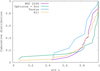 |
Fig. 1 Cumulative distribution of the sin i of observed dippers in three star-forming regions: NGC 2264 (purple line), ρ Oph + Upper Sco (green line) and Taurus (blue line). Also the total cumulative distribution (all) is shown as a yellow line. |
3 Description of the dusty funnel flow model
The paradigm explaining the few day periodicity of dippers is based on the explanation of the lc for the prototypical object AA Tau. The physical mechanism proposed by Bouvier et al. (1999) and used by many subsequent studies is that a dusty warp at the base of the magnetospheric stream periodically occults a section of the stellar surface. This phenomenon accounts for dipper lcs in high-inc systems. However, there exists a subsample of low-inc dippers that cannot be easily explained by this process. We propose here an alternative model to explain low-inclination dippers, namely dusty accreting funnel flows.
The main source of emission in the optical is the star. Periodic dips in the optical lc on a timescale of a few days can be interpreted as dusty structures located at the inner disk edge blocking part of the stellar radiation. The interpretation of the AA Tau lc (Bouvier et al. 1999) is based on this mechanism, where the occulting structure is a warp at the base of the mag-netospheric stream connecting the dusty disk and the star. This geometrical model is used in McGinnis et al. (2015) and Nagel & Bouvier (2020) to interpret a set of variable objects in the star-forming region NGC 2264. Bouvier et al. (1999); McGinnis et al. (2015) and others consider an optically thick warp that completely blocks some fraction of the stellar surface. Instead, Nagel & Bouvier (2020) compute the extinction component due to an evaporating dusty stream located between the disk and a hot spot formed in the stellar surface. The spot radiates the energy dissipated in a shock as the free-falling material in the stream hits the stellar surface. Dust survival within the accretion stream is relevant to interpret lcs of objects seen at a lower inclination than the high inclination required by the disk warp model. An argument in favor of this alternative or complementary mechanism is the existence of several objects with low inclination that display dipper lcs.
The physical model we develop to generate synthetic lcs is the partial occultation of the stellar surface by dust in the mag-netospheric streams. The streams result from material accreted from the disk that travels towards the magnetic poles at the stellar surface along the stellar magnetic field (B★)-lines. We assume this scenario because a dominant dipolar configuration for B★ is common among YSOs (Gregory et al. 2010; Donati et al. 2011, 2020). The formation of these structures occurs in a stable state corresponding to a mass accretion rate below some critical value (Kulkarni & Romanova 2009) while the signature of the unstable state is the formation of “tongues” of material around the equatorial plane, penetrating the B★-lines (Kulkarni & Romanova 2008). We assume a stable state where the rotation of the star and comoving magnetosphere periodically modulates the visibility of the accretion stream attached to the magnetic pole in the upper hemisphere, as seen by the observer. The effect is a dip periodically appearing in the optical light curve due to the extinction of the dusty funnel flow as it crosses the line of sight. The amplitude of the dip is strongly related to the geometry and the amount of dust around the star.
Li et al. (2022) present a model for the formation of planetesimals very close to the star by dust coagulation and fragmentation. The distribution of grain sizes delivered at the base of the accretion stream depends on these physical processes. We assume that small grains easily follow the fluid but large grains are not dragged by the gas. The critical size (rcrit) below which the grains are dragged away is calculated by equating the drag force with the vertical stellar gravity. Li et al. (2022) found that
 (1)
(1)
where the scale height of the disk H = cs/ΩK, ΩK is the keplerian angular velocity in the disk,  is the sound velocity with γ = 7/5 as the adiabatic index, K is the Boltzmann constant, m = 2.34 mp is the mean molecular weight with mp the proton mass, and T is the temperature. The average material density of silicate grains is ρ = 2.3 g cm−3, and ρs is the gas density at the disk launching height of the funnel flow. The value of rcrit is taken as the maximum size of the grains at the base of the stream in the models presented in Sect. 4.3. From this initial value, the size decreases as the particles evaporate during their approach to the star.
The gas density is related to the mass accretion rate Ṁ through the equations,
 (2)
(2)
where  is the rate at which material characterized with a surface density feeds the stream, and the factor of 2 in Eq. (2) means that the disk loses material toward the magnetic poles at both the upper and lower hemispheres. We assume that the width of the ring participating in this process is dR/R ~ 0.03 (Li et al. 2022).
The formation of the streams occurs where the disk is truncated by the stellar magnetic field (Königl 2011), which is given by:
 (3)
(3)
where B★ is the equatorial value of the dipolar component of the magnetic field at the stellar surface. The hydrodynamical interaction of the disk and the star through the magnetic field locates RT very close to the corotation radius Rco given by:
 (4)
(4)
where Prot is the rotational period of the star. We assume RT = Rco such that Ṁ can be extracted from
 (5)
(5)
The presence of dust at the inner edge of the disk is an unavoidable requirement because the high opacity of the grains is by far the largest contributor to the stellar extinction. For dippers, the estimate of the dust temperature (Td) at this location is below the evaporation temperature (Tevap) associated to the typical range of densities in this region. The dust temperature is calculated as in Nagel & Bouvier (2020) assuming an optically thin environment with heating from the stellar radiation.
The physical characteristics of the stream changes as the dust moves towards the star, and the stream can be divided in three regions: a non-evaporating layer defined by Td < Tevap, a dynamically evaporating layer with Td > Tevap, and an inner dust-free region. The density in the stream is defined by the amount of material falling to the star, assuming that the material follows the B★-lines. We use the accretion model of Hartmann et al. (1994) for a dipolar magnetic structure, which is consistent with magnetic surface maps of young accreting stars (Donati et al. 2011, 2020; Gregory et al. 2012). Because, Tevap weakly depends on density, the boundaries of the three regions strongly depend on the value of Td. Hartmann et al. (1994) assumes that Alfven waves formed at the hot spot are dissipated along the stream and heat the material to temperatures larger than 6000 K for most of the magnetosphere, steeply decreasing with radius close to RT. At these temperatures, the rate of evaporation, that is how fast the grain size decreases, is so large that the dust instantaneously dissipates. In the model presented below, we assume that Td results from an equilibrium between the absorbed stellar radiation and the emission by the grains in an optically thin environment, corresponding to weakly extincted YSOs.
Models of pre-main sequence accreting stars from Baraffe et al. (2017; see text) used to produce the synthetic lcs.
4 Synthetic dipper light curves simulating a star-forming region
4.1 The accreting stellar models
Nagel & Bouvier (2020) presented a model using a dusty magnetosphere as the occulting structure to explain the periodically extincted lc of the dipper V715 Persei. We aim here at exploring a wider parameter space in order to produce a full sample of synthetic light curves for young stellar objects covering a stellar mass range consistent with low-mass stars in star-forming regions. We thus define a sample of low-mass stars from Baraffe et al. (2017) pre-main sequence models of accreting stars, where the stellar parameters for each model are attached to a single value of Ṁ. Baraffe et al. (2017) self-consistent evolutionary models of accreting objects couple numerical hydrodynamics simulations of collapsing pre-stellar cores and stellar evolution models. They analyze two scenarios: the cold accretion model where all the accretion energy is radiated away and the hybrid accretion model in which some of the accretion energy is absorbed by the protostar. We focus on the hybrid model because we expect that some of the energy should be absorbed by the forming star. We support this choice with the fact that this model is able to explain the luminosity dispersion of young stellar objects in the Collinder 69 and the Orion Nebula clusters (Jensen & Haugbolle 2018). A set of 30 models are provided for accreting stars in the mass range from 0.06 to 1.69 M⊙ with values of Ṁ at an age of 2 Myr that are consistent with a stable state in the hydrodynamical simulations of Kulkarni & Romanova (2009). The Baraffe et al. (2017)’s models are also consistent with the estimate of lo𝑔(Ṁ) (−9 and −7.5) for a subset of dippers in the sample presented by Roggero et al. (2021). The stellar parameters combined with the value of M determine B★ through Eq. (5). We estimate B★ for the hybrid model sample at 2 Myr and further limit the sample to the 16 models within the mass range from 0.17 to 1.07 M⊙ that yield B★ ≤ 2 kG in order to be consistent with observations (Donati et al. 2011, 2020). Table 1 lists the parameters associated to each stellar model as well as B★ as derived from Eq. (5) and the threshold value of Ṁ such that Ṁ < Ṁerit corresponds to a stable accretion regime according to Kulkarni & Romanova (2008).
The dust abundance at the base of the stream defines the range of amplitudes of the synthetic models and we assume a typical gas-to-dust ratio ζd = 0.01 (Pollack 1994). The stellar rotational period (Prot) of young accreting stars ranges between 2 and 10 days with little dependence on stellar mass above 0.2 M⊙ (Rebull et al. 2018). We fix Prot at 8 days in the set of lcs presented below and explore shorter periods in Appendix B. For very low mass objects (M★ ≤ 0.2 M⊙), there is a correlation between M★ and Prot (Rebull et al. 2018, 2020, 2022). Among the 16 stellar models considered here, only two have such low masses. We explore the effect of shorter periods for lower mass objects in Appendix C and conclude that the main features in the distribution of lc amplitudes do not change.
With this set of accreting stellar models, the inclination remains the main parameter that drives the lc amplitude and the frequency occurrence of dippers, two quantities that can be directly compared to observations (see Sect. 2). We thus produce 80 synthetic lcs from the 16 models in Table 1, each one seen at five inclinations: i = 15, 30, 45, 60, 75°. These values are taken as typical for the last five bins of Table A.1. We do not consider very low values since all the dust is evaporated along the line of sight towards the star nor very large values as the optically thick part of the disk would completely occults the star, such that 15 < i < 75°.
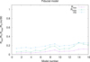 |
Fig. 2 Boundaries of the evaporating layer: (Rmin plus signs connected in purple and Rmax, crosses connected in green) for Case A (fiducial case). We present the 16 stars of the hybrid model at 2 Myr by Baraffe et al. (2017). The dust is not evaporating where R > Rmax and the dust-free region is located at R < Rmin. Also we present an estimate of the lower threshold of inc where we expect models producing dips for each of the stars in the sample. |
4.2 An optically thick funnel flow?
Using the models described above, we can now derive the radial boundaries of the dynamically evaporating dusty layer that determines the range of inclination over which the dipper phenomenon can be detected. The evaporation rate depends on Td, as mentioned in Sect. 3, which is calculated as in Nagel & Bouvier (2020) assuming heating by the stellar radiation in an optically thin environment.
In order to quantify this process, we present in Fig. 2 the radii associated to the boundaries of the evaporating layer for all the objects in the sample. We refer to this model as the fiducial case, Case A, where the dust temperature results from stellar irradiation alone. We follow a streamline starting at RT in the midplane of the disk to identify Rmax, the radius where the grains begin to evaporate and Rmin the radius where they complete this process. We assume the evaporation model of Xu et al. (2018) as described and implemented in Nagel & Bouvier (2020). The evaporation process starts where the saturation pressure (Psat) is larger than the gas pressure (Pg) and terminates where the opposite inequality holds. Psat depends on Td while Pg depends on the density of the gas in the stream which is connected to the density in the disk, in turn related to Ṁ. The value of Td where the equality holds corresponds to Tevap. For example, in Case A and model 1, Tevap = 2092 K and for model 9, Tevap = 1965 K.
Following this scheme we can estimate a lower threshold for inclination above which dipper light curves may be expected (see Fig. 2). The threshold value corresponds to the inclination of the line of sight connecting the lower part of the projected stellar surface (i.e. where the star starts to be occulted) and Rmin. The evaporating layer does not intersect the lines of sight inclined below this threshold, such that in this case the stellar extinction is not relevant. The radial extent of the layer changes according to the object’s parameters. The layer has a tendency to move toward larger radii when M★ increases. For each object, the values associated to Rmin and Rmax not only depend on the stellar parameters but also on the disk parameters, mainly Ṁ, because Tevap depends on the density. For this reason, Rmin and Rmax do not show monotonic behavior in terms of M★. The radial extent of the layer (Rmax – Rmin) changes between 0.023 and 0.14 RT. Note that the inclination threshold decreases when Rmin decreases and this tendency of Rmin is found if M★ decreases. From this we can conclude that low luminosity objects are prone to behave as low-inclined dippers.
In Sect. 3 we mention that the dust temperature, Td, estimated using the stellar heating can be underestimated because there is energy available coming from Alfven waves formed in the hotspot at the tip of the magnetospheric stream (Hartmann et al. 1994; Tessore et al. 2023). In order to analyze the effect of a higher dust temperature, we ran additional sets of models with an arbitrary increase of Td by a factor of 1.2 (Case B), 1.4 (Case C), and 1.6 (Case D). These are illustrated in Figs. 3,4, and 5, respectively. The behavior of Rmin and Rmax as Td increases can be seen in the sequence of cases starting with Case A as reference, followed by Cases B, C, and D, respectively. Figures 3–5 shows that the evaporating layer moves to larger radii as the temperatures increases compared to Fig. 2. From this we can conclude that the lower threshold of inclination to produce synthetic dippers increases when Td increases. The frequency occurrence of synthetic dippers in term of inclination for the various cases is presented in Sect. 4.3.
The main parameter defining the location of the evaporating layer is the radial profile of Td. As an example, we show the dust temperature profile within the funnel flow for stellar Model 1 and Model 9 in Fig. 6. Model 1 represents the star with the lowest luminosity; the case with the largest dust survival chances. The second model is a star with parameters closest to the typical star used in Tessore et al. (2023) (M★ = 0.5M⊙, R★ = 2 R⊙, T★ = 4000 K) to do the analysis of line emission in the magnetosphere. The largest value of Td is around 2300 K, i.e., only slightly larger than the evaporation temperature, Tevap ~ 1500–2000 K, and in this case the dust is not completely evaporated. For a short time span the dust can survive at a temperature larger than Tevap. The free fall time scale (tff) is around 10 h and according to the evaporation model used here, the evaporation occurs within this time span.
In Model 1, the dust reaches very close to the star, and this radius increases as the heating increases as can be seen in Fig. 6. The dust in Model 9 compared to Model 1 survives only at larger distances. This clearly illustrates that a low-inclination dipper can be produced only for low-luminosity objects.
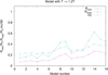 |
Fig. 3 Boundaries of the evaporating layer as in Fig. 2 but each model is recalculated with an increment of the temperature by a factor of 1.2, Case B. |
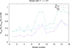 |
Fig. 4 Boundaries of the evaporating layer as in Fig. 2 but each model is recalculated with an increment of the temperature by a factor of 1.4, Case C. |
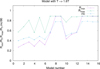 |
Fig. 5 Boundaries of the evaporating layer as in Fig. 2 but each model is recalculated with an increment of the temperature by a factor of 1.6, Case D. |
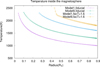 |
Fig. 6 Radial profile of the dust temperature Td in the accretion stream for the stellar Model 1 (lowest M★) and Model 9 (M★ = 0.534 M⊙) for Case A and D (see text). |
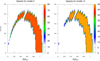 |
Fig. 7 Grain opacity multiplied by their abundance along the accretion stream is shown for the stellar Model 2 with M★ = 0.178 M⊙ and Model 14 with M★ = 0.832 M⊙. The color scale represent the opacity in units of cm2 g−1. |
4.3 The distribution of synthetic dipper light curve amplitudes
In Sect. 4.2, we described the size of the evaporating layer for the members of the sample. In order to complete the picture, we need to compute the opacity and abundance of the grains being evaporated. The largest size of the grains before the evaporation is given by rcrit (see Sect. 3). The grain population is integrated along all lines of sight intersecting the star to calculate the lc amplitude. We use the code presented in Nagel & Bouvier (2020) with a magnetic obliquity of 5° to derive the lcs amplitudes. We choose a lower mass (M★ = 0.178 M⊙) and a larger mass object (M★, = 0.832 M⊙) from the sample to illustrate in Fig. 7 the grain opacity multiplied by their abundance along the stream. A 2D cut along the accreting structure allows us to identify the differences in extinction in terms of the inclination, for two objects with different luminosity. A larger luminosity increases the evaporation such that the opacity increases due to grains with smaller sizes, while the abundance decreases, resulting in an overall reduction of the total extinction.
The amplitudes obtained for the 16 objects of the hybrid sample at 2 Myr (Baraffe et al. 2017) for Case A is presented in Fig. 8 for six values of inclination. At the lowest inclination (inc = 15°) the light curve amplitudes are well above the observational detection threshold (~0.05 mag, Roggero et al. 2021). The reason is that the contribution of the evaporation is not enough to counteract the contribution of the opacity increment due to the smaller grain sizes. Besides, the larger amplitude increases from Ampmax ~ 1.5 mag at inc = 15° to Ampmax ~ 7.8 mag at inc = 75°. The distribution of amplitudes in the sample of dippers in Taurus (Ampmax = 1.30 mag, Roggero et al. 2021) is well below the values associated to Case A. From this particular case, we can argue that in order to fit the observations we require an additional heating mechanism, as the dissipation of Alfvén waves coming from the hot spot as mentioned in Sect. 4.2.
The effect of an increment in the dust temperature is presented in Figs. 9–11 where we present the stellar models in Table 1 for Cases B, C, and D, respectively. The larger heating in Case B (see Fig. 9) results in a general decrement in the amplitudes. Also, the number of objects with detectable amplitudes at lower inc decreases. This means that the additional heating is able to remove all the dust close to the star for many cases. This behavior is further enhanced in Case C (see Fig. 9) where the larger heating rate decreases the number of synthetic dippers at low inc as well as the photometric amplitudes. The largest amplitude (Ampmax) at inc = 15/75° is 1.0/7.8 mag in Case B and 0.1/6.8 mag in Case C. The mean amplitudes (Ampmean) for all the models are 1.9 mag and 2.0 mag for Cases B and C, respectively. These values can be compared with the sample of dippers in NGC 2264 (McGinnis et al. 2015) and the sample in Taurus (Roggero et al. 2021). In NGC 2264, Ampmax ~ 1.0 mag and Ampmean ~ 0.5 mag and in Taurus, Ampmax = 1.30 mag and Ampmean = 0.41 mag. Neither Case B nor C are able to fit to the observed samples. For Case D, there are no dippers at inc = 15° and inc = 30°, thus, Ampmax = 0.0/5.9 mag at inc = 15/75°. for all the Cases, at inc = 75°, the value of Ampmax corresponds to a star being completely occulted. Note that the synthetic models (see Table 1) assumes that the sample is composed of one star for each mass. For a fair analysis, we should take into account that in a real star-forming region, there are a larger number of stars as the mass decreases. This will be included in a future paper about the interpretation of lcs using this mechanism in different star-forming regions.
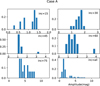 |
Fig. 8 Case A distribution of the light curve amplitudes for the stellar sample. The assumed system’s inclination is indicated in each panel. |
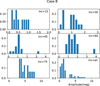 |
Fig. 9 Case B distribution of the light curve amplitudes for the stellar sample, as in Fig. 8 but with a factor 1.2 increment of the dust temperature. |
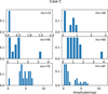 |
Fig. 10 Case C distribution of the light curve amplitudes for the stellar sample, as in Fig. 8 but with a factor 1.4 increment of the dust temperature. |
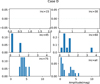 |
Fig. 11 Case D distribution of the light curve amplitudes for the stellar sample, as in Fig. 8 but with a factor 1.6 increment of the dust temperature. |
Fraction of expected dippers with an inclination larger than the inclination threshold inc0 for Cases A, B, C, and D.
4.4 The frequency occurrence of synthetic dippers
In the following we quantitatively compare the frequency occurrence of synthetic dippers with that of observed dippers as a function of inclination, using the observed samples with inclination estimates (see Table A.1). According to the physical model, there are not dippers in the first bin of inclination. However, it is important to include the value of zero dippers in this bin to estimate the fraction of dippers in Table 2. For the last five bins, the number of observed dippers and its fraction with respect to the total number of CTTSs in these bins are: 0 (0%), 3 (5.3%), 9 (15.8%), 16 (28%), 29 (50.9%). The same set of numbers for the synthetic sample are: Case A: 16 (20%), 16 (20%), 16 (20%), 16 (20%), 16 (20%); Case B: 10 (13.7%), 15 (20.6%), 16 (21.9%), 16 (21.9%), 16 (21.9%); Case C: 3 (5.9%), 7 (13.7%), 10 (19.6%), 15 (29.4%), 16 (31.4%), and Case D: 0 (0%), 0 (0%), 3 (13%), 10 (43.5%), 10 (43.5%), respectively. This indicates that we require to increase the temperature due to shock heating by a factor around 1.6 compared to stellar irradiation heating to get a set of dipper fractions consistent with the observed sample. A larger sample of young stellar objects with estimated inclinations and a larger synthetic sample of objects consistent with the stellar mass distribution of star-forming regions would be needed to strengthen this analysis.
In the previous calculations, we assumed that every low-luminosity CTTS possess a dusty magnetospheric stream and that the sample of stars used for the models is a reasonable representation of a star-forming region. We also assumed that the five values of inclination used to run the models are representative of the corresponding inclination bins used to characterize the distribution of observed dippers in Table A.1. We can therefore proceed to extract the fraction of dippers expected for an inclination higher than a given inclination threshold, inc0. The results are summarized in Table 2. According to Table 2, our best fit model Case D predicts a total fraction of dippers of 23.9%, assuming a random orientation of disk bearing stars in a particular star-forming region. This value should be compared with the fraction of dippers observed in various star-forming regions: Upper Sco (21.8%, Hedges et al. 2018), NGC 2264 (21.6%, Cody et al. 2014) and ρ Ophiuchus (20.1%, Hedges et al. 2018). Our current modeling suggests that Case D is the most relevant compared to observations. This comparison could be improved by including the fact that the number of stars to be considered in each mass bin should be consistent with the stellar mass function of star-forming regions. We leave a detailed tuning of other parameters, such as ζd, Prot among others, and a more thorough statistical fit of the observed samples to a following paper.
McGinnis et al. (2015) estimated that an inner disk warp is able to occult a section of the stellar surface when the system’s inclination ranges from 59 and 73°. For our Case D models, dippers occur at an inclination as low as 45°, and at even lower inclinations for Cases A, B, and C. This result is highly relevant when interpreting the observed lcs for systems exhibiting a large range of inclinations.
Finally, we note that for Case D there exists a dust free region for all the models inside a radius ~0.27 RT, as shown in Fig. 5. For a similar magnetospheric accretion model, assuming a star with a magnetic obliquity of 5°, Tessore et al. (2023) locates the Brγ emission inside a radius of 0.9 RT. The models of Tessore et al. (2023) assume a temperature profile for the accretion stream scaled to Tmax, the largest temperature in the funnel flow. Whether the dust temperature profile we derived to account for the fraction of dippers in star-forming region is consistent with the temperature profile of the gas in the funnel flow required to account for the Brγ line emission remains to be seen. The coupling between these two type of models is beyond the scope of this paper.
5 Conclusions
We presented a model where we assume that the dust located within the magnetospheric accretion stream periodically appearing along the line of sight toward the star is responsible for producing dips in the optical lcs of dippers. We used the stellar parameters of accreting pre-main sequence stellar models (Baraffe et al. 2017) to model the dynamical dust evaporation process along the magnetospheric accretion stream and derive the distribution of photometric amplitudes for dippers, for a range of system inclinations and assuming different heating rates for the dust grains. For a synthetic sample of low-mass stars consistent with accreting evolutionary tracks, we find that there is dust at the start of the accretion stream that can survive over some radial distance as it travels toward the star.
Our best fit model suggests a dust heating rate larger by a factor of about 1.6 than that produced by stellar irradiation alone. It predicts a fraction of dippers as a function of inclination consistent with observations. Notably, this model predicts the dipper phenomenon may occur for inclinations as low as 45°, while the inner disk warp model for dippers requires an inclination larger than 59°. The dusty funnel flow model also yields an overall fraction of dippers of order of 24% in star-forming regions, which bodes well with observations.
We will expand this study in a forthcoming paper by considering larger synthetic stellar samples whose mass distribution obeys that of star-forming regions and by exploring the impact of model parameters, such as the gas-to-dust ratio and the distribution of stellar rotational periods, on the statistical results.
Acknowledgements
E. Nagel acknowledges the support of the University of Guanajuato where this article was written. This project has received funding from the European Research Council (ERC) under the European Union’s Horizon 2020 research and innovation programme (Grant Agreement no. 742095; SPIDI: Star-Planets-Inner Disk-Interactions, https://www.spidi-eu.org).
Appendix A Additional table
Estimates of sin i for dippers in different stellar forming regions. We include the cumulative distribution for three different regions (CD) and the total cumulative distribution (TCD). Refs: (1) McGinnis et al. (2015) (2) Stauffer et al. (2015) (3) Barenfeld et al. (2017) (4) Ansdell et al. (2016a) (5) Ansdell et al. (2016b) (6) Roggero et al. (2021) (7) Rodriguez et al. (2017)
Appendix B The distribution of optical light curve amplitudes for stellar objects with Prot = 5 and 3d
For the analysis presented in the main text of this paper, we assumed Prot = 8d, which we take as a typical value for the rotational period of accreting young stars. This stands for solar-type stars (e.g. AA Tau), but lower mass stars tend to rotate faster in Taurus (Rebull et al. 2020) and other regions (Rebull et al. 2018, 2022). For the synthetic sample of objects used, Rco is distributed between 7 and 11R★. Because, Rco is proportional to  , Rco ranges from 5.31 to 7.96R★ for Prot = 5d, and from 3.78 to 5.67R★ for Prot = 3d.
The remaining parameters are the same as in the models in Sect. 4.3. For Prot = 3d, the distribution of the light curve amplitudes is presented in Fig.B1 for Case A (https://doi.org/10.5281/zenodo.12193027), in Fig.B2 for Case B (https://doi.org/10.5281/zenodo.12193115), in Fig. B3 for Case C (https://doi.org/10.5281/zenodo.12193135), and in Fig.B4 for Case D (https://doi.org/10.5281/zenodo.12193154). For Prot = 5d, the distribution of the amplitudes is presented in Fig.B5 for Case A (https://doi.org/10.5281/zenodo.12207247), in Fig. B6 for Case B (https://doi.org/10.5281/zenodo.12207274), in Fig. B7 for Case C (https://doi.org/10.5281/zenodo.12207284) and in Fig. B8 for Case D (https://doi.org/10.5281/zenodo.12207296). Each figure contains six histograms with the assumed system’s inclination indicated in each panel.
These models represent systems with the dusty stream being located closer to the star compared to the models that assume Prot=8d, whose distribution of amplitudes is shown in Figs. 8, 9, 10 and 11. A comparison between the different models indicates that the number of dippers decreases as Prot decreases. The extreme is Case D with Prot = 3d where the only two dippers are seen at inc = 75°.
The fraction of dippers for an inclination larger than a given threshold inc0 is listed for Cases A, B, C, and D is listed in Table B.2 for Prot = 3d and in Table B.1 for Prot = 5d. These values are notoriously lower than the values shown in Table 2 for Prot = 8d, a result consistent with the missing dippers due to accretion streams being closer to the star, thus having higher temperatures.
Fraction of dippers above the inclination threshold inc0 is listed for Cases A, B, C, and D, assuming Prot = 5d.
Fraction of dippers above the inclination threshold inc0 is listed for Cases A, B, C, and D, assuming Prot = 3d.
Appendix C The distribution of optical light curve amplitudes for stellar objects with Prot = 3d and a shorter Prot for very low mass objects
Prot measurements reported from surveys in Upper Scorpius (8 Myr) (Rebull et al. 2018), Taurus (3 Myr) (Rebull et al. 2020) and Upper Centaurus Lupus (16 Myr) with Lower Centaurus-Crux (17 Myr) (Rebull et al. 2022) show that Prot is distributed with a large dispersion as a function of M★ but can be assumed uniform for objects with spectral type earlier than M4 (M★ ≥ 0.2M⊙, Rebull et al. (2018)), while for objects with a spectral type later than M4, Prot decreases with M★. From our observed sample of dippers with estimates of inc shown in Table A.1 we see that there are four objects in the samples of Ansdell et al. (2016a) and Ansdell et al. (2016b) and two in the sample of Roggero et al. (2021) that fall into the very low-mass category. From our synthetic models used in this work (see Table 1) only two models (models 1 and 2) belong to the same category. We therefore assigned a value for Prot for these two models using as a reference the fit obtained for the sample of stars in Upper Scorpius (Rebull et al. 2018) using (V – K)o as a proxy for M★. This results in Prot = 2.476d for Model 1 and Prot = 2.73d for Model 2. The resulting histograms of photometric amplitudes at all inclinations are shown in Fig. C1 (https://doi.org/10.5281/zenodo.12207306) for Cases A, B, C, and D. Compared to previous models with uniformly distributed Prot=3d, we conclude that changing Prot for models 1 and 2 produces minimal differences.
References
- Alencar, S. H. P., Teixeira, P. S., Guimarães, M. M., et al. 2010, A&A, 519, A88 [NASA ADS] [CrossRef] [EDP Sciences] [Google Scholar]
- Alencar, S. H. P., Bouvier, J., Donati, J.-F., et al. 2018, A&A, 620, A195 [NASA ADS] [CrossRef] [EDP Sciences] [Google Scholar]
- Ansdell, M., Gaidos, E., Rappaport, S. A., et al. 2016a, ApJ, 816, 69 [Google Scholar]
- Ansdell, M., Gaidos, E., Williams, J. P., et al. 2016b, MNRAS, 462, L101 [Google Scholar]
- Baraffe, I., Elbakyan, V. G., Vorobyov, E. I., & Chabrier, G. 2017, A&A, 597, A19 [NASA ADS] [CrossRef] [EDP Sciences] [Google Scholar]
- Barenfeld, S. A., Carpenter, J. M., Sargent, A. I., Isella, A., & Ricci, L. 2017, ApJ, 851, 85 [Google Scholar]
- Bodman, E. H. L., Quillen, A. C., Ansdell, M., et al. 2017, MNRAS, 470, 202 [Google Scholar]
- Bohn, A. J., Benisty, M., Perraut, K., et al. 2022, A&A, 658, A183 [NASA ADS] [CrossRef] [EDP Sciences] [Google Scholar]
- Bouvier, J., Chelli, A., Allain, S., et al. 1999, A&A, 349, 619 [NASA ADS] [Google Scholar]
- Bouvier, J., Alencar, S. H. P., Boutelier, T., et al. 2007, A&A, 463, 1017 [NASA ADS] [CrossRef] [EDP Sciences] [Google Scholar]
- Cody, A. M., & Hillenbrand, L. A. 2018, AJ, 156, 71 [Google Scholar]
- Cody, A. M., Stauffer, J., Baglin, A., et al. 2014, AJ, 147, 82 [Google Scholar]
- Cohen, R. E., Herbst, W., & Williams, E. C. 2004, AJ, 127, 1602 [NASA ADS] [CrossRef] [Google Scholar]
- Donati, J.-F., Bouvier, J., Walter, F. M., et al. 2011, MNRAS, 412, 2454 [Google Scholar]
- Donati, J.-F., Bouvier, J., Alencar, S. H. P., et al. 2020, MNRAS, 491, 5660 [NASA ADS] [CrossRef] [Google Scholar]
- Fonseca, N. N. J., Alencar, S. H. P., Bouvier, J., Favata, F., & Flaccomio, E. 2014, A&A, 567, A39 [NASA ADS] [CrossRef] [EDP Sciences] [Google Scholar]
- Gaige, Y. 1993, A&A, 269, 267 [NASA ADS] [Google Scholar]
- Gregory, S. G., Jardine, M., Gray, C. G., & Donati, J.-F. 2011, Rep. Prog. Phys., 73, 126901 [Google Scholar]
- Gregory, S. G., Donati, J.-F., Morin, J., et al. 2012, ApJ, 755, 97 [Google Scholar]
- Hartmann, L., Hewett, R., & Calvet, N. 1994, ApJ, 426, 669 [Google Scholar]
- Hedges, C., Hodgkin, S., & Kennedy, G. 2018, MNRAS, 476, 2968 [Google Scholar]
- Herbig, G. H. 1998, ApJ, 497, 736 [NASA ADS] [CrossRef] [Google Scholar]
- Jensen, S. S., & Haugbolle, T. 2018, MNRAS, 474, 1176 [NASA ADS] [CrossRef] [Google Scholar]
- Königl, A., Romanova, M. M., & Lovelace, R. V. E. 2011, MNRAS, 416, 757 [NASA ADS] [Google Scholar]
- Kulkarni, A. K., & Romanova, M. M. 2008, MNRAS, 386, 673 [Google Scholar]
- Kulkarni, A. K., & Romanova, M. M. 2009, MNRAS, 398, 701 [Google Scholar]
- Li, R., Chen, Y.-X, & Lin, D. N. C. 2022, MNRAS, 510, 5246 [NASA ADS] [CrossRef] [Google Scholar]
- McGinnis, P. T., Alencar, S. H. P., Guimaraes, M. M., et al. 2015, A&A, 577, A11 [NASA ADS] [CrossRef] [EDP Sciences] [Google Scholar]
- Morales-Calderón, M., Stauffer, J. R., Hillenbrand, L. A., et al. 2011, ApJ, 733, 50 [CrossRef] [Google Scholar]
- Nagel, E., & Bouvier, J. 2019, A&A, 625, A45 [NASA ADS] [CrossRef] [EDP Sciences] [Google Scholar]
- Nagel, E., & Bouvier, J. 2020, A&A, 643, A157 [EDP Sciences] [Google Scholar]
- Pecaut, M. J., & Mamajek, E. E. 2020, A&A, 643, A157 [NASA ADS] [CrossRef] [EDP Sciences] [Google Scholar]
- Pollack, J. B., Hollenbach, D., Beckwith, S., et al. 1994, ApJ, 421, 615 [Google Scholar]
- Rebull, L. M., Stauffer, J. R., Cody, A. M., et al. 2018, AJ, 155, 196 [Google Scholar]
- Rebull, L. M., Stauffer, J. R., Cody, A. M., et al. 2020, AJ, 159, 273 [Google Scholar]
- Rebull, L. M., Stauffer, J. R., Hillenbrand, L. A., et al. 2022, AJ, 164, 80 [NASA ADS] [CrossRef] [Google Scholar]
- Rodriguez, J. E., Ansdell, M., Oelkers, R. J., et al. 2017, ApJ, 848, 97 [Google Scholar]
- Roggero, N., Bouvier, J., Rebull, L. M., & Cody, A. M. 2021, A&A, 651, A44 [NASA ADS] [CrossRef] [EDP Sciences] [Google Scholar]
- Romanova, M. M., Ustyugova, G. V., Koldova, A. V., & Lovelace, R. V. E. 2013, MNRAS, 430, 699 [NASA ADS] [CrossRef] [Google Scholar]
- Sicilia-Aguilar, A., Manara, C. F., de Boer, J., et al. 2020, A&A, 633, A37 [NASA ADS] [CrossRef] [EDP Sciences] [Google Scholar]
- Stauffer, J., Cody, A. M., Baglin, A., et al. 2014, AJ, 147, 83 [Google Scholar]
- Stauffer, J., Cody, A. M., McGinnis, P., et al. 2015, AJ, 149, 130 [Google Scholar]
- Tessore, B., Soulain, A., Pantolmos, G., et al. 2023, A&A, 671, A129 [NASA ADS] [CrossRef] [EDP Sciences] [Google Scholar]
- Xu, S., Rappaport, S., van Lieshout, R., et al. 2018, MNRAS, 474, 4 [Google Scholar]
All Tables
Models of pre-main sequence accreting stars from Baraffe et al. (2017; see text) used to produce the synthetic lcs.
Fraction of expected dippers with an inclination larger than the inclination threshold inc0 for Cases A, B, C, and D.
Estimates of sin i for dippers in different stellar forming regions. We include the cumulative distribution for three different regions (CD) and the total cumulative distribution (TCD). Refs: (1) McGinnis et al. (2015) (2) Stauffer et al. (2015) (3) Barenfeld et al. (2017) (4) Ansdell et al. (2016a) (5) Ansdell et al. (2016b) (6) Roggero et al. (2021) (7) Rodriguez et al. (2017)
Fraction of dippers above the inclination threshold inc0 is listed for Cases A, B, C, and D, assuming Prot = 5d.
Fraction of dippers above the inclination threshold inc0 is listed for Cases A, B, C, and D, assuming Prot = 3d.
All Figures
|
Fig. 1 Cumulative distribution of the sin i of observed dippers in three star-forming regions: NGC 2264 (purple line), ρ Oph + Upper Sco (green line) and Taurus (blue line). Also the total cumulative distribution (all) is shown as a yellow line. |
| In the text | |
|
Fig. 2 Boundaries of the evaporating layer: (Rmin plus signs connected in purple and Rmax, crosses connected in green) for Case A (fiducial case). We present the 16 stars of the hybrid model at 2 Myr by Baraffe et al. (2017). The dust is not evaporating where R > Rmax and the dust-free region is located at R < Rmin. Also we present an estimate of the lower threshold of inc where we expect models producing dips for each of the stars in the sample. |
| In the text | |
|
Fig. 3 Boundaries of the evaporating layer as in Fig. 2 but each model is recalculated with an increment of the temperature by a factor of 1.2, Case B. |
| In the text | |
|
Fig. 4 Boundaries of the evaporating layer as in Fig. 2 but each model is recalculated with an increment of the temperature by a factor of 1.4, Case C. |
| In the text | |
|
Fig. 5 Boundaries of the evaporating layer as in Fig. 2 but each model is recalculated with an increment of the temperature by a factor of 1.6, Case D. |
| In the text | |
|
Fig. 6 Radial profile of the dust temperature Td in the accretion stream for the stellar Model 1 (lowest M★) and Model 9 (M★ = 0.534 M⊙) for Case A and D (see text). |
| In the text | |
|
Fig. 7 Grain opacity multiplied by their abundance along the accretion stream is shown for the stellar Model 2 with M★ = 0.178 M⊙ and Model 14 with M★ = 0.832 M⊙. The color scale represent the opacity in units of cm2 g−1. |
| In the text | |
|
Fig. 8 Case A distribution of the light curve amplitudes for the stellar sample. The assumed system’s inclination is indicated in each panel. |
| In the text | |
|
Fig. 9 Case B distribution of the light curve amplitudes for the stellar sample, as in Fig. 8 but with a factor 1.2 increment of the dust temperature. |
| In the text | |
|
Fig. 10 Case C distribution of the light curve amplitudes for the stellar sample, as in Fig. 8 but with a factor 1.4 increment of the dust temperature. |
| In the text | |
|
Fig. 11 Case D distribution of the light curve amplitudes for the stellar sample, as in Fig. 8 but with a factor 1.6 increment of the dust temperature. |
| In the text | |
Current usage metrics show cumulative count of Article Views (full-text article views including HTML views, PDF and ePub downloads, according to the available data) and Abstracts Views on Vision4Press platform.
Data correspond to usage on the plateform after 2015. The current usage metrics is available 48-96 hours after online publication and is updated daily on week days.
Initial download of the metrics may take a while.