| Issue |
A&A
Volume 687, July 2024
|
|
|---|---|---|
| Article Number | A186 | |
| Number of page(s) | 14 | |
| Section | Cosmology (including clusters of galaxies) | |
| DOI | https://doi.org/10.1051/0004-6361/202449267 | |
| Published online | 09 July 2024 | |
Resistively controlled primordial magnetic turbulence decay
1
Nordita, KTH Royal Institute of Technology and Stockholm University, Hannes Alfvéns väg 12, 10691 Stockholm, Sweden
e-mail: brandenb@nordita.org
2
The Oskar Klein Centre, Department of Astronomy, Stockholm University, AlbaNova, 10691 Stockholm, Sweden
3
McWilliams Center for Cosmology & Department of Physics, Carnegie Mellon University, 5000 Forbes Ave, Pittsburgh, PA 15213, USA
4
School of Natural Sciences and Medicine, Ilia State University, 3-5 Cholokashvili Avenue, 0194 Tbilisi, Georgia
5
Department of Astrophysics, American Museum of Natural History, 200 Central Park West, New York, NY 10024, USA
6
Astroparticules et Cosmologie, Université Paris Cité, CNRS, Astroparticule et Cosmologie, 75006 Paris, France
7
Laboratory of Astrophysics, École Polytechnique Fédérale de Lausanne, 1015 Lausanne, Switzerland
8
Dipartimento di Fisica e Astronomia, Università di Bologna, Via Gobetti 93/2, 40129 Bologna, Italy
9
INAF Istituto di Radioastronomia, Via P. Gobetti 101, 40129 Bologna, Italy
10
Hamburger Sternwarte, Universität Hamburg, Gojenbergsweg 112, 41029 Hamburg, Germany
Received:
18
January
2024
Accepted:
17
March
2024
Context. Magnetic fields generated in the early Universe undergo turbulent decay during the radiation-dominated era. The decay is governed by a decay exponent and a decay time. It has been argued that the latter is prolonged by magnetic reconnection, which depends on the microphysical resistivity and viscosity. Turbulence, on the other hand, is not usually expected to be sensitive to microphysical dissipation, which affects only very small scales.
Aims. We want to test and quantify the reconnection hypothesis in decaying hydromagnetic turbulence.
Methods. We performed high-resolution numerical simulations with zero net magnetic helicity using the PENCIL CODE with up to 20483 mesh points and relate the decay time to the Alfvén time for different resistivities and viscosities.
Results. The decay time is found to be longer than the Alfvén time by a factor that increases with increasing Lundquist number to the 1/4 power. The decay exponent is as expected from the conservation of the Hosking integral, but a timescale dependence on resistivity is unusual for developed turbulence and not found for hydrodynamic turbulence. In two dimensions, the Lundquist number dependence is shown to be leveling off above values of ≈25 000, independently of the value of the viscosity.
Conclusions. Our numerical results suggest that resistivity effects have been overestimated in earlier work. Instead of reconnection, it may be the magnetic helicity density in smaller patches that is responsible for the resistively slow decay. The leveling off at large Lundquist number cannot currently be confirmed in three dimensions.
Key words: early Universe
© The Authors 2024
 Open Access article, published by EDP Sciences, under the terms of the Creative Commons Attribution License (https://creativecommons.org/licenses/by/4.0), which permits unrestricted use, distribution, and reproduction in any medium, provided the original work is properly cited.
This article is published in open access under the Subscribe to Open model. Subscribe to A&A to support open access publication.
1. Introduction
Decaying turbulence played an important role in the early Universe during the radiation-dominated era, when the magnetic field is well coupled to the plasma. While turbulence speeds up the decay, it can also lead to a significant increase in the typical length scale, which could then be many times larger than the comoving horizon scale at the time of magnetic field generation (Brandenburg et al. 1996; Christensson et al. 2001; Banerjee & Jedamzik 2004). This is important because magnetogenesis processes during the electroweak era, when the age of the Universe was just a few picoseconds (Vachaspati 1991; Cheng & Olinto 1994; Baym et al. 1996), tend to produce magnetic fields of very small length scales of the order of 1 AU or less (in comoving units).
From the study of decaying hydrodynamic turbulence, it has been known for a long time that turbulent energy density and length scale evolve as power laws (Batchelor 1953; Saffman 1967). The exponents depend on the physics of the decay, specifically on the possibility of a conserved quantity that governs the decay, for example magnetic helicity in the hydromagnetic case (Hatori 1984; Biskamp & Müller 1999). The endpoints of the evolution, however, depend on the relevant timescale, which is traditionally taken to be just the turnover or, in the magnetic case that we consider here, the Alfvén time (Banerjee & Jedamzik 2004). More recently, Hosking & Schekochihin (2023) argued that the turnover time should be replaced by the reconnection time, which could be significantly longer (up to 105.5 times). This would result in an endpoint where the magnetic field strength is greater and the turbulent length scale smaller than otherwise, when the decay time is just the Alfvén time.
One of the hallmarks of turbulence is that its large-scale properties are nearly independent of viscosity and resistivity, which act predominantly on the smallest scales of the system. On the other hand, magnetic reconnection is a process that could potentially limit the speed of the inverse cascade. This idea has been invoked by Hosking & Schekochihin (2023) to explain a premature termination of the decay process by the time of recombination of the Universe, when its age was about 400 000 years.
The purpose of our paper is to analyze numerical simulations with respect to their decay times at different values of resistivity. In Sect. 2 we discuss the decay time and its relation to other quantities. In Sect. 3 we present our numerical simulation setup and show the results for a resistivity-dependent decay in Sect. 4. We then make a comparison with a purely hydrodynamic decay in Sect. 5 and with the two-dimensional (2D) hydromagnetic case in Sect. 6, before concluding in Sect. 8. In Appendix A we provide a historical note on the anastrophy, i.e., the mean squared magnetic vector potential, and in Appendix B, we show detailed convergence tests for some of our 2D results.
2. Decay and turnover times
In the following we focus on the decay of magnetic field. Magnetically dominated turbulence is characterized by the turbulent magnetic energy density ℰM and the magnetic integral scale ξM. Both ℰM(t) and ξM(t) can be defined in terms of the magnetic energy spectrum EM(k, t), such that ℰM = ∫EM dk and ξM = ∫k−1EM dk/ℰM. In decaying turbulence, both quantities depend algebraically rather than exponentially on time. Therefore, the decay is primarily characterized by power laws,

rather than by exponential laws of the type ℰM ∝ e−t/τ. The algebraic decay is mainly a consequence of nonlinearity. On the other hand, in decaying hydromagnetic turbulence with significant cross-helicity, for example, the nonlinearity in the induction equation is reduced and then the decay is indeed no longer algebraic, but closer to exponential (see Brandenburg & Oughton 2018).
An obvious difference between algebraic and exponential decays is that in the former ℰM(t) is characterized by the nondimensional quantity p, while in the latter it is characterized by the dimensionful quantity τ. Following Hosking & Schekochihin (2023), a decay time τ can also be defined for an algebraic decay and is then given by
In the present case of a power-law decay, this value of τ = τ(t) is time-dependent and can be related to the instantaneous decay exponent

through τ = t/p(t) (i.e., no new parameter emerges except for t itself). However, a useful way of incorporating new information is by relating τ to the Alfvén time τA = ξM/vA through
where CM is a nondimensional parameter, and vA is the Alfvén velocity, which is related to the magnetic energy density through  , where ρ is the density, μ0 the vacuum permeability, and Brms the root mean square (rms) magnetic field.
As was noted by Hosking & Schekochihin (2023), Eq. (4) can be used to define the endpoints of the evolutionary tracks in a diagram of Brms versus ξM or, equivalently, vA versus ξM (i.e., vA = vA(ξ)). They also noted that the location of these endpoints is sensitive to whether or not CM depends on the resistivity of the plasma. If it does depend on the resistivity, this could be ascribed to the effects of magnetic reconnection, which might slow down the turbulent decay.
Magnetic reconnection refers to a change in magnetic field line connectivity that is subject to topological constraints. A standard example is x-point reconnection (see, e.g., Craig & McClymont 1991; Craig et al. 2005), which becomes slower as the x-point gets degenerated into an extremely elongated structure (Sweet 1958; Parker 1957; see Liu et al. 2022 for a review). It is usually believed that in the presence of turbulence, such structures break up into progressively smaller ones, which makes reconnection eventually fast (i.e., independent of the microphysical resistivity; Galsgaard & Nordlund 1996; Lazarian & Vishniac 1999; Comisso & Sironi 2019). However, whether this would also imply that τ becomes independent of the resistivity remains an unclear issue. For example, Galsgaard & Nordlund (1996) found that resistive heating becomes independent of the value of the resistivity. Another question concerns the speed at which magnetic flux can be processed through a current sheet (Kowal et al. 2009; Loureiro et al. 2012). Also of interest is the timescale on which the topology of the magnetic field changes (Lazarian et al. 2020). These different timescales may not all address the value of CM that relates the decay time to the Alfvén time.
In magnetically dominated turbulence, the effect of the resistivity is quantified by the Lundquist number. For decaying turbulence, it is time-dependent and defined as

This quantity is similar to the magnetic Reynolds number if we replace vA by the rms velocity, urms. Here, however, the plasma is driven by the Lorentz force, so the Lundquist number is a more direct way of quantifying the resistivity than the magnetic Reynolds number. The Alfvénic Mach number is defined as MaA = urms/vA.
In addition to varying η, we also vary ν such that the magnetic Prandtl number PrM = ν/η is typically in the range 1 ≤ PrM ≤ 5. It is then also convenient to define the Lundquist number based on the reconnection outflow,
(see Hosking & Schekochihin 2023 for details).
3. Numerical simulations
We performed simulations of the compressible hydromagnetic equations for the magnetic vector potential A, the velocity u, and the logarithmic density lnρ in the presence of viscosity ν and magnetic diffusivity η:
![$$ \begin{aligned} \frac{ \mathrm{D}\boldsymbol{u}}{ \mathrm{D} t}&= \frac{1}{\rho }\left[\boldsymbol{J}\times \boldsymbol{B}+{\boldsymbol{\nabla }}\cdot (2\rho \nu \boldsymbol{\mathsf{S }})\right] -c_{\rm s}^2{\boldsymbol{\nabla }}\ln \rho , \end{aligned} $$](/articles/aa/full_html/2024/07/aa49267-24/aa49267-24-eq9.gif)
We used a random magnetic field as the initial condition, such that EM(k, 0) has a k4 subinertial range for k < kp (Durrer & Caprini 2003), and a k−2 inertial range for k > kp (Brandenburg et al. 2015). In all cases we chose kp/k1 = 60, where k1 = 2π/L is the smallest wavenumber in our cubic domain of size L3. In Eqs. (7) and (8), B = ∇ × A is the magnetic field, J = ∇ × B/μ0 is the current density, and Sij = (∂iuj + ∂jui)/2 − δij∇ ⋅ u/3 are the components of the rate-of-strain tensor S.
There is no magnetic helicity on average, but the fluctuations in the local magnetic helicity density h = A ⋅ B lead to a decay behavior where the correlation integral of h, which is also known as the Hosking integral, is conserved (Hosking & Schekochihin 2021; Schekochihin 2022; Zhou et al. 2022). We use the PENCIL CODE (Pencil Code Collaboration 2021), which has also been used for many earlier simulations of decaying hydromagnetic turbulence (Zhou et al. 2022; Brandenburg et al. 2023). All our simulations are in the magnetically dominated regime, because the velocity is just a consequence of and driven by the magnetic field.
Because the magnetic field is initially random, the resulting velocity is also random and it drives a forward turbulent cascade with kinetic and magnetic energy dissipation rates ϵK = ⟨2νρS2⟩ and ϵM = ⟨ημ0J2⟩. Their ratio scales with  (Brandenburg 2014; Galishnikova et al. 2022). If kp/k1 is large (we recall that we use the value 60), there is also an inverse cascade (Brandenburg et al. 2015). The inverse cascade was also found in the relativistic regime (Zrake 2014) and is now understood to be a consequence of the conservation of the Hosking integral (Hosking & Schekochihin 2021; Schekochihin 2022; Zhou et al. 2022). However, the role played by the Hosking integral is currently not universally accepted (Armua et al. 2023; Dwivedi et al. 2024). The lack of numerical support could be related to insufficiently large values of kp/k1.
We define the kinetic energy spectrum EK(k, t) analogously to EM(k, t), using the normalization  , where ρ0 = ⟨ρ⟩=const owing to mass conservation. In magnetically driven turbulence, ℰK is about one-tenth of
  , which seems to be surprisingly independent of the physical input parameters (Brandenburg et al. 2017).
In Table 1 we summarize the results of five simulations, Runs M0–M5, where we vary η and ν and also vary the number of mesh points, N3. We present some relevant output parameters that are defined below. They are all obtained from a statistically steady stretch of our time series data, and the error bars were calculated as the largest departure from any one-third of the time series. A visualization of the z components of B on the periphery of the computational domain for Run M1 is shown in Fig. 1. Figure 2 shows Jz in an xy plane together with a zoom-in on the lower left corner of the domain. The corresponding magnetic and kinetic energy spectra are shown in Fig. 3 for different times in units of [t]=(csk1)−1.
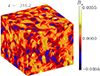 |
Fig. 1. Visualization of Bz on the periphery of the computational domain for Run M1, where PrM = 5. |
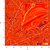 |
Fig. 2. Visualization of Jz at z = π along with a zoom-in on the lower left corner for Run M0, where PrM = 10, at t = 644. The value of ξM at that time is indicated by the length of the short white lines. |
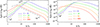 |
Fig. 3. Magnetic and kinetic energy spectra for Run M1 at different times. For large values of k there is a k−2 inertial range. The ∝k4 and ∝k2 slopes are indicated for reference. As elsewhere, time is in units of [t]=(csk1)−1. |
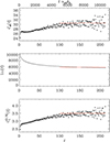 |
Fig. 4. Approach of CM(t), Lu(t), and |

Summary of magnetohydrodynamic simulations analyzed in this paper.
The EM(k, t)∝k−2 inertial range can be explained by weak turbulence scaling (Brandenburg et al. 2015), but it becomes a bit shallower near the dissipation subrange. This could follow from some kind of magnetic bottleneck effect associated with reconnection, analogously to the bottleneck effect in hydrodynamic turbulence (Falkovich 1994).
It should be noted that at late times, the subinertial range spectrum of EM(k, t) becomes shallower than the initial k4 slope. This is an artifact of poor scale separation (see Brandenburg et al. 2023 for related numerical evidence). On the other hand, a k2 subinertial range for EK(k, t) has been seen for some time (see Kahniashvili et al. 2013).
In our numerical simulations we use units such that cs = k1 = ρ0 = μ0 = 1. The resistivity, μ0η, is therefore the same as the magnetic diffusivity. Nevertheless, most of the results below are expressed in manifestly nondimensional form.
4. Resistivity-dependent decay
We now analyze a collection of runs similar to those of the recent works of Zhou et al. (2022) and Brandenburg et al. (2023), who considered different values of Lu and also included some runs with hyperviscosity and hyperresistivity, unlike what we present in the present work. At variance with those earlier papers, where the focus was always on the decay exponent p(t), here we focus on the evolution of the decay time, τ(t) = t/p(t).
4.1. Decay time
The goal is to determine the prefactor in the scaling relation τ ∝ ξM/vA. Therefore, we write
and determine

We emphasize here that each of the terms is time-dependent, including τ(t) = t/p(t), as already noted above. Interestingly, it turns out that the quantity CM(t) eventually settles around a plateau:
Here and in the following, when time-dependence is not indicated, we usually mean that the value is obtained as a suitable limit of the corresponding time-dependent function. In numerical simulations with finite domains, the limit t → ∞ needs to be evaluated with some care to prevent the final result from being contaminated by finite size effects. We do this by selecting a suitable time interval during which certain data combinations are approximately statistically stationary. We refer to these results as late-time limits.
In Fig. 4 we show that CM(t) and Lu(t) approach an approximately constant value toward the end of the run. Time is given both in units of [t]=(csk1)−1 and in initial Alfvén times, (vA0kp)−1, where  is the initial Alfvén velocity and ℰM0 the initial magnetic energy density. Allowing for the possibility of power-law scaling,
  , we also plot the prefactor
  for n = 1/4 in the last panel of Fig. 4 (see details below). Toward the end of the simulation, however, there is an increase in the fluctuations, which follows from the decrease in the magnetic energy.
As discussed below in more detail in connection with 2D simulations, current sheets are underresolved at early times, when ξM is small. As we now see from Fig. 4, this underestimates the resulting value of CM. However, for t > 100, CM(t) approaches a plateau, suggesting that the simulation now begins to be sufficiently well resolved, at least for the purpose of determining CM.
In Fig. 5 we show the dependence of CM on Lu and Luν. We see an approximate scaling ∝Lun with n = 1/4 for Lu < 6000 and a piecewise power-law scaling  , but with different prefactors for the runs with larger and smaller values of the viscosity. We note that for PrM ≫ 1 we have
  , which explains why the
  scaling is found to be compatible with being ∝Lu1/4. We also note, however, that for a higher viscosity, the line
  is shifted upward (toward larger values of CM). Owing to the more complicated combined dependence on ν and Luν, we continue to employ the simpler Lun scaling for the following discussion. It is worth noting that the exponent n = 1/4 is discussed in Uzdensky & Loureiro (2016) in connection with the fast growing mode of the tearing instability.
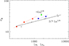 |
Fig. 5. Dependence of CM on Lu and Luν. An approximate scaling ∝Lu1/4 is found for Lu < 6000 and a piecewise power-law scaling |

If it is really true that CM is proportional to Lun, as found above, we can write  , and then determine
  as the late-time limit of
This is the formula that was used to compute  and to plot its time-dependence
  for n = 1/4 (see the last panel of Fig. 4). From Table 1 we find
  .
.
4.2. Evolution of ℰM(t) and ξM(t)
It is of interest to know whether the resistivity dependence of CM(t) is equally distributed among ξM and vA (or ℰM). Figure 6 shows that there are indeed systematic differences in the decay laws for different values of the resistivity, but the differences are small and easily overlooked.
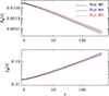 |
Fig. 6. Dependence of ℰM(t) and ξM(t) for three values of PrM. |
To examine the dependence of CM(t) on Lu, we write the decay laws for ξM(t) and ℰM(t) in a more detailed form than Eq. (1):

Here the coefficients ξM0 and ℰM0 just depend on the initial condition, and are thus not dependent on Lu, which means that the Lu-dependence can only enter through the coefficients τξ and τℰ. We can determine them as the limits of the time-dependent functions τξ(t) and τℰ(t), which are obtained by inverting Eqs. (14) and (15), and are given by
![$$ \begin{aligned} \tau _\xi (t)=\frac{t}{\left[{\xi _{\rm M}}(t)/{\xi _{\rm M0}}\right]^{1/q}-1}, \end{aligned} $$](/articles/aa/full_html/2024/07/aa49267-24/aa49267-24-eq35.gif)
![$$ \begin{aligned} \tau _{\mathcal{E} }(t)=\frac{t}{\left[{{\mathcal{E} }_{\rm M}}(t)/{{\mathcal{E} }_{\rm M0}}\right]^{-1/p}-1}. \end{aligned} $$](/articles/aa/full_html/2024/07/aa49267-24/aa49267-24-eq36.gif)
Figure 7 shows the evolution of τξ(t) and τℰ(t) for Runs M3–M5 with fixed and moderate viscosity.
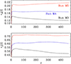 |
Fig. 7. Evolution of τℰ(t) and τξ(t) for three values of PrM with fixed and moderate viscosity. These times tend to be approximately constant at late times with values approximately consistent with those in Table 1. |
Using the late-time limits of Eqs. (14) and (15), and those of Eqs. (16) and (17), the equation for CM can now be decomposed in the form

such that Eq. (11) is obeyed. Here we can determine Cξ and Cℰ as the late-time limits of

In this connection, it it important to remember that for a self-similar evolution (Brandenburg & Kahniashvili 2017), which is here approximately satisfied (see Fig. 3), we have

so that CM = (t/p) vA/ξM is obeyed. For t ≫ τℰ, τξ, using again τ = τ(t) = t/p(t), we have

so that  . It is then natural to expect that both τξ and τℰ scale in the same way with Lu as CM itself. Equation (21) also allows us to compute the timescales τξ = p (CξξM0)1/q and τℰ = p (Cℰ/vA0)2/p.
In Fig. 8 we show the dependence of τξ and τℰ on Lu. While the two show a similar dependence, approximately ∝Lu1/4, we note that there is also possible evidence for a leveling off for larger values of Lu.
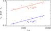 |
Fig. 8. Dependence of τξ and τℰ on Lu. The two show a similar dependence on Lu, approximately ∝Lu1/4, but there is possible evidence for a leveling off for larger values of Lu. |
5. Comparison with hydrodynamic decay
Hydrodynamic decay is characterized by the kinetic energy density  and the hydrodynamic integral scale ξK(t) = ∫k−1EK dk/ℰK. We define the instantaneous kinetic energy decay exponent pK(t) = − dlnℰK/dlnt and the decay time τK(t) = t/pK(t). We relate τK(t) to the turnover time urms/ξK through τK = CKξK/urms, and thus determine CK as the late-time limit of CK(t) = [t/pK(t)] urms(t)/ξK(t), which is defined analogously to Eq. (11).
Purely hydrodynamic simulations can be performed by just ignoring the magnetic field, or putting B = 0. In Table 2 we summarize such simulations for different values of ν, which is quantified by the Reynolds number: Re = urmsξK/ν. Figure 9 shows, for Re ≥ 100, that CK does not change much with Re. This was not expected. It also confirms that the prolonged decay time found in Sect. 4 is indeed a purely magnetic phenomenon. Whether or not the resistivity dependence in the magnetic case must be ascribed to reconnection remains an open question. As discussed in Sect. 2, magnetic reconnection refers to topologically constrained changes of magnetic field lines, but in the present case of a turbulent magnetic field there is no connection with the standard picture of reconnection. An obvious alternative candidate for explaining the resistively prolonged decay time may be related to magnetic helicity conservation in local patches, as described by the conservation of the Hosking integral. While this idea seems more plausible to us, it is not obvious how to distinguish reconnection from magnetic helicity conservation in patches. It is true that magnetic helicity would vanish in two dimensions, but in that case it should be replaced by the anastrophy (see Appendix A for a historical note on this word). One aspect that might be different between the concepts of reconnection and magnetic helicity conservation in patches could be the dependence on PrM. Our present results have not yet shown such a dependence, which might support the idea that the dependence on resistivity is related to magnetic helicity conservation in patches.
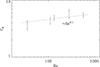 |
Fig. 9. Dependence of CK on Re. The line Re0.1 is shown for comparison, but the data are also nearly compatible with being independent of Re. |
6. Hydromagnetic decay in two dimensions
We now perform 2D simulations where  lies entirely in the xy plane (see Table 3 for a summary). Equation (7) then reduces to
which obeys conservation of anastrophy,  (Fyfe & Montgomery 1976; Pouquet 1978, 1993), and the magnetic helicity density vanishes pointwise, so the Hosking integral is then also zero. These simulations are different from the recent ones by Dwivedi et al. (2024), who performed 2.5D simulations. In their case, there was a magnetic field component out of the plane. The anastrophy was then not conserved and the Hosking integral was finite.
As we stated above, our present measurements of CM as a function of Lu cannot directly be compared with the reconnection rate determined by Loureiro et al. (2012), Comisso et al. (2015), or Comisso & Bhattacharjee (2016). In addition, it is not obvious how relevant a 2D simulation is in the present context because in 2D the anastrophy is conserved, while the Hosking integral is strictly vanishing.
In our present purely 2D simulations, values of Lu up to about 3 × 10⁵ have been reached. To allow for a longer nearly self-similar evolution, we used kp/k1 = 200 instead of 60. The simulation results give the prefactors in the scaling expected from anastrophy conservation as

where μ0 = ρ0 = 1 is used. We also see from Fig. 10 that the spectral peaks evolve underneath an envelope  .
.
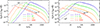 |
Fig. 10. Similar to Fig. 3, but for Run 2M1. The magnetic peaks lie underneath a kβ envelope with β = 1, as expected in the case of anastrophy conservation. |
Figure 11 shows magnetic and kinetic energy spectra for Run 2m2 with Lu = 1.8 × 10⁵ collapsed on top of each other by plotting  versus kξM(t) for β = 1. This plot suggests that the subinertial range scalings of EM(k, t) and EK(k, t) are proportional to k5 and k3, respectively. Thus, they are steeper than expected in 3D. This behavior is in some ways similar to the steepening observed for helical decaying magnetic fields (see Brandenburg & Kahniashvili 2017).
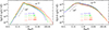 |
Fig. 11. Magnetic energy spectra (left) and kinetic energy spectra (right) for Run 2m2 with Lu = 1.8 × 10⁵ and PrM = 100, at times t = 5, 20, 100, and 400, collapsed on top of each other by plotting both vs kξM(t) and scaling them with ξM. This makes their heights agree, as expected. |
In Table 3 we also give the ratio ϵK/ϵM, which is seen to increase with PrM (see Fig. 12). This was expected based on earlier results (Brandenburg 2014; Galishnikova et al. 2022), but it was never shown in the decaying case of magnetically dominated turbulence. We see that  , which is similar to the previously studied case with large-scale dynamo action rather than the case with just small-scale action where the slope was shallower. The ratio ϵK/ϵM is also found to increase with Lu, at least for Lu ≪ 106. As discussed in Brandenburg & Rempel (2019), an increase in ϵK/ϵM with PrM may have implications for heating the solar corona, where the possible dominance of kinetic energy dissipation over Joule dissipation is not generally appreciated (see Rappazzo et al. 2007, 2018 for earlier work discussing this ratio).
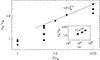 |
Fig. 12. Dependence of ϵK/ϵM on PrM. The solid line denotes |

Although 2D and 3D runs are in many ways rather different from each other, we now determine the same diagnostics as in the 3D case (see Table 3 and Fig. 13 for a plot of CM versus Lu). We see that the CM dependence on Lu is qualitatively similar for 2D and 3D turbulence. Moreover, it becomes shallower for larger values of Lu. There is now evidence that CM levels off and becomes independent of Lu. It is possible to fit our data to a function of the form
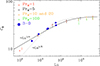 |
Fig. 13. Dependence of CM on Lu for the 2D runs. Shallow scaling ∝Lu0.1 is found for 104 < Lu < 105, which is also compatible with a leveling off at Luc = 2.5 × 10⁴, as described by Eq. (24) with n = 1/4. The black (red) data points are for PrM = 5 (PrM = 1). The blue data points denote the 3D results from Sect. 4. The orange symbols are for the runs with PrM = 10 and 20, listed in Table 3. The thin dotted line gives Eq. (24) with n = 1/4 for comparison. |
where Luc = 2.5 × 10⁴ is a critical Lundquist number characterizing the point where the dependence levels off, n = 1/4, and  . The value of Luc is larger than that found by Loureiro et al. (2012), where the asymptotes for small and large Lundquist numbers cross at a value closer to 5000. However, this difference could simply be related to different definitions of the relevant length scales. We note that our definition of ξM does not include a 2π factor. A comparison with the Sweet–Parker value of n = 1/2 results in reasonable agreement for small values of Lu, but there are rather noticeable departures from the data for intermediate values.
Our 2D and 3D results for CM are seen to be in good agreement with each other, which is similar to the observation made by Bhat et al. (2021). Obviously, larger simulations should still be performed to see whether the agreement between 2D and 3D continues to larger Lundquist numbers.
It should also be noted that some of our data with their nominal error bars do not lie on the fit given by Eq. (24) with n = 1/4. Especially for PrM = 100 and smaller values of Lu, we see that CM lies systematically below the fit. It should be noted, however, that we would expect an increase with PrM as (1 + PrM)1/2, which is the opposite trend, if the reconnection phenomenology were applicable (see Eq. (16) in Hosking & Schekochihin 2023).
To check whether our simulations are sufficiently well resolved, we show in Fig. 14 a visualization of Jz(x, y) for Run 2m6 with PrM = 10 and 163842 mesh points at t = 464 for a small part of the domain with sizes 2.8ξM(t)×0.74ξM(t) where a large current sheet breaks up into smaller plasmoids. A comparison between Runs 2m5 and 2m6 with 81922 and 163842 mesh points is shown in Appendix B. Our main conclusions are that higher resolution suppresses the tendency to produce ringing (i.e., the formation of oscillations on the grid scale), but that the results for CM are not very sensitive to the numerical resolutions, as can be seen by comparing Runs 2m5 and 2m6 in Table 3.
 |
Fig. 14. Visualization of Jz(x, y) of Run 2m6 with PrM = 10, Lu = 1.8 × 10⁵, Luν ≈ 5 × 10⁴, and 163842 mesh points at t = 464 for a small part of the domain with sizes 2.8ξM(t)×0.74ξM(t). The lengths of 100 δc, 2Lc, and ξM are indicated by horizontal white solid, dashed, and dotted lines, respectively. The thickness of the current sheet corresponds to about 3Δx ≈ 21 δc. In its proximity, there are also indications of ringing, indicated by the black circle. |
Next, we compare the typical length and thickness of current sheets in Run 2m6 with the values defined by Uzdensky et al. (2010) for critical current sheets, Lc = Luc η/vA and  , respectively. These lengths are indicated in Fig. 14. Here we used Luc = 2.5 × 10⁴ as the critical Lundquist number, which was found to be representative of all of our cases. We see that the current sheets in Fig. 14 have a length that is comparable to ξM ≈ 7 Lc, because Lu ≈ 7 Luc. The thickness of the current sheets is about 20 δc. They are marginally resolved with about 3Δx, where Δx = 2π/16384 ≈ 3.8 × 10⁻⁴ is the mesh spacing. Thus, the aspect ratio of thickness to length of the current sheets is about
  . This is about three times the nominal value estimated by Uzdensky et al. (2010) for critical current sheets.
By comparison, Hosking & Schekochihin (2023) estimated for the aspect ratio  . For Run 2m6 with Luν ≈ 5 × 10⁴, this yields 0.003, which is about six times smaller than our value of 0.02. While these discrepancies could perhaps be explained by the absence of nondimensional prefactors in the definitions of δc, we must also consider the possibility that this is simply a consequence of a lack of resolution.
Runs 2m2 and 2m6 have in common that they have the same resistivity and nearly the same value of Lu of about 1.8 × 10⁵, but Run 2m2 has a tenfold larger viscosity than Run 2m6, so PrM is increased from 10 to 100. We see that CM has deceased by only about 15%, which is much less than what is expected if CM was proportional to  .
.
In Fig. 15 we show for Runs 2m2 and 2m6 magnetic field profiles, −Bx(y) and By(y), and velocity profiles, −ux(y) and uy(y), through a particular current sheet. We see that in Run 2m2 with PrM = 100, the profiles are much smoother, even though the value of Lu = 1.8 × 10⁵ is the same in both cases. Thus, the viscosity has a significant effect in smoothing the magnetic field. Even so, the effect on the value of CM is small.
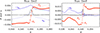 |
Fig. 15. Magnetic field profiles [−Bx(y) and By(y) in red] and velocity profiles [−ux(y) and uy(y) in blue] through the current sheet (in black) for Run 2m2 (through x = 0.372) and Run 2m6 (through x = 0.270). |
7. Endpoints in the primordial evolutionary diagram
The evolution of primordial magnetic fields is usually displayed in an evolutionary diagram showing the comoving values of Brms versus ξM or, similarly, vA versus ξM. This dependence corresponds to a power law of the form vA = vA0(ξM/ξM0)κ. Since ξM(t)∼tq, we have  , so κ = p/2q = 5/4 for the Hosking scaling with p = 10/9 and q = 4/9.
Following Banerjee & Jedamzik (2004), the time t in Eq. (10) would be replaced by the age of the Universe at the time of recombination, trec. As emphasized by Hosking & Schekochihin (2023), this gives an implicit equation for the magnetic field at recombination with the solution B(trec)≈10−8.5 G (ξM/1 Mpc) = 10−14.5 G (ξM/1 pc) if CM = 1. However, B(trec) would be much larger and ξM much smaller when CM ≫ 1 is taken into account.
Under the hypothesis of fast reconnection owing to plasmoid instability (Bhattacharjee et al. 2009; Uzdensky et al. 2010), Hosking & Schekochihin (2023) estimated CM as the square root of an effective cutoff value of about 104 for the Lundquist number and an additional factor of  . Here, they estimated PrM ≈ 107, so CM = 105.5 and B(trec)≈10−3 G (ξM/1 Mpc) = 10−9 G (ξM/1 pc).
Our new results challenge the reliability of the anticipated dependence of CM on PrM. With the current results at hand, Fig. 13 suggests that CM never exceeds the value  , even for PrM as large as 100. Particularly important is the fact that this result is independent of PrM. Given that Hosking & Schekochihin (2023) used PrM ≈ 107, which yielded an extra 103.5 factor, and therefore CM = 105.5 in their estimate, our new findings imply that the resistivity effect is actually independent of PrM. Although this has so far only been verified for values of PrM ≤ 5, we suggest that a more accurate formula for the endpoints of the evolution with CM = 47 ≈ 101.7 would be B(trec)≈10−6.8 G (ξM/1 Mpc) = 10−12.8 G (ξM/1 pc). These values are still above the lower limits inferred from suppressed GeV photon emission from the halos of blazars (Neronov & Vovk 2010).
8. Conclusions
The present results have shown that, up to the largest Lundquist numbers accessible to our present direct numerical simulations with 20483 mesh points, the decay times depend on the resistivity. Only for our 2D simulations do we see evidence for a cutoff. The dependence of hydromagnetic turbulence properties on the value of the resistivity is unusual for fully developed turbulence. We wonder whether our results reflect just a peculiar property of decaying turbulence or whether there could also exist aspects of statistically stationary turbulence that depend on the microphysical resistivity. Possible examples of resistively controlled time dependences could include the time that is needed to develop the final saturated magnetic energy spectrum in kinetically forced turbulence, where the magnetic field emerges due to a dynamo action (Haugen et al. 2003; Schekochihin et al. 2004). A resistively slow adjustment phase is reminiscent of what occurs for helical magnetic fields (Brandenburg 2001), where it has also been possible to measure a weak resistivity dependence of the turbulent magnetic diffusivity (Brandenburg et al. 2008).
In the present 3D case, the magnetic helicity vanishes on the average. However, in the spirit of the Hosking phenomenology of a decay controlled by the conservation of the Hosking integral, it is very possible, even in decaying turbulence, that the conservation of magnetic helicity in patches of one sign of magnetic helicity plays an important role in causing the resistively controlled decay speed. Whether or not this is equivalent to talking about reconnection remains an open question. As discussed in Sect. 2, the idea of reconnection in terms of current sheets and plasmoids may not be fully applicable in the context of turbulence, where magnetic structures are more volume filling than in standard reconnection experiments (see Fig. 2). Additional support for a possible mismatch between classical reconnection theory and turbulent decay times comes from our numerical finding that the dependence of CM on Lu seems to be independent of the value of PrM (see Fig. 13). More extensive numerical studies with resolutions of 81923 meshpoints, which was the resolution needed to see a leveling off in 2D, might suffice to verify our 2D findings in the 3D case.
Our present work motivates possible avenues for future research. One choice is to do the same for turbulence with a −αu friction term in the momentum equation. Such calculations were already performed by Banerjee & Jedamzik (2004) and the friction term is also incorporated in the phenomenology of Hosking & Schekochihin (2023). This is to model the drag from photons when their mean-free path begins to exceed the scale ξM. This is the case after the time of recombination, when it contributes to dissipating kinetic energy and leads to a decoupling of the magnetic field. The field then becomes static and remains frozen into the plasma. According to the work of Hosking & Schekochihin (2023), this results in a certain reduction of CM compared to the resistively limited value. Verifying this with simulations would be particularly important.
Another critical aspect to verify is the absence of a dependence of CM on PrM over a broader range of parameter combinations. Given that there are always limitations on the resolution, it may be useful to explore simulations in rectangular domains to cover a larger range of scales. Other possibilities include simulations with time-dependent values of η and ν to obtain a larger separation between ξM and the dissipation scale near the end of the simulation. However, there is the danger that artifacts are introduced that need to be carefully examined. Ill-understood artifacts can also be introduced by using hyperviscosity and hyperresistivity, which are used in some simulations. For the time being, however, the possibility of a PrM dependence of CM cannot be confirmed from our simulations. Whether or not this automatically rules out reconnection as the reason for a resistively limited value of CM, instead of the idea of magnetic helicity conservation in smaller patches, remains uncertain.
As the value of PrM is increased, we also see a systematic increase in the kinetic-to-magnetic dissipation ratio, ϵK/ϵM. Such a dependence has previously been seen for kinetically dominated forced turbulence, but it is shown here, perhaps for the first time, for magnetically dominated decaying turbulence. While such results may be of interest to the problem of coronal heating, it should be remembered that the present simulations have large plasma betas (i.e., the gas pressure dominates over the magnetic pressure). It would therefore be of interest to check whether the obtained PrM-dependence also persists for smaller plasma beta. The restriction to two dimensions is another computational simplification that allowed significantly larger Lundquist numbers to be accessed, but it needs to be checked that the results for ϵK/ϵM are not very sensitive to this restriction. Comparing the 3D Runs M1 and M3 of Table 1 with the 2D Run 2M3 of Table 3, which have PrM = 5 and similar Lundquist numbers, we see that the 2D results may overestimate the ratio ϵK/ϵM by a factor of about two. Future work will need to show whether this can also be confirmed for other parameters.
Acknowledgments
We thank Pallavi Bhat (Bangalore) and David Hosking (Princeton) for detailed comments and suggestions, especially regarding reconnection in the 2D case. We are also acknowledge inspiring discussions with the participants of the program on “Turbulence in Astrophysical Environments” at the Kavli Institute for Theoretical Physics in Santa Barbara. We are also grateful to Sébastien Galtier, Romain Meyrand, Annick Pouquet, and Alex Schekochihin for their interest in shedding light on the origin of the word anastrophy; see Appendix A. This research was supported in part by the Swedish Research Council (Vetenskapsrådet) under Grant No. 2019-04234, the National Science Foundation under Grant No. NSF PHY-1748958, a NASA ATP Award 80NSSC22K0825, and the Munich Institute for Astro-, Particle and BioPhysics (MIAPbP), which is funded by the Deutsche Forschungsgemeinschaft (DFG, German Research Foundation) under Germany’s Excellence Strategy – EXC-2094 – 390783311. We acknowledge the allocation of computing resources provided by the Swedish National Allocations Committee at the Center for Parallel Computers at the Royal Institute of Technology in Stockholm. F.V. acknowledges partial financial support from the Cariplo “BREAKTHRU” funds Rif: 2022–2088 CUP J33C22004310003. Software and data availability. The source code used for the simulations of this study, the PENCIL CODE (Pencil Code Collaboration 2021), is freely available on https://github.com/pencil-code/. The DOI of the code is https://doi.org/10.5281/zenodo.2315093. The simulation setups and corresponding data are freely available on https://doi.org/10.5531/sd.astro.9 (Brandenburg et al. 2024) and https://doi.org/10.5281/zenodo.10527437.
References
- Armua, A., Berera, A., & Calderón-Figueroa, J. 2023, Phys. Rev. E, 107, 055206 [CrossRef] [Google Scholar]
- Banerjee, R., & Jedamzik, K. 2004, Phys. Rev. D, 70, 123003 [NASA ADS] [CrossRef] [Google Scholar]
- Batchelor, G. K. 1953, The Theory of Homogeneous Turbulence (Cambridge University Press) [Google Scholar]
- Baym, G., Bödeker, D., & McLerran, L. 1996, Phys. Rev. D, 53, 662 [NASA ADS] [CrossRef] [Google Scholar]
- Bhat, P., Zhou, M., & Loureiro, N. F. 2021, MNRAS, 501, 3074 [CrossRef] [Google Scholar]
- Bhattacharjee, A., Huang, Y.-M., Yang, H., & Rogers, B. 2009, Phys. Plasmas, 16, 112102 [Google Scholar]
- Biskamp, D., & Müller, W.-C. 1999, Phys. Rev. Lett., 83, 2195 [NASA ADS] [CrossRef] [Google Scholar]
- Brandenburg, A. 2001, ApJ, 550, 824 [Google Scholar]
- Brandenburg, A. 2014, ApJ, 791, 12 [NASA ADS] [CrossRef] [Google Scholar]
- Brandenburg, A., & Kahniashvili, T. 2017, Phys. Rev. Lett., 118, 055102 [NASA ADS] [CrossRef] [Google Scholar]
- Brandenburg, A., & Oughton, S. 2018, Astron. Nachr., 339, 641 [Google Scholar]
- Brandenburg, A., & Rempel, M. 2019, ApJ, 879, 57 [NASA ADS] [CrossRef] [Google Scholar]
- Brandenburg, A., Enqvist, K., & Olesen, P. 1996, Phys. Rev. D, 54, 1291 [NASA ADS] [CrossRef] [Google Scholar]
- Brandenburg, A., Rädler, K.-H., Rheinhardt, M., & Subramanian, K. 2008, ApJ, 687, L49 [Google Scholar]
- Brandenburg, A., Kahniashvili, T., & Tevzadze, A. G. 2015, Phys. Rev. Lett., 114, 075001 [NASA ADS] [CrossRef] [Google Scholar]
- Brandenburg, A., Kahniashvili, T., Mandal, S., et al. 2017, Phys. Rev. D, 96, 123528 [NASA ADS] [CrossRef] [Google Scholar]
- Brandenburg, A., Sharma, R., & Vachaspati, T. 2023, J. Plasma Phys., 89, 905890606 [CrossRef] [Google Scholar]
- Brandenburg, A., Neronov, A., & Vazza, F. 2024, Datasets of Resistively Controlled Primordial Magnetic Turbulence Decay, American Museum of Natural History, http://dx.doi.org/10.5531/sd.astro.9 [Google Scholar]
- Cheng, B., & Olinto, A. V. 1994, Phys. Rev. D, 50, 2421 [CrossRef] [Google Scholar]
- Christensson, M., Hindmarsh, M., & Brandenburg, A. 2001, Phys. Rev. E, 64, 056405 [NASA ADS] [CrossRef] [Google Scholar]
- Comisso, L., & Bhattacharjee, A. 2016, J. Plasma Phys., 82, 595820601 [CrossRef] [Google Scholar]
- Comisso, L., & Sironi, L. 2019, ApJ, 886, 122 [Google Scholar]
- Comisso, L., Grasso, D., & Waelbroeck, F. L. 2015, Phys. Plasmas, 22, 042109 [CrossRef] [Google Scholar]
- Craig, I. J. D., & McClymont, A. N. 1991, ApJ, 371, L41 [NASA ADS] [CrossRef] [Google Scholar]
- Craig, I. J. D., Litvinenko, Y. E., & Senanayake, T. 2005, A&A, 433, 1139 [NASA ADS] [CrossRef] [EDP Sciences] [Google Scholar]
- Durrer, R., & Caprini, C. 2003, JCAP, 2003, 010 [CrossRef] [Google Scholar]
- Dwivedi, S., Anandavijayan, C., & Bhat, P. 2024, arXiv e-prints [arXiv:2401.01965] [Google Scholar]
- Falkovich, G. 1994, Phys. Fluids, 6, 1411 [NASA ADS] [CrossRef] [Google Scholar]
- Fyfe, D., & Montgomery, D. 1976, J. Plasma Phys., 16, 181 [CrossRef] [Google Scholar]
- Galishnikova, A. K., Kunz, M. W., & Schekochihin, A. A. 2022, Phys. Rev. X, 12, 041027 [NASA ADS] [Google Scholar]
- Galsgaard, K., & Nordlund, Å. 1996, J. Geophys. Res., 101, 13445 [NASA ADS] [CrossRef] [Google Scholar]
- Galtier, S., & Meyrand, R. 2015, J. Plasma Phys., 81, 325810106 [CrossRef] [Google Scholar]
- Hatori, T. 1984, J. Phys. Soc. Jpn, 53, 2539 [CrossRef] [Google Scholar]
- Haugen, N. E. L., Brandenburg, A., & Dobler, W. 2003, ApJ, 597, L141 [Google Scholar]
- Hosking, D. N., & Schekochihin, A. A. 2021, Phys. Rev. X, 11, 041005 [NASA ADS] [Google Scholar]
- Hosking, D. N., & Schekochihin, A. A. 2023, Nat. Comm., 14, 7523 [NASA ADS] [CrossRef] [Google Scholar]
- Kahniashvili, T., Tevzadze, A. G., Brandenburg, A., & Neronov, A. 2013, Phys. Rev. D, 87, 083007 [CrossRef] [Google Scholar]
- Kowal, G., Lazarian, A., Vishniac, E. T., & Otmianowska-Mazur, K. 2009, ApJ, 700, 63 [Google Scholar]
- Lazarian, A., & Vishniac, E. T. 1999, ApJ, 517, 700 [Google Scholar]
- Lazarian, A., Eyink, G. L., Jafari, A., et al. 2020, Phys. Plasmas, 27, 012305 [NASA ADS] [CrossRef] [Google Scholar]
- Liu, Y.-H., Cassak, P., Li, X., et al. 2022, Comm. Phys., 5, 97 [NASA ADS] [CrossRef] [Google Scholar]
- Loureiro, N. F., Samtaney, R., Schekochihin, A. A., & Uzdensky, D. A. 2012, Phys. Plasmas, 19, 042303 [NASA ADS] [CrossRef] [Google Scholar]
- Neronov, A., & Vovk, I. 2010, Science, 328, 73 [NASA ADS] [CrossRef] [Google Scholar]
- Parker, E. N. 1957, J. Geophys. Res., 62, 509 [Google Scholar]
- Pencil Code Collaboration (Brandenburg, A., et al.) 2021, J. Open Source Softw., 6, 2807 [Google Scholar]
- Pouquet, A. 1978, J. Fluid Mech., 88, 1 [NASA ADS] [CrossRef] [Google Scholar]
- Pouquet, A. 1993, in Les Houches Summer School on Astrophysical Fluid Dynamics, Session XLVII, eds. J. P. Zahn and J. Zinn-Justin (Amsterdam: Elsevier), 139 [Google Scholar]
- Rappazzo, A. F., Velli, M., Einaudi, G., & Dahlburg, R. B. 2007, ApJ, 657, L47 [Google Scholar]
- Rappazzo, A. F., Dahlburg, R. B., Einaudi, G., & Velli, M. 2018, MNRAS, 478, 2257 [NASA ADS] [CrossRef] [Google Scholar]
- Saffman, P. G. 1967, J. Fluid Mech., 27, 581 [Google Scholar]
- Schekochihin, A. A. 2022, J. Plasma Phys., 88, 155880501 [NASA ADS] [CrossRef] [Google Scholar]
- Schekochihin, A. A., Cowley, S. C., Taylor, S. F., Maron, J. L., & McWilliams, J. C. 2004, ApJ, 612, 276 [NASA ADS] [CrossRef] [Google Scholar]
- Sweet, P. A. 1958, in Electromagnetic Phenomena in Cosmical Physics, ed. B. Lehnert, IAU Symp., 6, 123 [NASA ADS] [Google Scholar]
- Tronko, N., Nazarenko, S. V., & Galtier, S. 2013, Phys. Rev. E, 87, 033103 [CrossRef] [Google Scholar]
- Uzdensky, D. A., & Loureiro, N. F. 2016, Phys. Rev. Lett., 116, 105003 [NASA ADS] [CrossRef] [Google Scholar]
- Uzdensky, D. A., Loureiro, N. F., & Schekochihin, A. A. 2010, Phys. Rev. Lett., 105, 235002 [Google Scholar]
- Vachaspati, T. 1991, Phys. Lett. B, 265, 258 [NASA ADS] [CrossRef] [Google Scholar]
- Vakoulenko, M. O. 1993, J. Plasma Phys., 50, 45 [CrossRef] [Google Scholar]
- Zhou, M., Wu, D. H., Loureiro, N. F., & Uzdensky, D. A. 2021, J. Plasma Phys., 87, 905870620 [NASA ADS] [CrossRef] [Google Scholar]
- Zhou, H., Sharma, R., & Brandenburg, A. 2022, J. Plasma Phys., 88, 905880602 [CrossRef] [Google Scholar]
- Zrake, J. 2014, ApJ, 794, L26 [NASA ADS] [CrossRef] [Google Scholar]
Appendix A: Historical note on anastrophy
In recent years, the term anastrophy for the mean squared magnetic vector potential  has become increasingly popular (Tronko et al. 2013; Galtier & Meyrand 2015; Zhou et al. 2021; Hosking & Schekochihin 2021; Schekochihin 2022). In the 1970s, it was referred to as mean square vector potential (Fyfe & Montgomery 1976) or as the variance of the magnetic potential (Pouquet 1978). The term anastrophy was first used in the 1987 Les Houches lecture notes by Pouquet (1993), and it was also used by Vakoulenko (1993), but neither of them provided an explanation of its origin.
Annick Pouquet (2024, private communication) informed us now that the word may have been invented by Uriel Frisch and Nicolas Papanicolaou during a meeting on a Winter Sunday in the late 1970s at Saint-Jean-Cap-Ferrat, while she and Jacques Léorat were also present.
The word has Greek roots, where ‘strophe’ refers to curl or turning, and ‘ana’ therefore hints at the inverted curl of B. This is somewhat reminiscent of the word palinstrophy, which is the mean squared double curl of the velocity, where ‘palin’ means again. This term was also invented by Frisch and Papanicolaou. The palinstrophy is proportional to the rate of change of enstrophy, i.e., the mean squared vorticity.
Appendix B: Resolving the plasmoid instability
The expected thickness of critical layers (i.e., the minimum thickness of current sheets when they become unstable to the plasmoid instability) is expected to be on the order of δc (see Sect. 6). To compare this with our 2D simulations, we show in Fig. 10 visualizations of Jz(x, y) in parts of the full domain with sizes 5ξM × 10ξM at times t = 1, 10, 100, and 464. We note that ξM(t) increases with time, so the x and y ranges increase with time too. We see that each panel contains about one pair of current tubes. Furthermore, the other length scales, Lc and δc, increase with time by the same factor, as expected for a self-similar evolution.
At late times, for t = 100 and 464, the current sheets are seen to break up into plasmoids. They are obviously better resolved in Run 2m6 with 163842 mesh points than in Run 2m5 with only 81922 mesh points. At lower resolution, there is a higher tendency for ringing (i.e., the formation of oscillations on the grid scale), which indicates that the resolution limit has been reached. Nevertheless, Table 3 and Fig. 13 show that, within the error bars, the values of CM are similar for the two resolutions.
It is possible that the critical current sheets are not well resolved during a significant fraction of the duration of the simulation. Theoretically, we expect the thinnest sheets to set the reconnection rate, but this is also the place where the value of PrM matters because viscosity is unimportant for the larger scales in the plasmoid hierarchy. Therefore, if we do not resolve that sheet, it seems reasonable that we would also not see a dependence on PrM. To check this, we now consider a version of Run 2m2, where the viscosity is ten times larger, which increases PrM from 10 to 100; see Run 2m6. The result is shown in Fig. B.1. We see that a lower value of Lu for PrM = 100 changes the results in an expected fashion, thus rejecting the possibility that the weak dependence of CM on PrM was an artifact of having chosen unreliably large values of Lu; compare Runs 2m1 and 2m2 in Fig. B.2.
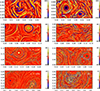 |
Fig. B.1. Comparisons of visualizations of Jz(x, y) for Runs 2m5 and 2m6 with PrM = 10 and 81922 (left) and 163842 (right) mesh points at times t = 1, 10, 100, and 464. In each panel the lengths of the dotted, dashed, and solid lines denote the values of ξM, 5 Lc, and 500 δc. The bottom right panel shows the same current sheet that was presented in Fig. 14 as a blow-up. The thick white line in that panel at (x, y) = (0.27, 0.25) marks the location of the cross section shown in Fig. 15. |
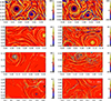 |
Fig. B.2. Similar to Fig. B.1, but for Run 2m1 with Lu = 75, 000 (left) and Run 2m2 with Lu = 182, 000 (right) using PrM = 100 and 163842 mesh points in both cases. The thick white line in the bottom right panel at (x, y) = (0.37, 0.25) marks the location of the cross section shown in Fig. 15. |
In the bottom right panel of Fig. B.1, we see the same current sheet that was already presented in Sect. 6 as Fig. 14. However, we also see in Fig. B.1 that there are many other current sheets that are not yet in the process of breaking up.
All Tables
All Figures
|
Fig. 1. Visualization of Bz on the periphery of the computational domain for Run M1, where PrM = 5. |
| In the text | |
|
Fig. 2. Visualization of Jz at z = π along with a zoom-in on the lower left corner for Run M0, where PrM = 10, at t = 644. The value of ξM at that time is indicated by the length of the short white lines. |
| In the text | |
|
Fig. 3. Magnetic and kinetic energy spectra for Run M1 at different times. For large values of k there is a k−2 inertial range. The ∝k4 and ∝k2 slopes are indicated for reference. As elsewhere, time is in units of [t]=(csk1)−1. |
| In the text | |
|
Fig. 4. Approach of CM(t), Lu(t), and |
| In the text | |
|
Fig. 5. Dependence of CM on Lu and Luν. An approximate scaling ∝Lu1/4 is found for Lu < 6000 and a piecewise power-law scaling |
| In the text | |
|
Fig. 6. Dependence of ℰM(t) and ξM(t) for three values of PrM. |
| In the text | |
|
Fig. 7. Evolution of τℰ(t) and τξ(t) for three values of PrM with fixed and moderate viscosity. These times tend to be approximately constant at late times with values approximately consistent with those in Table 1. |
| In the text | |
|
Fig. 8. Dependence of τξ and τℰ on Lu. The two show a similar dependence on Lu, approximately ∝Lu1/4, but there is possible evidence for a leveling off for larger values of Lu. |
| In the text | |
|
Fig. 9. Dependence of CK on Re. The line Re0.1 is shown for comparison, but the data are also nearly compatible with being independent of Re. |
| In the text | |
|
Fig. 10. Similar to Fig. 3, but for Run 2M1. The magnetic peaks lie underneath a kβ envelope with β = 1, as expected in the case of anastrophy conservation. |
| In the text | |
|
Fig. 11. Magnetic energy spectra (left) and kinetic energy spectra (right) for Run 2m2 with Lu = 1.8 × 10⁵ and PrM = 100, at times t = 5, 20, 100, and 400, collapsed on top of each other by plotting both vs kξM(t) and scaling them with ξM. This makes their heights agree, as expected. |
| In the text | |
|
Fig. 12. Dependence of ϵK/ϵM on PrM. The solid line denotes |
| In the text | |
|
Fig. 13. Dependence of CM on Lu for the 2D runs. Shallow scaling ∝Lu0.1 is found for 104 < Lu < 105, which is also compatible with a leveling off at Luc = 2.5 × 10⁴, as described by Eq. (24) with n = 1/4. The black (red) data points are for PrM = 5 (PrM = 1). The blue data points denote the 3D results from Sect. 4. The orange symbols are for the runs with PrM = 10 and 20, listed in Table 3. The thin dotted line gives Eq. (24) with n = 1/4 for comparison. |
| In the text | |
|
Fig. 14. Visualization of Jz(x, y) of Run 2m6 with PrM = 10, Lu = 1.8 × 10⁵, Luν ≈ 5 × 10⁴, and 163842 mesh points at t = 464 for a small part of the domain with sizes 2.8ξM(t)×0.74ξM(t). The lengths of 100 δc, 2Lc, and ξM are indicated by horizontal white solid, dashed, and dotted lines, respectively. The thickness of the current sheet corresponds to about 3Δx ≈ 21 δc. In its proximity, there are also indications of ringing, indicated by the black circle. |
| In the text | |
|
Fig. 15. Magnetic field profiles [−Bx(y) and By(y) in red] and velocity profiles [−ux(y) and uy(y) in blue] through the current sheet (in black) for Run 2m2 (through x = 0.372) and Run 2m6 (through x = 0.270). |
| In the text | |
|
Fig. B.1. Comparisons of visualizations of Jz(x, y) for Runs 2m5 and 2m6 with PrM = 10 and 81922 (left) and 163842 (right) mesh points at times t = 1, 10, 100, and 464. In each panel the lengths of the dotted, dashed, and solid lines denote the values of ξM, 5 Lc, and 500 δc. The bottom right panel shows the same current sheet that was presented in Fig. 14 as a blow-up. The thick white line in that panel at (x, y) = (0.27, 0.25) marks the location of the cross section shown in Fig. 15. |
| In the text | |
|
Fig. B.2. Similar to Fig. B.1, but for Run 2m1 with Lu = 75, 000 (left) and Run 2m2 with Lu = 182, 000 (right) using PrM = 100 and 163842 mesh points in both cases. The thick white line in the bottom right panel at (x, y) = (0.37, 0.25) marks the location of the cross section shown in Fig. 15. |
| In the text | |
Current usage metrics show cumulative count of Article Views (full-text article views including HTML views, PDF and ePub downloads, according to the available data) and Abstracts Views on Vision4Press platform.
Data correspond to usage on the plateform after 2015. The current usage metrics is available 48-96 hours after online publication and is updated daily on week days.
Initial download of the metrics may take a while.