| Issue |
A&A
Volume 686, June 2024
|
|
|---|---|---|
| Article Number | A26 | |
| Number of page(s) | 14 | |
| Section | Astrophysical processes | |
| DOI | https://doi.org/10.1051/0004-6361/202348815 | |
| Published online | 27 May 2024 | |
Ponderomotive forces in magnetized nonthermal space plasmas due to cyclotron waves
1
Departmento de Física, Facultad de Ciencias, Universidad de Chile, Santiago, Chile
e-mail: This email address is being protected from spambots. You need JavaScript enabled to view it.
; This email address is being protected from spambots. You need JavaScript enabled to view it.
2
Facultad de Ingeniería y Ciencias, Universidad Adolfo Ibáñez, Santiago, Chile
e-mail: This email address is being protected from spambots. You need JavaScript enabled to view it.
Received:
1
December
2023
Accepted:
4
March
2024
Abstract
Context. The ponderomotive force is involved in a variety of space plasma phenomena characterized by the family of Kappa distributions. Therefore, evaluating these nonthermal effects in the ponderomotive force is required.
Aims. The Karpman–Washimi ponderomotive interaction due to cyclotron waves is evaluated for different space conditions considering low-temperature magnetized plasmas described by an isotropic Kappa distribution and with a wave propagation parallel to the background magnetic field.
Methods. We performed a brief analysis of the influence of the Kappa distribution in the dispersion relation for a low-temperature plasma expansion at the lowest order in which the thermal effects can be appreciated without considering the damping characteristics of the wave. The different factors of the ponderomotive force were obtained and analyzed separately as a function of the wavenumber, the spectral index κ, and the plasma beta.
Results. We found a relevant influence of the nonthermal effects in all factors of the ponderomotive force for magnetized plasmas. The effect of the Kappa distribution has been evaluated for a wide variety of space environments, such as the solar wind and the different regions of our magnetosphere, where it has been found that these results can be relevant for the solar wind, the magnetosheath, the plasma sheet, and the polar cusps. We also analyzed the role of the nonthermal effect in the induced Karpman–Washimi ponderomotive magnetization in the context of spatial plasmas and the total radiated power associated with it.
Conclusions. We find that even for nearly cold magnetized plasmas and waves far from the resonances, the effect of the kappa parameter in the ponderomotive force cannot be neglected. This suggests a significant role of the Kappa distribution in ponderomotive phenomena of space physics.
Key words: acceleration of particles / plasmas / waves / solar-terrestrial relations
© The Authors 2024
 Open Access article, published by EDP Sciences, under the terms of the Creative Commons Attribution License (https://creativecommons.org/licenses/by/4.0), which permits unrestricted use, distribution, and reproduction in any medium, provided the original work is properly cited.
This article is published in open access under the Subscribe to Open model. This email address is being protected from spambots. You need JavaScript enabled to view it. to support open access publication.
1. Introduction
Space plasma environments are constantly affected by wave-wave and wave-particle interactions. Indeed, the solar wind plasma and its interplanetary magnetic field are externally forcing our planetary magnetosphere by the excitation of waves and the penetration of particles that propagate, for example, through the magnetic field lines of the polar cusps and the nightside magnetotail (Lakhina 1990; Chen 1992) or by instabilities in the solar wind and the geomagnetic field that leads to the propagation of ultra-low frequency (ULF) waves in our magnetosphere (Hughes 2013; Di Matteo et al. 2022). Usually, these processes are studied for low-amplitude perturbations to simplify the analysis of the dynamics by treatment of linearized systems. Nevertheless, this approach does not take account of a variety of phenomena that occur in space plasmas when considering finite amplitude waves. Thus, when nonlinear terms are considered, a diversity of effects in space plasmas emerge, such as three-wave decay interactions, modulation instabilities, self-wave interactions, wave trapping, and density cavities, among others (see Wong 1982; Eliasson & Shukla 2006; Kamide & Chian 2007).
In addition, when nonlinear effects are relevant, we need a useful tool that allows us to mathematically describe the space physics dynamics between waves and particles. To solve this and to take account of the nonlinear perturbative terms of the electromagnetic fields that emerge in the Lorentz force, the concept of ponderomotive force has been developed and widely used (Kentwell & Jones 1987). Ponderomotive forces are time-averaged nonlinear forces that emerge from the interaction of quasi-monochromatic waves or spatially inhomogeneous monochromatic waves with plasma. They are a useful tool that enables the study of the complex dynamics due to the interaction of waves with plasma in a slow timescale concerning the carrier high frequency of the wave, which can simplify our understanding of some physical phenomena (Lundin & Guglielmi 2007). Due to this characteristic, the ponderomotive force has had great relevance in the study of phenomena that involve the interaction between waves and plasma in different environments. It has been widely used in lasers, where it causes self-focusing effects (Karpman & Washimi 1977; Washimi 1989; Rezapour et al. 2018; Gupta et al. 2022), in addition to having applications in phenomena such as laser ignition of controlled nuclear fusion (Hora 2007, 2016; Hora et al. 2014), among others.
The ponderomotive force also has significant applications in space physics and is responsible for a diversity of phenomena (see Lundin & Guglielmi 2007; Lundin & Lidgren 2022). It has been used to study the redistribution of plasma in the terrestrial magnetosphere and the acceleration of ions in the polar wind (Allan 1992; Li & Temerin 1993; Guglielmi & Lundin 2001; Lundin & Guglielmi 2007; Nekrasov & Feygin 2012, 2014; Guglielmi & Feygin 2023). Some of these theoretical models are inspired by measurements of the satellites Freja and Viking in the ionosphere (Lundin & Hultqvist 1989; Lundin et al. 1990); however, measurements are lacking in the Earth’s magnetosphere that confirm, experimentally, the main points exposed in these works, which have nonetheless proposed some indirect measurement methods based on the dependence of the foreshock locations on the orientation of the field lines of the interplanetary magnetic field (see Guglielmi & Feygin 2018).
In addition to the magnetosphere, the ponderomotive forces have also been studied on the Sun, where they are relevant to understanding the difference in ion composition between the photosphere and the solar corona (Laming 2004, 2015). They have also been suggested to explain the magnetic holes (MHs) and magnetic decreases (MDs) of the interplanetary magnetic field observed in the solar wind due to the interaction of the plasma with phase-steepened Alfvén waves (Tsurutani et al. 2002; Dasgupta et al. 2003). They are involved in the nonlinear coupling of large amplitude electromagnetic pump waves with low-frequency collisional modes in the ionosphere (Drake 1974; Stenflo 1990). Also, they have been utilized to explain the magnetic-field-aligned electron density compressions by dispersive shear Alfvén waves (DSAWs) observed by FREJA and FAST spacecraft in the magnetosphere (Stasiewicz et al. 2000; Shukla et al. 2004). The ponderomotive force interaction with plasmas can also act as a generator of slowly varying magnetic fields (Washimi & Watanabe 1977), which has been widely studied because of its importance in the magnetic field generation in laser-matter interaction and dense plasmas in astrophysical compact objects (Na & Jung 2009; Shukla et al. 2010; Jamil et al. 2019).
Because the electromagnetic perturbation of plasma generates the ponderomotive force, its characteristics depend as much on the wave modulation as on the interaction with the medium described by the dielectric tensor and its dispersion relation. At the same time, these macroscopic variables ultimately depend on the velocity distribution that characterizes the plasma. It is well known that in most space environments, the plasma is described by the family of Kappa distributions instead of being characterized by the Maxwellian distribution because it does not reach the thermal equilibrium due to its low-collision rate (Viñas et al. 2005; Nieves-Chinchilla & Viñas 2008; Yoon 2014; Espinoza et al. 2018; Lazar & Fichtner 2021; Eyelade et al. 2021; Lazar et al. 2023). This family of distributions depends on the κ parameter and can be considered as a generalization of the Maxwellian distribution that is recovered when κ tends to infinity. They have been widely observed experimentally in near-Earth space environments, in addition to being proposed as an explanation of a great variety of phenomena such as the heating of the corona by velocity filtration and the acceleration of the fast solar wind (Pierrard & Lazar 2010). In many space environments, the kappa parameter can have a low value in the interval of 2 to 7 (Livadiotis 2015). Even in the inner magnetosphere around the plasmapause, the kappa parameter can have a value of κ ∼ 10 (Kirpichev et al. 2021). The theoretical support of the Kappa distribution is still a reason for discussion in the scientific community, and some models have been developed in an attempt to explain this observation. Among them, an attempt has been made to extend statistical mechanics with what is known as superstatistics (Davis et al. 2019; Gravanis et al. 2020; Yoon 2021). Therefore, due to its great importance in the description of collisionless plasmas in space environments, its effect has to be evaluated when studying certain phenomena in space physics. Moreover, the nonthermal effects of the plasma described by the Kappa distribution can significantly affect the behavior of the ponderomotive force and thus the phenomena associated with it. Therefore, an investigation of the effect of the Kappa distribution in the ponderomotive force is required.
Indeed, a detailed analysis of the characteristics of ponderomotive forces in nonthermal unmagnetized plasmas has recently been developed (see Espinoza-Troni et al. 2023). An initial approach has been made in the study of the nonthermal effects in the ponderomotive force by including the contribution of the Kappa distribution on nonmagnetized plasmas considering the movement of electrons in a background of immobile ions. This approach demonstrated the importance of the kappa parameter in the interaction between plasmas and waves of inhomogeneous amplitude in time and the magnitude of the induced magnetic fields derived from this interaction. Also, those results show that for unmagnetized plasmas, the nonthermal effects are negligible for the spatial ponderomotive force when nonrelativistic thermal velocities are considered. Nevertheless, it is expected that by including other parameters that characterize the interaction of the plasma with the waves, a different behavior of the effect of the kappa parameter in the ponderomotive force could be obtained. Indeed, that work can be extended to study the case of magnetized plasmas. This case becomes more relevant in space physics, where the plasma is usually interacting with an external magnetic field. The purpose of this work is to give a detailed analysis of the effect of including the Kappa distribution in the ponderomotive force due to the interaction of magnetized plasmas with waves propagating parallel to the external magnetic field and to evaluate its implications in different space environments. We include the nonthermal effects in the ponderomotive force by expanding the dielectric tensor for Kappa distributions in low-temperature magnetized plasmas without considering the damping of the wave. Then, we compare the magnitude of the factors accompanying the different terms of the ponderomotive force for the Kappa and Maxwellian distribution for different values of the plasma beta and the ratio between the plasma frequency and gyrofrequency to model the different space conditions.
This article is organized as follows: Sect. 2, includes the nonthermal effects in the kinetic dielectric tensor, and we obtain asymptotic expressions for low temperatures. We also give a brief analysis of the influence of the kappa parameter in the solutions of the dispersion relations of waves propagating parallel to the external magnetic field. Then, in Sect. 3, we include the dielectric tensor in terms of the ponderomotive force, and we deduce its expressions. Later, we give a general analysis of the influence of the nonthermal effects for each term of the ponderomotive force and wave mode, and we compare our results with the thermal (Maxwellian) case. Also, we use this analysis to study the nonlinear perturbation of the magnetic field by the ponderomotive force produced by electromagnetic waves propagating parallel to the external magnetic field. In Sect. 4, we evaluate our results for different space environments for their typical plasma parameters. Finally, in Sect. 5, we summarize the main conclusions of this work.
2. Dispersion relation for thermal and nonthermal plasmas with low temperature
We consider a Kappa distribution for isotropic three-dimensional plasmas (Hellberg & Mace 2002; Yoon et al. 2006; Hau et al. 2009; Yoon 2012; Viñas et al. 2015; Lazar et al. 2016; Moya et al. 2020, among others)
 (1)
(1)
Here, ℱκs is the Kappa distribution for the species s, where ns is their number density,  is their thermal velocity, ms is their mass, and Ts is their temperature. Also, kB is the Boltzmann constant, and Γ is the gamma function.
In this section, we give a brief review of the dispersion relation for high-frequency waves propagating through low-temperature plasmas described by a Kappa distribution Eq. (1) and with a background magnetic field parallel to the wave propagation. As a first case, we consider only the dynamics of electrons with a static background of ions to achieve quasi-neutrality. Thus, we neglect the contribution of the ions in the dispersion relation. In other words, we consider frequencies much larger than the ion plasma frequency. Due to the larger mass of the ions in comparison to the electrons, this consideration is valid for many contexts. Nevertheless, in some cases in which the ponderomotive force is involved, such as in ULF waves, the contribution of the ions cannot be neglected (Guglielmi et al. 1999; Nekrasov & Feygin 2012; Guglielmi & Feygin 2018, 2023). For this last case, when the wave frequency is comparable to the ion plasma frequency, we obtain the ion cyclotron wave mode of propagation. Therefore, we analyzed the effect of the Kappa distribution for electron modes and ion cyclotron waves for a parallel propagation with the background magnetic field (Chen 1984), which will be useful as a first approximation in the study of the nonthermal effect in the ponderomotive force of magnetized plasmas. In addition, to delimit our investigation in this work, we focused our analysis on the right-handed mode of propagation for the electron waves and the left-handed mode of propagation for the ion cyclotron waves. A detailed deduction of the dielectric tensor and the dispersion relation for nonrelativistic magnetized plasma modeled by isotropic Kappa distributions can be found in Mace (1996). The dispersion relation for Kappa distributed plasmas has also been investigated in a variety of different contexts (Hellberg et al. 2009; Pierrard & Lazar 2010; Kourakis et al. 2012; Lazar et al. 2018). The dielectric tensor for magnetized plasmas can be deduced using kinetic theory by linearly perturbing the Vlasov equation. In this way, the same result as Hellberg & Mace (2002) is obtained, namely:
 (2)
(2)
where the upper sign is associated with the right-handed waves and the lower sign is for the left-handed waves. Here, ω is the frequency, k is the wave number, c is the velocity of light, ZκM is the modified generalized plasma dispersion function (see Appendix A), and ωps and Ωs are the plasma frequency and the gyrofrequency for the species s. We used ε± = ε11 ± iε12 as the eigenvalues of the dielectric tensor for the transversal modes of propagation, where εij are the components of the dielectric tensor with a magnetic field in the z direction. The dispersion relation is given by
 (3)
(3)
Since the longitudinal waves do not interact with the magnetic field, they remain the same as in the unmagnetized case analyzed for the ponderomotive force in Espinoza-Troni et al. (2023).
We considered low-temperature plasmas such that (ω ± Ωs)/kαs ≫ 1 for both ion and electron species. Under this approximation, we can make use of the asymptotic expansion of the generalized plasma dispersion function for large arguments and truncate the series at the lowest order in which the effect of the kappa parameter appears (see Appendix A) so that the temperature is included in the dielectric tensor. In this way, we expand in kαs/(ω ± |Ωs|) up to the second order in the dielectric tensor given by Eq. (2). As a first approach to the study of the nonthermal effects on the ponderomotive force for magnetized plasmas, we do not consider the imaginary terms (i.e., the damping characteristics of the wave in the expansion of the generalized plasma dispersion function), leaving them for future research. We can neglect the damping characteristics of the wave as long as we consider k−1(ω − |Ωs|) ≫ αs (Fitzpatrick 2015), which considering that due to our low-temperature approximation, we have low values of αs, this is then satisfied if the frequency is far from the resonances.
By considering the electron species and only one type of ion in Eq. (A.3), we obtained the approximated dielectric tensor components for electromagnetic waves in magnetized plasmas with parallel propagation (Chen 1984) and finite and low temperature as well as for right-handed (upper sign) and left-handed (lower sign) waves as follows
 (4)
(4)
Here, ε0±(ω) are the dielectric tensor eigenvalues for cold plasmas. The δ±(ω) factor is where the effect of the finite temperature is contained, and it is responsible for the spatial dispersion of the wave. These two quantities can be expressed as
 (5)
(5)
 (6)
(6)
From the previous equations, we can get the dispersion relation for electron cyclotron waves given by Eq. (10) by considering ω ≫ Ωi and ω ≫ ωpi. Also, we can obtain the ion cyclotron dispersion relation given by Eq. (12) by considering that me/mi ≪ 1 and ω < Ωi. In addition, we note that the expression Eq. (4) is necessary to deduce the temporal and magnetic moment ponderomotive factor before using the dispersion relation (see Appendix B).
By considering the dispersion relation given by Eq. (3) in Eq. (4), we can directly express the dielectric tensor eigenvalues as a function of the frequency, and we obtained ε±(ω, k(ω)) = ε0±(ω)/[1 + κ/(κ − 3/2)δ±(ω)]. Also, due to our low-temperature plasma approximation far from resonances, we had to consider that (ω − Ωs)/kαs ≫ 1, then δ± ≪ 1 for both electron waves and ion cyclotron waves. Hence, for the plasmas that we consider, we can use the following as a good approximation for the dielectric tensor eigenvalues:
![Mathematical equation: $$ \begin{aligned} \varepsilon _\pm (\omega ,k(\omega )) \approx \varepsilon _{0\pm }(\omega )\left[1-\left(\frac{\kappa }{\kappa -3/2}\right)\delta _{\pm }(\omega )\right]\cdot \end{aligned} $$](/articles/aa/full_html/2024/06/aa48815-23/aa48815-23-eq8.gif) (7)
(7)
We also note that we recovered the Maxwellian case in the limit κ → ∞. Therefore, using Eq. (3) in the previous equation, our approximation for the dispersion relation is given by
![Mathematical equation: $$ \begin{aligned} \frac{k^2c^2}{\omega ^2} = \varepsilon _{0\pm }(\omega ) \left[1-\left(\frac{\kappa }{\kappa -3/2}\right)\delta _{\pm }(\omega )\right]\cdot \end{aligned} $$](/articles/aa/full_html/2024/06/aa48815-23/aa48815-23-eq9.gif) (8)
(8)
Next, we review the main characteristics of the modes of propagation that we use in this work, and we limit the range of frequencies for which our approach is valid.
2.1. Electron cyclotron waves
As stated above, we can neglect ions as long as the ion plasma frequency is very low compared to the wave frequency ωpi ≪ ω (Krall & Trivelpiece 1986). Using this approximation in Eqs. (5) and (6) and considering the right-handed wave mode of propagation, we can obtain
 (9)
(9)
where y = ω/|Ωe| and  is the electron plasma beta, with B0 as the norm of the background magnetic field. We normalized the wavenumber as x = kc/ωpe. Then, using Eq. (9) in Eq. (8), our approximation for the dispersion relation for electron cyclotron waves was given by
![Mathematical equation: $$ \begin{aligned} \frac{x^2}{{ y}^2}\left(\frac{\omega _{\rm pe}^2}{\Omega _{\rm e}^2}\right) = \left[1-\frac{(\omega _{\rm pe}^2/\Omega _{\rm e}^2)}{{ y}({ y}-1)}\right]\left[1-\left(\frac{\kappa }{\kappa -3/2}\right)\frac{\beta _{\rm e}}{2}\frac{{ y}}{({ y}-1)^3}\right]. \end{aligned} $$](/articles/aa/full_html/2024/06/aa48815-23/aa48815-23-eq12.gif) (10)
(10)
We note that when we set βe = 0, that is, when we do not consider the finite temperature effects, we recovered the usual dispersion relation for cold magnetized plasmas with parallel wave propagation (Bittencourt 2010).
We numerically solved the dispersion relation given by Eq. (10), and we obtained two solutions for the right-handed mode of propagation, as we expected due to the cold case. One can see in Fig. 1 the electron cyclotron solution of the scaled frequency ω/|Ωe| as a function of the scaled wavenumber kc/ωpe for different electron plasma beta regimes and kappa values. For the higher frequency branch solution, which is not shown in Fig. 1, we have that for overdense plasmas, the effect of the Kappa distribution is not significant for βe < 10, with a relative difference that is at most on the order of 10−4 (not shown). Thus, we do not consider this solution in this work.
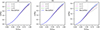 |
Fig. 1. Solution for the dispersion relation for right-handed electron cyclotron waves for y = ω/|Ωe| as a function of x = kc/ωpe with ωpe/|Ωe| = 30 for different values of κ, with (a) βe = 0.05, (b) βe = 0.1, and (c) βe = 0.5. |
In this paragraph, we clarify the range of the parameter values that we are taking into consideration. We note that our condition for the asymptotic expansion of the modified generalized plasma dispersion function is equivalent to  . Therefore, due to the dispersion relation, the validity of our approximation depends on the values of the wavenumber, the plasma beta, ωpe/|Ωe|, and the mode of propagation. For the electron cyclotron solution, the dependence of
  in the ratio of frequencies is negligible. Also, we neglect fourth order terms of ζ−1 = β1/2x/(1 − y) in Eq. (2). Hence, for our approximation to be consistent, we considered ζ−4 < 0.01. In Table 1, we have for different values of the wavenumber, the maximum beta value that accomplishes this condition for the electron cyclotron waves. One can see that for this mode of propagation, our results will be valid for larger values of the plasma beta as long as we consider lower values of the frequency. Also, in this work, we focus mainly on analyzing overdense plasmas with ω/|Ωe|> 10, which are typical values in space environments, as we show in Sect. 4. For that case, we have |ε0|≫1 for electron cyclotron waves, so we could use as a good approximation that
  .
.
Maximum value of the electron plasma beta βmax that accomplishes the condition ζ−4 < 0.01 for different values of the scaled wavenumber x for electron cyclotron waves.
Figure 2a shows the relative difference of the scaled frequency for the Kappa case and Maxwellian case yκ/yMB − 1 for the electron cyclotron waves, where the supra index κ indicates the frequency dependence in the kappa parameter and the supra index MB denotes the Maxwellian case (when κ → ∞). We maintain this index notation when analyzing the ponderomotive terms for nonthermal plasmas (see below). In the figure, one can notice that the dispersion relation varies appreciably concerning the kappa parameter at the order of 10−2 for the electron cyclotron waves for ωpe/|Ωe| = 30 and βe ∼ 10−1, which are typical values that can be found in space plasmas. We can also deduce that the kappa parameter has a greater influence on the electron cyclotron waves (inherent in the presence of the magnetic field) than the higher frequency solution. Hence, the nonthermal effect behaves very differently in the presence of a magnetic field. Also, for parallel wave propagation with the background magnetic field, the nonthermal effect gets enhanced with the plasma beta, as can be seen in Fig. 1. This can be explained because when the thermal pressure is larger than the pressure of the magnetic field, the electrons have more freedom to yield to thermal effects and escape the magnetic field confinement.
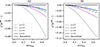 |
Fig. 2. Relative difference of the Kappa and Maxwellian scaled frequencies as a function of the scaled wavenumber for different values of the parameter Kappa (a) for electron cyclotron waves with βe = 0.1 and ωpe/|Ωe| = 30 and (b) for ion cyclotron waves with βi = 0.1 and cA/c = 10−3. |
2.2. Ion cyclotron waves
In this case, wave frequencies are comparable to the ion plasma frequency, and we thus have to consider the effect of the ion in the dispersion relation. Also, if we neglect terms on the order of me/mi < 10−3, we consider a quasi-neutral plasma and the left-handed mode of propagation in Eqs. (5) and (6). We then have that
 (11)
(11)
For this case, the scaled frequency is given by y = ω/Ωi, and the scaled wavenumber is given by x = kc/ωpi. Also,  is the Alfvén speed, with ρ = mene + mini ≈ mini as the plasma density, and
  is the ion plasma beta. Then, using Eq. (11) in Eq. (8), our approximation for the dispersion relation for ion cyclotron waves is given by
![Mathematical equation: $$ \begin{aligned} \frac{x^2}{{ y}^2}\left(\frac{c^2}{c_{\rm A}^2}\right) = \left[1 - \left(\frac{c}{c_{\rm A}}\right)^2 \frac{1}{({ y} - 1)}\right] \left[1-\frac{\beta _{\rm i}}{2}\left(\frac{\kappa }{\kappa -3/2}\right)\frac{{ y}}{({ y} - 1)^3}\right]\cdot \end{aligned} $$](/articles/aa/full_html/2024/06/aa48815-23/aa48815-23-eq19.gif) (12)
(12)
We have numerically solved this dispersion relation, which is shown in Fig. 3 for different ion plasma beta regimes and kappa parameters. We note that it has characteristics that are similar to the electron cyclotron dispersion relation shown in Fig. 1. The nonthermal effects are enhanced with the ion plasma beta, and the frequency decreases for lower values of the kappa parameter. As in the electron cyclotron waves, to accomplish our approximation, we work with the range of values for y given by Table 1. In space plasmas, since we have typical values of the Alfvén speed of cA/c ∼ 10−3 or ∼10−4 (Bourouaine et al. 2012; Kim et al. 2018), then |ε0|≫1, and we can use the following approximation of the dielectric tensor eigenvalue for ion cyclotron waves ε0 ≈ −(c/cA)2/(y − 1).
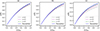 |
Fig. 3. Solution for the dispersion relation for left-handed ion cyclotron waves for y = ω/Ωi as a function of x = kc/ωpi, with c/cA = 102, for different values of κ with (a) βi = 0.05, (b) βi = 0.1, and (c) βi = 0.5. |
Finally, in Fig. 2b, we show the relative difference of the scaled frequency for the Kappa and Maxwellian case yκ/yMB − 1 for the ion cyclotron waves. We note that, as is the case with the electron cyclotron waves, the dispersion relation varies appreciably concerning the kappa parameter on the order of 10−2 for the ion cyclotron waves for cA/c = 10−3 and βi ∼ 10−1, which are typical values that can be found in space plasmas.
3. Ponderomotive force
The ponderomotive force is a nonlinear phenomenon induced by the interaction of a high-frequency field with the plasma in a slow timescale motion concerning the carrier frequency of the wave (Kentwell & Jones 1987). The purpose of this work is to study how the nonthermal effect described by the Kappa distribution impacts the nonlinear, slow timescale interaction of magnetized plasmas with electromagnetic fields. Currently, there is a great diversity of formalism regarding where the ponderomotive force is derived, and it has been extensively studied (see Kentwell & Jones 1987). In this discussion, we are going to use the Karpman–Washimi ponderomotive force and the previous results for the dispersion relations for low-temperature plasmas characterized by Kappa distributions. This formalism can be obtained either from a stress tensor or fluid formalism for a temporally dispersive and nonabsorbing medium (Washimi & Karpman 1976; Karpman & Shagalov 1982). Nevertheless, due to the fluid character of its derivation, this force does not work near resonances, where we know that for magnetized plasmas, the ponderomotive force produced by cyclotron waves can inject a large amount of energy in the plasma (see Lundin & Guglielmi 2007). In this regime, the fluid expression of the ponderomotive force diverges. Hence, the damping of the wave must be considered to counteract this effect. For this approach, a kinetic formalism must be used, which we leave for future research.
In the presence of a background magnetic field, the ponderomotive force of Karpman–Washimi fWK, due to the electromagnetic field ![Mathematical equation: $ \bar{\boldsymbol{E}}(\boldsymbol{r},t)\{=(1/2)[\boldsymbol{E}(\boldsymbol{r},t)e^{-i\omega t} + \boldsymbol{E}^*(\boldsymbol{r},t)e^{-i\omega t}]\} $](/articles/aa/full_html/2024/06/aa48815-23/aa48815-23-eq20.gif) , depends on a term f(s) associated with the spatial variation of the electric field magnitude, a term f(t) associated with the temporal variation of the electric field magnitude, a term f(m) associated with the magnetically induced moment current, and a term f(MMP) associated with the spatial variation of the background magnetic field:
, depends on a term f(s) associated with the spatial variation of the electric field magnitude, a term f(t) associated with the temporal variation of the electric field magnitude, a term f(m) associated with the magnetically induced moment current, and a term f(MMP) associated with the spatial variation of the background magnetic field:
 (13)
(13)
For this particular case, we can express the spatial factor of the ponderomotive force as follows (Washimi & Karpman 1976):
 (14)
(14)
If we also suppose that the magnitude of the electric field varies slowly in our time and space scales, it can be deduced that the temporal-variation part of the ponderomotive force becomes (Washimi & Karpman 1976)
 (15)
(15)
For this case, we can express the ponderomotive force associated with the currents induced by the ponderomotive magnetic moment as (Karpman & Shagalov 1982)
 (16)
(16)
where M = (1/16π)(∂ε±/∂B0)|E|2 is the nonlinear magnetic moment produced by the ponderomotive force,  is the background field, and
  is the gradient transverse to the magnetic field.
Finally, we have the term associated with the spatial variation of the background magnetic field, which is called magnetic moment pumping and can be considered as the force applied to a magnetic dipole due to an external magnetic field (Lundin & Guglielmi 2007):
 (17)
(17)
Next, we analyze the factors f(s){=(1/8π)(ε+−1)} and f(t){=(k/16πω2)[dω2(ε+ − 1)/dω]} that accompany the spatial and temporal variations of the magnitude of the electric field in the ponderomotive force and the magnetic moment, M, due to the propagation of electron cyclotron waves and ion cyclotron waves described by Kappa distributions.
3.1. Spatial ponderomotive force factor
For electron cyclotron waves, using our results for the dielectric eigenvalue ε+, we can deduce that the factor  that accompanies the spatial variation in the ponderomotive force for plasmas characterized by Kappa distributions is given by
 (18)
(18)
with y = ω/|Ωe| (see Appendix B for more details). Here, we note that if we neglect our finite temperature correction, that is, we put βe = 0 in Eq. (14), then we recover the spatial term of the ponderomotive force for electron cyclotron waves in cold plasmas (Lundin & Guglielmi 2007). Also, if we set |Ωe| = 0, considering that  , we recover the expression deduced for the spatial ponderomotive term in the unmagnetized case (Espinoza-Troni et al. 2023) (except here we consider that |ε0|≫1).
We note that the spatial term of the ponderomotive force is positive for the electron cyclotron waves (ω < |Ωe|). Therefore, the spatial term of the ponderomotive force will push the plasma along the gradient of the amplitude of the wave. Also, the ponderomotive force increases with the wavenumber (i.e., when approaching the resonance). Indeed, the solutions exhibit a resonance for ω = 0, where our results are not valid for electron cyclotron waves since we would have to consider the effect of the ions. Our Eq. (18) also shows a resonance in ω = |Ωe|. Nevertheless, this is not valid since we have considered as an approximation that δ ≪ 1. Hence, when we approach the resonances, we have to use the dispersion relation given by Eq. (2). The same observation can be extended to the other ponderomotive force terms. To study the resonances, we would also have to extend the formalism to include the damping of the wave. Moreover, the spatial term of the ponderomotive force has a minimum that is enhanced with the nonthermal effect and is shifted to lower frequencies.
Figure 4a shows the ratio of the Kappa and Maxwellian ponderomotive spatial factor  as a function of the scaled wavenumber ω/|Ωe| for the electron cyclotron waves. As it is seen, the magnitude of the ponderomotive force for the Kappa distributions is greater compared to the Maxwellian distribution case. It gets enhanced with the decrease of the kappa parameter. Besides, when the scaled wavenumber decreases, both magnitudes are equal, so the nonthermal effect is canceled. It is relevant to note that the relative difference of the Kappa and Maxwellian spatial factor is on the order of 10−2 for the electron cyclotron waves for βe = 0.1, and its dependence in ωpe/|Ωe| is very low (indeed, for our overdense plasmas approximation, |ε0|≫1 is independent of ωpe/|Ωe|). Unlike the unmagnetized case, where for nonrelativistic velocities of αe/c ∼ 10−2, we had no more than a relative difference on the order of 10−5 (Espinoza-Troni et al. 2023), so we can deduce that the effect of the kappa parameter in the ponderomotive force becomes more relevant when we include the effect of a background magnetic field in the plasma. Also, the nonthermal effect is larger for overdense plasmas. As we show below, these parameters of the plasma beta and the frequency ratio can be found in the solar wind, the near magnetotail, and the plasma sheet, so we can conclude that in these environments, the effect of the kappa parameter in the electron cyclotron ponderomotive force is significant, even for low-frequency waves. We also expect that the effect of the kappa parameter can be more notorious for larger values of the frequency and the plasma beta, for which we would have to relax our approximation.
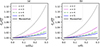 |
Fig. 4. Ratio of the Kappa and Maxwellian ponderomotive spatial factor |

For ion cyclotron waves, by using our result for the dielectric eigenvalue ε+, we can deduce that the factor  that accompanies the spatial variation in the ponderomotive force for plasmas characterized by Kappa distributions is given by
 (19)
(19)
with y = ω/Ωi. We note that as is the case for electron cyclotron waves, the spatial term of the ponderomotive force for ion cyclotron waves will push the plasma in favor of the gradient of the wave amplitude. For very low frequencies, ω ≪ Ωi, the nonthermal effects are canceled, and the spatial ponderomotive factor tends to be constant with an asymptotic value of (1/16π)(c/cA)2. Figure 4b shows the ratio of the Kappa and Maxwellian ponderomotive spatial factor  as a function of the scaled wavenumber ω/Ωi for the ion cyclotron waves. We have that the spatial term of the ponderomotive force for the ion cyclotron wave is enhanced with the kappa parameters at the same ratio as the electron cyclotron waves. This was expected because the δ term has the same form for both modes of propagation.
Due to the factor βe multiplying κ/(κ − 3/2), the nonthermal effect increases with the plasma beta in the low-plasma beta domain that we are analyzing for electron cyclotron waves and ion cyclotron waves. It could be expected because the larger the thermal effect on the magnetic field, the less confined the electrons in the path described by the magnetic field, as we discussed above when we analyzed the dispersion relation. Therefore, it is expected that the effect of the kappa parameter can be enhanced for larger values of the plasma beta, as can be found in the magnetic holes produced by the ponderomotive force of the steepened Alfvén waves in the solar wind, which can have values of β ∼ 1 (Dasgupta et al. 2003). For the dayside magnetosheath, we have values for the βi of ions between 1 and 13, with an average of βi ∼ 3.5. For these values, we would have to use the full expression of the generalized plasma dispersion function for ions, and we could use our approximation for electrons whose temperature is one order of magnitude lower. Nevertheless, when the magnetic shear between the magnetopause and the magnetosheath is low, this last region presents a transition layer to the magnetopause where the plasma beta can be lower than 1 for both species, reaching values of βi ∼ 0.4. Therefore, in this case, our approximation could be used while including ions (Phan et al. 1994). We also note that for β = 0.1, a scaled frequency of 0.3, and κ = 2, the spatial ponderomotive factor for both the electron cyclotron waves and the ion cyclotron waves is 12% larger than for Maxwellian plasmas. We therefore have a significant impact of the kappa parameter on the magnitude of the spatial term of the ponderomotive force, and its implications in space phenomena could be useful as a tool to make measurements of the kappa parameter and to get a better understanding of the velocity distribution in space environments.
3.2. Temporal ponderomotive force factor
Here we analyze the influence of the nonthermal effect in the factor  that accompanies the temporal variation of the wave amplitude in the ponderomotive force for electron cyclotron waves and ion cyclotron waves. We have for the electron cyclotron waves that
![Mathematical equation: $$ \begin{aligned} f_{\rm (t)}^\kappa = \frac{1}{16\pi c}\left(\frac{\omega _{\rm pe}}{|\Omega _{\rm e}|}\right)^3\frac{1}{{ y}^{3/2}(1-{ y})^{5/2}}\left[1+ \frac{\beta _{\rm e}}{4}\left(\frac{\kappa }{\kappa -3/2}\right)\frac{(3+4{ y}){ y}}{(1-{ y})^3} \right], \end{aligned} $$](/articles/aa/full_html/2024/06/aa48815-23/aa48815-23-eq37.gif) (20)
(20)
with y = ω/|Ωe|. From the previous equation, it follows that the temporal factor of the ponderomotive force is nonzero, even if we consider a zero temperature (i.e., for βe = 0), which is unlike what happens for unmagnetized plasmas (Espinoza-Troni et al. 2023) whose temporal ponderomotive term is canceled for cold plasmas.
We note that the temporal factor of the ponderomotive force is positive for the electron cyclotron waves. The direction of the temporal term of the ponderomotive force depends on the direction of the propagation of the wave and the temporal variation of the wave amplitude, as can be seen more clearly in Eq. (15). This force will push the plasma toward (away from) the wave propagation direction for the temporal increase (decrease) of the wave amplitude. As is the case of the spatial ponderomotive force term, the temporal force term increases with the wavenumber (i.e., when approaching the resonance).
Also, in this case, we have a minimum that decreases with the nonthermal effects and is shifted to lower frequencies. Figure 5a shows the ratio of the Kappa and Maxwellian ponderomotive temporal factor for right-handed electron cyclotron waves  as a function of the scaled frequency ω/|Ωe| for βe = 0.1. For overdense plasmas, one can notice in this figure that the ponderomotive temporal factor for electron cyclotron waves is larger for Kappa-distributed plasmas than for Maxwellian plasmas by an order of magnitude of ∼10−1. One can also notice that the ponderomotive temporal factor is proportional to (ωpe/|Ωe|)3.
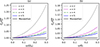 |
Fig. 5. Ratio of the Kappa and Maxwellian ponderomotive temporal factor |

Next, we analyze the ponderomotive temporal factor for ion cyclotron waves, which is given by
![Mathematical equation: $$ \begin{aligned} f_{\rm (t)}^\kappa = \frac{1}{16\pi c}\left(\frac{c}{c_{\rm A}}\right)^3 \frac{(2-{ y})}{(1-{ y})^{5/2}}\left[1+ \frac{\beta _{i}}{4}\left(\frac{\kappa }{\kappa -3/2}\right)\frac{(4+3{ y}){ y}}{(2-{ y})(1-{ y})^3} \right], \end{aligned} $$](/articles/aa/full_html/2024/06/aa48815-23/aa48815-23-eq40.gif) (21)
(21)
with y = ω/Ωi. We note that for very low frequencies, ω ≪ Ωi, the temporal ponderomotive factor tends toward a constant asymptotic value given by (1/8πc)(c/cA)3, where the finite temperature effects are canceled. Figure 5b shows the ratio of the Kappa and Maxwellian ponderomotive temporal factor for ion cyclotron waves  as a function of the scaled frequency ω/Ωi for βi = 0.1. We note that in this figure the ponderomotive temporal factor for ion cyclotron waves is larger for Kappa-distributed plasmas than for Maxwellian plasmas by an order of magnitude of ∼10−1. Also, for both the electron cyclotron and ion cyclotron waves, the nonthermal effect increases with the plasma beta, as we expected due to a less magnetic-confined plasma, as we discussed above.
Finally, we note that for β = 0.1, a scaled frequency of 0.3, and κ = 2, the temporal ponderomotive factor is 25% and 18% larger than for the Maxwellian plasmas of electron cyclotron waves and ion cyclotron waves, respectively. Therefore, the nonthermal effect can be significant when evaluating the temporal term of the ponderomotive force, even for low-temperature plasmas. On the other hand, this term can be relevant when we approach the resonances for what we would have to consider the damping of the wave, and therefore its amplitude would have a temporal variation. For that case, terms of the order of δ2 could not be neglected unless we consider low damping far from the resonances. As we show in Sect. 3.4, this temporal ponderomotive term also acts to perturb the slow timescale background magnetic field B0.
3.3. Magnetic moment of the ponderomotive force
In this section, we analyze the ponderomotive magnetic moment factor M = (1/16π)(∂ε/∂B)|E|2 produced by the wave propagation in Kappa-distributed plasmas, which is responsible for the induced current force and the MMP force of Eqs. (16) and (17). We obtained that the magnetic moment for a certain Kappa value Mκ for the electron cyclotron waves is given by
![Mathematical equation: $$ \begin{aligned} M^\kappa = -\frac{|E|^2}{16\pi B_0}\left(\frac{\omega _{\rm pe}}{|\Omega _{\rm e}|}\right)^2\frac{1}{{ y}(1-{ y})^2}\left[1 + \frac{3}{2}\beta _{\rm e}\left(\frac{\kappa }{\kappa -3/2}\right)\frac{{ y}}{(1-{ y})^3}\right], \end{aligned} $$](/articles/aa/full_html/2024/06/aa48815-23/aa48815-23-eq42.gif) (22)
(22)
where y = ω/|Ωe|. On the other hand, for ion cyclotron waves, we have that
![Mathematical equation: $$ \begin{aligned} M^\kappa = -\frac{|E|^2}{8\pi B_0}\left(\frac{c}{c_{\rm A}}\right)^2 \frac{(2-{ y})}{(1-{ y})^2}\left[1 + \frac{3}{2}\beta _{i}\left(\frac{\kappa }{\kappa -3/2}\right)\frac{{ y}}{(2-{ y})(1-{ y})^3}\right], \end{aligned} $$](/articles/aa/full_html/2024/06/aa48815-23/aa48815-23-eq43.gif) (23)
(23)
where y = ω/Ωi. We note that when ω ≪ Ωi, the ponderomotive magnetic moment tends toward an asymptotic value given by −(|E|2/8π)(c/cA)2, and the finite temperature effects are canceled. We also note that the ponderomotive magnetic moment is negative for both the electron cyclotron waves and the ion cyclotron waves. Therefore, the MMP term of the ponderomotive force will push the plasma against the gradient of the amplitude of the background magnetic field. For this reason, this force is responsible for the acceleration of ions in the polar cusps, where the ponderomotive force pushes the plasma out of the polar regions (Li & Temerin 1993; Guglielmi & Lundin 2001). It can also be seen that in both the cold- and low-temperature plasma cases, as we get closer to the resonance, the ponderomotive magnetic moment tends to be larger in the negative direction.
Figures 6a and b show the relative ratio of the ponderomotive magnetic moment M for Kappa and Maxwellian distributed plasmas as a function of the scaled frequency for electron cyclotron waves and ion cyclotron waves. We note that for both modes of propagation in the range of frequencies under consideration, the ponderomotive magnetic magnitude is larger for the Kappa case than the Maxwellian case. Also, we observed that even for low values of the plasma beta, the nonthermal effect is very significant for both the electron cyclotron waves and the ion cyclotron waves. Indeed for β = 0.1, we have that the ponderomotive magnetic moment for the Kappa-distributed plasma can be 35% and 20% larger than for the Maxwellian distributed plasma for κ = 2 for electron and ion cyclotron waves, respectively. The same behavior can be seen in the spatial and temporal terms of the ponderomotive force. Indeed, for β = 0.1, κ = 2, and a scaled frequency of 0.3, we have that at least  and
and  for both the electron cyclotron waves and ion cyclotron waves.
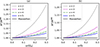 |
Fig. 6. Ratio of the Kappa and Maxwellian ponderomotive magnetic moment Mκ/MMb (a) for electron cyclotron waves as a function of ω/|Ωe| with βe = 0.1 and (b) for ion cyclotron waves as a function of ω/Ωi with βi = 0.1. |
This result is important because it tells us that even for nearly cold magnetized plasmas and for low frequencies, the effect of the kappa parameter in the ponderomotive force cannot be neglected. Therefore, it must be considered when it is applied to study wave-plasma interactions in space phenomena occurring in a large diversity of low-collision space plasma environments where the Kappa distribution is usually present, as we show in Sect. 4.
3.4. Nonlinear magnetic field perturbation due to the ponderomotive force
According to the work of Washimi and Watanabe (Washimi & Watanabe 1977), a slowly varying magnetic field B2 is generated by the ponderomotive force of an electromagnetic wave that is slowly varying in time. From the balance of the ponderomotive force with the slowly varying electromagnetic field in the electron-fluid equation of motion of an unmagnetized and homogeneous plasma, it follows that the induced magnetic field is given by
![Mathematical equation: $$ \begin{aligned} \boldsymbol{B}_2(\boldsymbol{r},t) = -\frac{c}{16\pi n_{\rm e} e \omega ^2}\frac{\partial [\omega ^2(\varepsilon - 1)]}{\partial \omega }\nabla \times (\boldsymbol{k}|\boldsymbol{E}|^2), \end{aligned} $$](/articles/aa/full_html/2024/06/aa48815-23/aa48815-23-eq46.gif) (24)
(24)
where e is the electron charge. This induced magnetization has been widely studied as a mechanism for a self-generated magnetic field. It has been analyzed for different plasma conditions, for example, relativistic electron plasmas (Qi et al. 2023) and dense plasmas (Shukla et al. 2010), due to its importance in phenomena associated with pulsar magnetospheres and compact astrophysical objects, among others. Kim and Jung calculated the Karpman–Washimi ponderomotive magnetic field for the nonthermal electrostatic case (Kim & Jung 2009), and it was also analyzed for the electromagnetic case in Espinoza-Troni et al. (2023), where it was reported that the nonthermal effect of the Kappa distributions enhances the induced magnetization due to the electromagnetic ponderomotive interactions in unmagnetized plasmas.
In this subsection, we analyze the induced Karpman–Washimi ponderomotive magnetization for nonthermal magnetized plasmas. This leads us to advance the understanding of the effect of the ponderomotive force in the nonlinear perturbation of the background magnetic field in space environments. In our work, we consider plasmas with electrons and ions, but we can still use the Karpman–Washimi induced magnetic field considering the ponderomotive force only for electrons since me/mi ≪ 1.
We note that Eq. (24) is related to the temporal term of the ponderomotive force. Therefore, by using Eq. (20) for the temporal factor of the ponderomotive force for electron cyclotron waves, we can deduce the following expression for the magnitude of the induced Karpman–Washimi magnetic field:
![Mathematical equation: $$ \begin{aligned} B_2^\kappa =&\frac{1}{16\pi }\left(\frac{\omega _{\rm pe}}{|\Omega _{\rm e}|}\right)^3\frac{1}{{ y}^{3/2}(1-{ y})^{5/2}}\nonumber \\&\times \left[1+\frac{\beta _{\rm e}}{4}\left(\frac{\kappa }{\kappa -3/2}\right)\frac{(3+4{ y}){ y}}{(1-{ y})^3}\right]\frac{|E|^2}{n_{\rm e} e L}, \end{aligned} $$](/articles/aa/full_html/2024/06/aa48815-23/aa48815-23-eq47.gif) (25)
(25)
where L is the scale length of the intensity of the field and y = ω/|Ωe|. Using this expression, we can calculate the scaled electron cyclotron frequency ωce/|Ωe| generated by the induced magnetic field:
 (26)
(26)
where ue = e|E|/meωpe is the electron quiver velocity (Kourakis & Shukla 2006). We have defined the Karpman–Washimi ponderomotive magnetization Mp(κ, y) as in Kim & Jung (2009):
![Mathematical equation: $$ \begin{aligned} M_{\rm p}(\kappa ,{ y}) = \frac{1}{4}\frac{1}{{ y}^{3/2}(1-{ y})^{5/2}}\left[1+\frac{\beta _{\rm e}}{4}\left(\frac{\kappa }{\kappa -3/2}\right)\frac{(3+4{ y}){ y}}{(1-{ y})^3}\right]\cdot \end{aligned} $$](/articles/aa/full_html/2024/06/aa48815-23/aa48815-23-eq49.gif) (27)
(27)
One can notice that this term has the same form and qualitative behavior as the temporal term of the ponderomotive force for electron cyclotron waves in Eq. (20). Therefore, the induced magnetization would increase with the kappa parameter. Hence, the nonthermal effect of the Kappa distributions enhances the induced magnetization due to the electromagnetic ponderomotive interactions in magnetized plasmas with parallel propagation. It also has a minimum for a certain value of the frequency. We note that for our deduction to be valid, we must have ωce/|Ωe|≪1, as this expression is then valid for wave amplitudes with a slow spatial variation that satisfies  . In case this condition is not satisfied, we would have to extend the Karpman–Washimi formalism for a nonperturbative ponderomotive force deduction.
In the nonrelativistic limit, we can calculate the total radiated power P average in one period produced by the gyromotion of the charges by the induced Karpman–Washimi magnetic field (Na & Jung 2009). Using the Larmor formula (Jackson 1975), this calculation is  , where rL is the Larmor radius. Because the induced magnetization increases with the decrease of the spectral index, it is expected that the nonthermal effect enhances the total energy radiated in the magnetized nonthermal plasmas. This result serves as a diagnostic tool for nonthermal magnetized space plasmas.
4. Ponderomotive force in nonthermal plasmas for different space conditions
To contextualize and specify our results, we have calculated the relative difference between Kappa and Maxwellian ponderomotive force factors for different space environments due to electron cyclotron waves. These calculations were made in a range of typical values of the plasma parameters for each space environment and for frequencies considered to be low when compared with the electron gyrofrequency with ω/|Ωe| = 0.1, for which our approximation ceases to be valid for β > 0.7. These results are displayed in Table 2 and shown graphically in Fig. 7. The values of the plasma beta and the ratio between the plasma frequency and gyrofrequency were calculated using the observations of the plasma electron density, temperature, and the strength of the background magnetic field analyzed in the references mentioned in the table. It is worth noting that these values are a rough estimation based on the observational articles given in the table. For the environments where the plasma beta can be larger than 0.7, we evaluated the relative difference of the ponderomotive force terms up to this value to be coherent with our approximation. Although these results are a general estimation and strongly depend on space weather conditions, they serve to give us a concrete idea of the impact of the nonthermal effects in the ponderomotive force and its wave-particle phenomena associated with it in a wide variety of space environments.
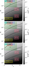 |
Fig. 7. Relative difference of the different terms of the ponderomotive force between the Kappa and Maxwellian case as a function of βe and κ. The ordinate axis and the color bar are in the logarithmic scale in base 10, and the abscissa axis is in the logarithmic scale in base 2. The abbreviations are explained in Table 2. |
Evaluation of the different terms of the ponderomotive force and the induced Karpman–Washimi magnetic field B2.
In Fig. 7, we show the effect of the Kappa distribution in the three terms of the ponderomotive force analyzed before. In the figure, one can see that this effect can be very significant for the solar wind, the magnetosheath, the plasma sheet, and the polar cusp in the presence of interplanetary (IP) shocks. Indeed, the relative difference between the Kappa and Maxwellian case is on the order of 10−2 or 10−1. In the solar wind between 0.25 AU and 0.1 AU, where we have low values of the kappa parameter between 2 and 6, we have that the ponderomotive force can be 18%, 23%, and 38% larger for the Kappa distribution case for the spatial ponderomotive term, the temporal ponderomotive term, and the ponderomotive magnetic moment, respectively. Therefore, in the near-Earth solar wind at 1 AU, the MMP term of the ponderomotive force, which will accelerate the plasma in the decreasing direction of the magnetic field strength along the interplanetary magnetic field (IMF) lines could be 38% larger for values of the frequency far from the resonances. Nevertheless, it can have plasma beta values larger than 1. In such cases, we would have to relax our approximation to evaluate the ponderomotive force. In the case of the polar cusp, we have evaluated the ponderomotive force relative differences in the occurrence of an IP shock. The shocks are associated with diamagnetic cavities (DMC) caused by the increase of plasma density and pressure as a result of the magnetosheath plasma accumulation in the cusp region, which is usually filled with energetic particles, according to analysis in Ren et al. (2023), where (among other theories) it has been proposed that the source of the energetic particles are due to wave-particle interaction mechanisms. This environment is also interesting because, as we have said before, in the polar cusps region the MMP ponderomotive force term is responsible for the acceleration and escape of ions along the open magnetic field lines, which is known as polar wind (Li & Temerin 1993; Miller et al. 1995; Guglielmi & Lundin 2001; Guglielmi 2007). Our results in Table 2 show that for this environment where the kappa parameter can have values of around 2, the absolute value of the relative difference of the ponderomotive force under the beta range of our approximation can be 18%, 23%, and 38% for the spatial, temporal, and magnetic moment terms. These results tell us that it is essential to consider the nonthermal effects of the ponderomotive force when studying these phenomena.
For other space environments such as the coronal loops in the solar corona, the magnetotail lobes (for distances relative to Earth larger than 40 Re), and the magnetopause, where the magnetic pressure is very low in comparison to the plasma pressure, the nonthermal effect is negligible, for which we have a relative difference of the ponderomotive force terms on the order of 10−4 or even 10−5. Hence, in these environments under typical conditions, the Maxwellian ponderomotive force terms can be used without issue unless we approach the resonances. Nevertheless, for the near magnetotail (between 7 Re and 20 Re), where the temperature is higher than for larger distances and therefore the plasma beta is greater than 1, we would have to extend our results, but our analysis in the sections above suggests that the nonthermal effect may have a significant impact. The same can be said for the inner heliosheath and the ring current.
On the other hand, the nonthermal effect of the nonlinear perturbed magnetic field due to the ponderomotive force would be relevant for low-temperature plasmas in the same space environments as the temporal term (see Table 2), as can be the case for the solar wind and the magnetosheath where we found that the Karpman–Washimi magnetization can be 23% and 11% larger, respectively, for the Kappa distribution than in the Maxwellian case. Therefore this nonthermal correction could be relevant to the study of the perturbation of the ponderomotive force in the interplanetary magnetic field. Indeed, it has been proposed that the ponderomotive force acts as part of a mechanism in the generation of magnetic holes observed in the solar wind (Tsurutani et al. 2002, 2005; Dasgupta et al. 2003).
It is worth noting that we are considering frequencies far from the resonances to have an accurate approximation. Nevertheless, due to the above analysis, we know that the nonthermal effect is enhanced with the frequency. Therefore, for larger frequencies, we expect that the nonthermal effects would be even more significant.
5. Conclusions
We have analyzed the consequences of considering the nonthermal effect of magnetized plasmas due to electron and ion cyclotron wave propagation, giving a detailed comparison of the different terms that make up this nonlinear force. We have also obtained an expression for the spatial and temporal terms of the ponderomotive force, its magnetic moment, and the nonlinear background magnetic field perturbation for low-temperature plasmas, which can be useful for Kappa-distributed plasmas if not also for ponderomotive phenomena occurring in a magnetized plasma with a finite temperature.
In particular, we have shown that the magnitude of the spatial term of the ponderomotive force is significantly larger for nonthermal magnetized plasmas than for Maxwellian plasmas, having a relative difference of 10−1 for the electron cyclotron waves with ωpe/|Ωe|∼101 and ion cyclotron waves with c/cA ∼ 104 and β = 0.1. Also, for the spatial term of the ponderomotive force, the nonthermal effect increases with the plasma beta for low-temperature plasmas. The same characteristics were found for the temporal factor of the ponderomotive force. We also know that the temporal factor of the ponderomotive force is responsible for the generation of a slowly varying magnetic field in the ponderomotive interaction between the electromagnetic waves and the plasma, which acts as a nonlinear perturbation of the background magnetic field. We have shown that the effect of the Kappa distribution in the nonlinear background magnetic field perturbation can be very significant. The induced magnetization can even be 25% larger than for Maxwellian plasmas for overdense plasmas in our low beta approximation for βe = 0.1, κ = 2, and ω/|Ωe| = 0.3. Also, we have shown that the ponderomotive magnetic moment responsible for the MMP force is enhanced for nonthermal plasmas in our low-temperature approximation far from resonances.
In summary, we have demonstrated that for all terms of the ponderomotive force, the effect of the Kappa distribution characterizing a magnetized plasma cannot be neglected. Indeed, even for near cold magnetized plasmas and wave frequency far from the resonance with plasma beta on the order of ∼0.1 and ω/Ω ∼ 0.3, we have shown that the nonthermal effect is very significant. Hence, our results show that the effect of the kappa parameter must be considered in ponderomotive phenomena related to nonthermal magnetized plasmas, which are commonly the characteristics of the plasma in space environments.
Indeed in Sect. 4, we evaluated the effect of the Kappa distribution in the ponderomotive force for different space environments, from which we can conclude that it is essential to consider the nonthermal effects of the ponderomotive force when studying related phenomena in such regions as the solar wind, the magnetosheath, the plasma sheet, and the polar cusp, where we can also use our approximation. For other given space conditions, for example in the ring current, the inner heliosheath, and the near magnetotail, we would have to extend our results for larger values of the plasma beta.
In addition, the analysis given in this research serves as a solid base from which to extend the study of the nonthermal effects in the ponderomotive force to other modes of propagation for magnetized plasmas, such as waves propagating obliquely to the magnetic field. Moreover, this work is useful as a starting point from which to include the effect of the Kappa distribution in some ponderomotive phenomena in space physics. The forces analyzed in this work appear in a lot of phenomena that occur due to the interaction of ion cyclotron or electron cyclotron waves with the plasma, as is the case for the acceleration of ions in the polar cusp, auroral density cavities, the penetration of solar wind in the magnetosphere, or the electromagnetic ULF waves in the terrestrial magnetosphere (Nekrasov & Feygin 2005; Lundin & Guglielmi 2007).
The results of this work can be useful in the study of the dynamics of the temperature anisotropy of electrons or ions characterized by suprathermal populations interacting with wave instabilities. Indeed, some space physics phenomena, such as magnetic holes, are correlated with temperature anisotropies (possibly) due to the acceleration resulting from the ponderomotive force (Tsurutani et al. 2002). Hence, it could be interesting to study how the ponderomotive force, when enhanced by nonthermal effects (as shown in our results), is correlated with the mechanism that deepens the relaxation of anisotropy due to suprathermal populations in the solar wind, as shown by Lazar et al. (2022). Therefore, the applications of this study can contribute to gaining a better understanding of the dynamics of space plasma physics.
Acknowledgments
J.E.-T. acknowledges the support of ANID, Chile through National Doctoral Scholarship No. 21231291. F.A.A. thanks to FONDECYT grant No. 1230094 that partially supported this work. P.S.M. thanks the support of the Research Vice-rectory of the University of Chile (VID) through grant ENL08/23.
References
- Allan, W. 1992, J. Geophys. Res. Space Phys., 97, 8483 [NASA ADS] [CrossRef] [Google Scholar]
- Bale, S. D., Goetz, K., Harvey, P. R., et al. 2016, Space Sci. Rev., 204, 49 [Google Scholar]
- Bittencourt, J. A. 2010, Fundamentals of Plasma Physics (New York: Springer) [Google Scholar]
- Bourouaine, S., Alexandrova, O., Marsch, E., & Maksimovic, M. 2012, ApJ, 749, 102 [Google Scholar]
- Brooks, D. H., Warren, H. P., & Landi, E. 2021, ApJ, 915, L24 [NASA ADS] [CrossRef] [Google Scholar]
- Burlaga, L. F., Ness, N. F., & Acuna, M. H. 2006, ApJ, 642, 584 [NASA ADS] [CrossRef] [Google Scholar]
- Chen, F. 1984, Introduction to Plasma Physics and Controlled Fusion (New York: Plenum Press) [CrossRef] [Google Scholar]
- Chen, J. 1992, J. Geophys. Res., 97, 15011 [NASA ADS] [CrossRef] [Google Scholar]
- Dasgupta, B., Tsurutani, B. T., & Janaki, M. S. 2003, Geophys. Res. Lett., 30, 017385 [CrossRef] [Google Scholar]
- Davis, S., Avaria, G., Bora, B., et al. 2019, Phys. Rev. E, 100, 023205 [NASA ADS] [CrossRef] [Google Scholar]
- Di Matteo, S., Villante, U., Viall, N., Kepko, L., & Wallace, S. 2022, J. Geophys. Res. Space Phys., 127, e30144 [NASA ADS] [CrossRef] [Google Scholar]
- Drake, J. F. 1974, Phys. Fluids, 17, 778 [NASA ADS] [CrossRef] [Google Scholar]
- Eliasson, B., & Shukla, P. 2006, Phys. Rep., 422, 225 [NASA ADS] [CrossRef] [Google Scholar]
- Espinoza, C. M., Stepanova, M., Moya, P. S., Antonova, E. E., & Valdivia, J. A. 2018, Geophys. Res. Lett., 45, 6362 [CrossRef] [Google Scholar]
- Espinoza-Troni, J., Asenjo, F. A., & Moya, P. S. 2023, Plasma Phys. Control. Fusion, 65, 065008 [CrossRef] [Google Scholar]
- Eyelade, A. V., Stepanova, M., Espinoza, C. M., & Moya, P. S. 2021, ApJS, 253, 34 [NASA ADS] [CrossRef] [Google Scholar]
- Fitzpatrick, R. 2015, Plasma Physics: An Introduction (CRC Press, Taylor& Francis Group) [Google Scholar]
- Gravanis, E., Akylas, E., & Livadiotis, G. 2020, Europhys. Lett., 130, 30005 [NASA ADS] [CrossRef] [Google Scholar]
- Guglielmi, A. V. 2007, Phys. Uspekhi, 50, 1197 [NASA ADS] [CrossRef] [Google Scholar]
- Guglielmi, A. V., & Feygin, F. Z. 2018, Izv. Phys. Solid Earth, 54, 712 [NASA ADS] [CrossRef] [Google Scholar]
- Guglielmi, A., & Feygin, F. 2023, Solar-Terr. Phys., 9, 25 [NASA ADS] [Google Scholar]
- Guglielmi, A., & Lundin, R. 2001, J. Geophys. Res. Space Phys., 106, 13219 [NASA ADS] [CrossRef] [Google Scholar]
- Guglielmi, A., Hayashi, K., Lundin, R., & Potapov, A. 1999, Earth Planets Space, 51, 1297 [Google Scholar]
- Gupta, N., Kumar, S., & Bhardwaj, S. B. 2022, J. Opt., 51, 819 [CrossRef] [Google Scholar]
- Hau, L.-N., Fu, W.-Z., & Chuang, S.-H. 2009, Phys. Plasmas, 16, 094702 [NASA ADS] [CrossRef] [Google Scholar]
- Hellberg, M. A., & Mace, R. L. 2002, Phys. Plasmas, 9, 1495 [NASA ADS] [CrossRef] [Google Scholar]
- Hellberg, M. A., Mace, R. L., Baluku, T. K., Kourakis, I., & Saini, N. S. 2009, Phys. Plasmas, 16, 094701 [CrossRef] [Google Scholar]
- Hora, H. 2007, Laser Part. Beams, 25, 37 [NASA ADS] [CrossRef] [Google Scholar]
- Hora, H. 2016, Laser Plasma Physics: Forces and the Nonlinearity Principle (Bellingham: SPIE Press) [CrossRef] [Google Scholar]
- Hora, H., Miley, G., Lalousis, P., et al. 2014, IEEE Trans. Plasma Sci., 42, 640 [CrossRef] [Google Scholar]
- Hughes, W. J. 2013, Solar Wind Sources of Magnetospheric Ultra-Low-Frequency Waves, 1 [Google Scholar]
- Jackson, J. D. 1975, Classical Electrodynamics, 2nd edn. (New York: Wiley) [Google Scholar]
- Jamil, M., Rasheed, A., Usman, M., et al. 2019, Phys. Plasmas, 26, 092110 [NASA ADS] [CrossRef] [Google Scholar]
- Kamide, Y., & Chian, A. 2007, Nonlinear Processes in Space Plasmas (Berlin, Heidelberg: Springer-Verlag), 311 [Google Scholar]
- Karpman, V. I., & Shagalov, A. G. 1982, J. Plasma Phys., 27, 215 [NASA ADS] [CrossRef] [Google Scholar]
- Karpman, V. I., & Washimi, H. 1977, J. Plasma Phys., 18, 173 [NASA ADS] [CrossRef] [Google Scholar]
- Kentwell, G., & Jones, D. 1987, Phys. Rep., 145, 319 [CrossRef] [Google Scholar]
- Kim, H.-M., & Jung, Y.-D. 2009, Phys. Plasmas, 16, 114504 [NASA ADS] [CrossRef] [Google Scholar]
- Kim, K.-H., Kim, G.-J., & Kwon, H.-J. 2018, Earth Planets Space, 70, 174 [NASA ADS] [CrossRef] [Google Scholar]
- Kirpichev, I. P., Antonova, E. E., Stepanova, M., et al. 2021, J. Geophys. Res. Space Phys., 126, e2021JA029409 [Google Scholar]
- Kletzing, C. A. 2003, J. Geophys. Res., 108, 1143 [NASA ADS] [Google Scholar]
- Kourakis, I., & Shukla, P. K. 2006, Phys. Scr., 74, 422 [NASA ADS] [CrossRef] [Google Scholar]
- Kourakis, I., Sultana, S., & Hellberg, M. A. 2012, Plasma Phys. Control. Fusion, 54, 124001 [NASA ADS] [CrossRef] [Google Scholar]
- Krall, N. A., & Trivelpiece, A. W. 1986, Principles of Plasma Physics (Berkeley: San Francisco Press) [Google Scholar]
- Lakhina, G. S. 1990, Astrophys. Space Sci., 165, 153 [CrossRef] [Google Scholar]
- Laming, J. M. 2004, ApJ, 614, 1063 [Google Scholar]
- Laming, J. M. 2015, Liv. Rev. Sol. Phys., 12, 1 [CrossRef] [Google Scholar]
- Lazar, M., & Fichtner, H. 2021, Kappa Distributions: From Observational Evidences via Controversial Predictions to a Consistent Theory of Nonequilibrium Plasmas (Cham: Springer International Publishing) [CrossRef] [Google Scholar]
- Lazar, M., Fichtner, H., & Yoon, P. 2016, A&A, 589, A39 [NASA ADS] [CrossRef] [EDP Sciences] [Google Scholar]
- Lazar, M., Kourakis, I., Poedts, S., & Fichtner, H. 2018, Planet. Space Sci., 156, 130 [NASA ADS] [CrossRef] [Google Scholar]
- Lazar, M., López, R. A., Shaaban, S. M., et al. 2022, Front. Astron. Space Sci., 8, 19 [CrossRef] [Google Scholar]
- Lazar, M., López, R. A., Poedts, S., & Shaaban, S. M. 2023, Phys. Plasmas, 30, 082106 [NASA ADS] [CrossRef] [Google Scholar]
- Li, X., & Temerin, M. 1993, Geophys. Res. Lett., 20, 13 [CrossRef] [Google Scholar]
- Livadiotis, G. 2015, J. Geophys. Res. Space Phys., 120, 1607 [NASA ADS] [CrossRef] [Google Scholar]
- Livadiotis, G., McComas, D. J., Funsten, H. O., et al. 2022, ApJS, 262, 53 [NASA ADS] [CrossRef] [Google Scholar]
- Lui, A. T., & Krimigis, S. M. 1983, Geophys. Res. Lett., 10, 13 [NASA ADS] [CrossRef] [Google Scholar]
- Lundin, R., & Guglielmi, A. 2007, Space Sci. Rev., 127, 1 [NASA ADS] [CrossRef] [Google Scholar]
- Lundin, R., & Hultqvist, B. 1989, J. Geophys. Res. Space Phys., 94, 6665 [NASA ADS] [CrossRef] [Google Scholar]
- Lundin, R., & Lidgren, H. 2022, Cosmic Implications of Ponderomotive Wave Forces (Cambridge: Cambridge Scholars Publishing) [Google Scholar]
- Lundin, R., Gustafsson, G., Eriksson, A. I., & Marklund, G. 1990, J. Geophys. Res., 95, 5905 [CrossRef] [Google Scholar]
- Mace, R. L. 1996, J. Plasma Phys., 55, 415 [NASA ADS] [CrossRef] [Google Scholar]
- Matteini, L., Hellinger, P., Landi, S., et al. 2012, Space Sci. Rev., 172, 373 [CrossRef] [Google Scholar]
- Miller, R. H., Rasmussen, C. E., Combi, M. R., Gombosi, T. I., & Winske, D. 1995, J. Geophys. Res., 100, 23901 [CrossRef] [Google Scholar]
- Moya, P. S., Lazar, M., & Poedts, S. 2020, Plasma Phys. Control. Fusion, 63, 025011 [Google Scholar]
- Na, S.-C., & Jung, Y.-D. 2009, Phys. Plasmas, 16, 074504 [NASA ADS] [CrossRef] [Google Scholar]
- Nekrasov, A. K., & Feygin, F. Z. 2005, Phys. Scr., 71, 310 [NASA ADS] [CrossRef] [Google Scholar]
- Nekrasov, A. K., & Feygin, F. Z. 2012, Astrophys. Space Sci., 341, 225 [NASA ADS] [CrossRef] [Google Scholar]
- Nekrasov, A. K., & Feygin, F. Z. 2014, Geomagnet. Aeron., 54, 23 [NASA ADS] [CrossRef] [Google Scholar]
- Nieves-Chinchilla, T., & Viñas, A. F. 2008, J. Geophys. Res. Space Phys., 113, A02105 [NASA ADS] [CrossRef] [Google Scholar]
- Ogasawara, K., Angelopoulos, V., Dayeh, M. A., et al. 2013, J. Geophys. Res. Space Phys., 118, 3126 [NASA ADS] [CrossRef] [Google Scholar]
- Phan, T. D., Paschmann, G., Baumjohann, W., Sckopke, N., & Lühr, H. 1994, J. Geophys. Res. Space Phys., 99, 121 [NASA ADS] [CrossRef] [Google Scholar]
- Pierrard, V., & Lazar, M. 2010, Sol. Phys., 267, 153 [NASA ADS] [CrossRef] [Google Scholar]
- Pisarenko, N., Budnik, E., Ermolaev, Y., et al. 2002, J. Atmos. Solar-Terr. Phys., 64, 573 [NASA ADS] [CrossRef] [Google Scholar]
- Qi, M. C., Zhan, J. Y., Liu, S. Q., & Yang, X. S. 2023, AIP Adv., 13, 015307 [NASA ADS] [CrossRef] [Google Scholar]
- Ren, J., Zong, Q., Fu, S., et al. 2023, Universe, 9, 143 [NASA ADS] [CrossRef] [Google Scholar]
- Rezapour, H., Zahed, H., & Mokhtary, P. 2018, Chin. J. Phys., 56, 1834 [NASA ADS] [CrossRef] [Google Scholar]
- Runov, A., Angelopoulos, V., Gabrielse, C., et al. 2015, J. Geophys. Res. Space Phys., 120, 4369 [NASA ADS] [CrossRef] [Google Scholar]
- Shukla, P. K., Stenflo, L., Bingham, R., & Eliasson, B. 2004, Plasma Phys. Controll. Fusion, 46, B349 [CrossRef] [Google Scholar]
- Shukla, P. K., Shukla, N., & Stenflo, L. 2010, J. Plasma Phys., 76, 25 [NASA ADS] [CrossRef] [Google Scholar]
- Slavin, J. A., Smith, E. J., Sibeck, D. G., et al. 1985, J. Geophys. Res., 90, 10875 [CrossRef] [Google Scholar]
- Stasiewicz, K., Bellan, P., Chaston, C., et al. 2000, Space Sci. Rev., 92, 423 [NASA ADS] [CrossRef] [Google Scholar]
- Stenflo, L. 1990, Phys. Scr., T30, 166 [NASA ADS] [CrossRef] [Google Scholar]
- Tsurutani, B. T., Dasgupta, B., Galvan, C., et al. 2002, Geophys. Res. Lett., 29, 86 [Google Scholar]
- Tsurutani, B. T., Lakhina, G. S., Pickett, J. S., et al. 2005, Nonlinear Process. Geophys., 12, 321 [NASA ADS] [CrossRef] [Google Scholar]
- Viñas, A. F., Mace, R. L., & Benson, R. F. 2005, J. Geophys. Res. Space Phys., 110, A06202 [Google Scholar]
- Viñas, A. F., Moya, P. S., Navarro, R. E., et al. 2015, J. Geophys. Res. Space Phys., 120, 3307 [CrossRef] [Google Scholar]
- Vocks, C., Mann, G., & Rausche, G. 2008, A&A, 480, 527 [NASA ADS] [CrossRef] [EDP Sciences] [Google Scholar]
- Washimi, H. 1989, J. Phys. Soc. Jpn., 58, 3960 [CrossRef] [Google Scholar]
- Washimi, H., & Karpman, V. I. 1976, Sov. J. Exp. Theor. Phys., 44, 528 [NASA ADS] [Google Scholar]
- Washimi, H., & Watanabe, M. 1977, J. Phys. Soc. Jpn., 42, 1081 [CrossRef] [Google Scholar]
- Wilson, L. B., III, Stevens, M. L., Kasper, J. C., et al. 2018, ApJS, 236, 41 [NASA ADS] [CrossRef] [Google Scholar]
- Wong, A. Y. 1982, Phys. Scr., T2A, 262 [NASA ADS] [CrossRef] [Google Scholar]
- Yoon, P. H. 2012, Phys. Plasmas, 19, 052301 [NASA ADS] [CrossRef] [Google Scholar]
- Yoon, P. H. 2014, J. Geophys. Res. Space Phys., 119, 7074 [NASA ADS] [CrossRef] [Google Scholar]
- Yoon, P. H. 2021, Non-equilibrium Statistical Mechanics of Electron Kappa Distribution (Cham: Springer International Publishing), 235 [Google Scholar]
- Yoon, P. H., Rhee, T., & Ryu, C.-M. 2006, J. Geophys. Res. Space Phys., 111, A09106 [NASA ADS] [Google Scholar]
Appendix A: Dispersion relation
The dielectric tensor given by Equation (2) is expressed in terms of the modified generalized plasma dispersion function ZκM(ζ). This function is defined in Hellberg & Mace (2002) as
 (A.1)
(A.1)
where Γ(x) is the gamma function.
To obtain the dispersion relation for low-temperature plasmas, we used the following asymptotic expression for ζ ≫ 1 (see Equation (55) in Hellberg & Mace 2002)
 (A.2)
(A.2)
where we have neglected the imaginary part. Considering up to the second term in this expansion and including it in the dielectric tensor given by Eq. (2), where we are considering that (ω ± Ωs)/kαs ≫ 1, we obtain that
 (A.3)
(A.3)
Then, considering Eq. (A.3) in Eq. (3), the approximated expression for the dispersion relation is given by
 (A.4)
(A.4)
Appendix B: Ponderomotive force factors
Including the dielectric tensor eigenvalue of the Equation (7) in Equation (14), we can deduce the factor  that accompanies the spatial variation in the ponderomotive force for the Kappa distribution. For both the electron waves and ion cyclotron waves, we have that
 (B.1)
(B.1)
We have neglected the terms on the order of δ2, and we have considered that ε0 ≫ 1. Using the same procedure but considering the dielectric tensor eigenvalue of Equation (4) before including the dispersion relation given by k2c2/ω2 = ε±, we can obtain the temporal factor:
![Mathematical equation: $$ \begin{aligned} f_{\rm (t)}^\kappa =&\frac{\varepsilon _0^{1/2} \omega }{16\pi c}\frac{1}{\omega ^2}\frac{\partial \omega ^2(\varepsilon _0-1)}{\partial \omega }\nonumber \\&- \frac{\varepsilon _0^{1/2}\omega }{16\pi c}\left(\frac{\kappa }{\kappa -3/2}\right)\left[\frac{\delta }{2}\frac{1}{\omega ^2}\frac{\partial \omega ^2 (\varepsilon _0 - 1)}{\partial \omega } + \varepsilon _0 \frac{\partial \delta }{\partial \omega }\right]. \end{aligned} $$](/articles/aa/full_html/2024/06/aa48815-23/aa48815-23-eq61.gif) (B.2)
(B.2)
Using these equations, we can obtain the ponderomotive force factors for electron and ion cyclotron waves.
All Tables
Maximum value of the electron plasma beta βmax that accomplishes the condition ζ−4 < 0.01 for different values of the scaled wavenumber x for electron cyclotron waves.
Evaluation of the different terms of the ponderomotive force and the induced Karpman–Washimi magnetic field B2.
All Figures
|
Fig. 1. Solution for the dispersion relation for right-handed electron cyclotron waves for y = ω/|Ωe| as a function of x = kc/ωpe with ωpe/|Ωe| = 30 for different values of κ, with (a) βe = 0.05, (b) βe = 0.1, and (c) βe = 0.5. |
| In the text | |
|
Fig. 2. Relative difference of the Kappa and Maxwellian scaled frequencies as a function of the scaled wavenumber for different values of the parameter Kappa (a) for electron cyclotron waves with βe = 0.1 and ωpe/|Ωe| = 30 and (b) for ion cyclotron waves with βi = 0.1 and cA/c = 10−3. |
| In the text | |
|
Fig. 3. Solution for the dispersion relation for left-handed ion cyclotron waves for y = ω/Ωi as a function of x = kc/ωpi, with c/cA = 102, for different values of κ with (a) βi = 0.05, (b) βi = 0.1, and (c) βi = 0.5. |
| In the text | |
|
Fig. 4. Ratio of the Kappa and Maxwellian ponderomotive spatial factor |
| In the text | |
|
Fig. 5. Ratio of the Kappa and Maxwellian ponderomotive temporal factor |
| In the text | |
|
Fig. 6. Ratio of the Kappa and Maxwellian ponderomotive magnetic moment Mκ/MMb (a) for electron cyclotron waves as a function of ω/|Ωe| with βe = 0.1 and (b) for ion cyclotron waves as a function of ω/Ωi with βi = 0.1. |
| In the text | |
|
Fig. 7. Relative difference of the different terms of the ponderomotive force between the Kappa and Maxwellian case as a function of βe and κ. The ordinate axis and the color bar are in the logarithmic scale in base 10, and the abscissa axis is in the logarithmic scale in base 2. The abbreviations are explained in Table 2. |
| In the text | |
Current usage metrics show cumulative count of Article Views (full-text article views including HTML views, PDF and ePub downloads, according to the available data) and Abstracts Views on Vision4Press platform.
Data correspond to usage on the plateform after 2015. The current usage metrics is available 48-96 hours after online publication and is updated daily on week days.
Initial download of the metrics may take a while.