| Issue |
A&A
Volume 683, March 2024
|
|
|---|---|---|
| Article Number | A188 | |
| Number of page(s) | 9 | |
| Section | Atomic, molecular, and nuclear data | |
| DOI | https://doi.org/10.1051/0004-6361/202348711 | |
| Published online | 19 March 2024 | |
New theoretical study of potassium perturbed by He and a comparison to laboratory spectra★
1
GEPI, Observatoire de Paris, PSL Research University, UMR 8111, CNRS,
Sorbonne Paris Cité, 61 Avenue de l’Observatoire,
75014
Paris,
France
e-mail: This email address is being protected from spambots. You need JavaScript enabled to view it.
2
Institut d’Astrophysique de Paris, UMR7095, CNRS, Université Paris VI,
98bis Boulevard Arago,
75014
Paris,
France
3
Department of Physics and Astronomy, University of Louisville,
Louisville,
Kentucky
40292,
USA
4
U.S. Army DEVCOM, Aviation and Missile Center,
Redstone Arsenal,
AL
35898,
USA
Received:
22
November
2023
Accepted:
20
December
2023
Abstract
The visible and near-infrared spectra of late L- and T-type dwarf stars are dominated in large part by the resonance lines of neutral Na and K. It is the collision broadening of these atomic lines by H2 and He in the stellar atmosphere that determines the continuum from below 0.5 µm to above 0.9 µm in the spectrum. Their line profiles can be detected as far as 3000 cm−1 from the line center in T dwarfs and consequently an accurate and detailed determination of the complete profile, including the extreme far wing, is required to model the contribution of these strong alkali resonance lines to brown dwarf spectra. We report on our new calculations of unified line profiles of K perturbed by He using ab initio potential data for the conditions prevailing in cool substellar brown dwarfs and hot dense planetary atmospheres with temperatures from Teff = 500 to 3000 K. For such objects with atmospheres of H2 and He, conventional laboratory absorption spectroscopy can be used to examine the line wings and test the line shape theories and molecular potentials. We find that an analytical Lorentzian profile is useful for a few cm−1 from the line center, but not in the line wings, where the radiative transfer is a consequence of the K–He radiative collisions that are sensitive to the interaction potentials. Tables of the K–He absorption coefficients of the resonance lines allow accurate model atmospheres and synthetic spectra. For this purpose, we present new opacities from comprehensive line shape theory incorporating accurate ab initio potentials. Use of these new tables for the modeling of emergent spectra will be an improvement over previous line shape approximations based on incomplete or inaccurate potentials. We also present Lorentzian impact parameters obtained in the semi-classical and quantum theory for the K 4s − 4p resonance line centered at 0.77 µm specifically for the line core regime.
Key words: atomic data / atomic processes / line: formation / molecular data / opacity / brown dwarfs
K–He opacity tables for the D1 and D2 components of the resonance line are available at the CDS via anonymous ftp to cdsarc.cds.unistra.fr (130.79.120.5) or via https://cdsarc.cds.unistra.fr/viz-bin/cat/J/A+A/683/A188
© The Authors 2024
 Open Access article, published by EDP Sciences, under the terms of the Creative Commons Attribution License (https://creativecommons.org/licenses/by/4.0), which permits unrestricted use, distribution, and reproduction in any medium, provided the original work is properly cited.
This article is published in open access under the Subscribe to Open model. This email address is being protected from spambots. You need JavaScript enabled to view it. to support open access publication.
1 Introduction
In earlier phases of the evolution of a brown dwarf star, most refractory metals have condensed to grains that have settled below their now fully radiative photosphere. The alkali elements bind less easily to molecules or grains, and their resonance transitions remain the last sources of optical opacity. The importance of the far wings of the potassium doublet, centered on 0.77 μm in the spectra of methane brown dwarfs, has been demonstrated by Burrows et al. (2000). The interatomic interactions of the low-lying states of the alkali atom with molecular hydrogen and helium are the main physical quantities needed for a good understanding of collisional processes. Calculations of Allard et al. (2001) included Lorentzian profiles using the van der Waals damping constant to generate atmosphere models of brown dwarfs that underestimated the observed line strength out to 0.9 μm for the K lines but produced too strong absorption farther from the core. This motivated Burrows et al. (2002) to modify Lorentzian profiles and to introduce cutoffs and other parameters that lack theoretical foundation. Now that theoretical potentials for the binary interactions of alkalies perturbed by He and H2 may be computed with high accuracy, the solution to the radiative collision problem may be founded on an appropriate theoretical framework for the line shape from first principles.
A subsequent improvement by Burrows & Volobuyev (2003) used multiconfiguration self-consistent field Hartree-Fock potentials in the Szudy & Baylis (1975, 1996) line shape approximation, and in Allard et al. (2003) we presented absorption profiles of sodium and potassium perturbed by He and H2 calculated in a semi-classical (SC) unified line shape theory (Allard et al. 1999) using pseudo-potentials of Pascale (1983) and Rossi & Pascale (1985) for, respectively, alkali–He and alkali–H2 interactions. These line profiles were included in model atmospheres and synthetic spectra using the (Allard et al. 2001) stellar atmosphere program PHOENIX. The results were compared to previous models in Fig. 4 of Allard et al. (2003), where the observed spectrum of the methane brown dwarf Gliese 229 was plotted for comparison. The new profiles exhibited significantly more opacity within the first 1200 Å from the line center and less opacity further out in the red wings, as was found in the observed spectra. The optical pseudo-continuum was therefore depressed, while raised at the flux maximum near 1.1 μm compared to a model based on the van der Waals approximation. The detectability of a K–H2 line satellite was predicted as well.
In a continuation of Allard et al. (2023), one goal of this paper is to update K–He opacity tables and line parameters of the resonance line (Allard et al. 2007b) previously based on the use of the pseudo-potentials of Pascale (1983). For this purpose, the Na and K line profiles perturbed by helium need to be calculated using up-to-date molecular data that affect the blue line wing satellite frequency; that is, the Na–He line satellite on the short wavelength side of the line core is closer to the unperturbed line center than was obtained with Pascale (1983) (see Fig. 4 of Allard et al. 2023). Previous opacity tables were constructed that enabled the computation of line profiles for the D1 and D2 lines of Na and K broadened by collisions with He up to nHe=1019 cm−3. New opacity tables of Na–He are now archived at the CDS and are the basis of line profiles for the D1 and D2 components to nHe = 1021 cm−3 from Teff = 150−2500 K and to nHe = 1022 cm−3 from Teff = 3000−10000 K. Accurate pressure-broadened profiles that are valid at very high densities of He are required for use in spectral models of cool white dwarf stars (Blouin et al. 2019). New K–H2 (Allard et al. 2016) and Na–H2 (Allard et al. 2019) tables that reach higher densities than nH2 = 1019 cm−3 are valuable and are now used in many studies of brown dwarfs (e.g., Burningham et al. 2017; Oreshenko et al. 2020; Lacy & Burrows 2023) and exoplanets (e.g., Phillips et al. 2020; Hou Yip et al. 2020; Gonzales et al. 2021; Chubb et al. 2021; Nikolov et al. 2022; Samra et al. 2023). Laboratory experiments serve to test and refine the theoretical models, the weak point of which is the knowledge of the interaction potential for the perturbing He atom or molecular hydrogen with the alkalies. Here we adopt a combination of the ab initio potentials of Santra & Kirby (2005) and Nakayama & Yamashita (2001) (Sect. 2.1) and the dipole moments of Santra & Kirby (2005) for the resonance line. In Sect. 2.2 we illustrate the evolution of the absorption spectra of K–He collisional profiles for the densities and temperatures prevailing in the atmospheres of brown dwarf stars. These calculations span the range Teff = 500−3000 K and take into account the spin-orbit coupling as described by Allard & Spiegelman (2006). Spectroscopic measurement of the far line wing is a sensitive tool for examining potentials (Sect. 2.3). The K–H2 laboratory results reported in Allard et al. (2016) confirm that the identification of a brown dwarf spectral feature previously interpreted as CaH absorption is the line satellite of K perturbed by H2. An additional contribution from the K–He opacity may improve the agreement with the observation (Sect. 2.4). We compare the obtained spectral line parameters to those calculated using the quantum Baranger-Lindholm theory (Sect. 3). Impact broadening and shift, and satellites in the line wings due to binary collisions, are all sensitive to different details of the atomic and molecular interactions, as is shown in the appendices.
2 K–He unified profiles
In our work, a unified line shape theory and a set of atomic interaction potential energies were used to model the entire line profile from the impact-broadened line center to the far wing. Complete details and the derivation of the theory are given in Allard et al. (1999). A rapid account of the theory is given in a recent paper (Allard et al. 2023).
Prominent line satellites with He and H2 are excellent tests of line shape theory and atomic interaction potentials (Allard et al. 2012, 2016, 2019, 2023).
2.1 K–He diatomic potentials
The theoretical potentials for the binary interactions of alkali atoms perturbed by He were computed for the lower states to an accuracy suitable for line shape calculations by Pascale (1983). They were obtained by using l-dependent pseudo-potentials with parameters constrained by spectroscopic and scattering data. These potentials were used for the resonance lines of Na, K (Allard et al. 2003), Li (Allard et al. 2005), Rb, and Cs (Allard & Spiegelman 2006).
However, with vast improvements in computational power and refinements in code and methodology, significant progress in the ab initio potentials of the resonance line of K has been been achieved, as was reported by Nakayama & Yamashita (2001), Enomoto et al. (2004), Santra & Kirby (2005), Mullamphy et al. (2007), Boutarfa et al. (2012), and Blank et al. (2012). In the present work, we used the K–He ab initio potentials of Santra & Kirby (2005) at a short internuclear distance and those of Nakayama & Yamashita (2001) elsewhere. Figures 1–2 show our adopted potentials (black line) compared to the potential data of Nakayama & Yamashita (2001) (dashed green line) and to those of Santra & Kirby (2005) (dotted red line). In Fig. 2 we also compare our potentials with those computed by Pascale (1983) (dashed blue line). The main difference occurs at short distances in the repulsive wall of the B potential of Pascale (1983) that is less repulsive. This difference affects the blue satellite position, as is described in the next section.
Laboratory experiments reported in Kielkopf et al. (2012) and Kielkopf et al. (2017) served to test the theoretical line shape calculations based on ab initio potentials of Santra & Kirby (2005) to determine the blue wing of the potassium resonance lines broadened by He. The improvement over our previous work consists of more accurate intermediate and long-range parts of the K–He potential curves achieved by Nakayama & Yamashita (2001), which enables a better determination of the line parameters of the two components of the doublet (see Sect. 3).
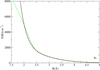 |
Fig. 1 Potential curve for the 4s X 2∑1/2 state of K–He used in this work (black line). The K–He potentials of Nakayama & Yamashita (2001) (dashed green line) and Santra & Kirby (2005) (dotted red line) are superimposed. |
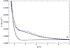 |
Fig. 2 Potential curves for the 4p A Π and 4p B 2Σ states of the K–He molecule for ab initio potentials of Nakayama & Yamashita (2001) (dashed green line) are compared to potentials of Santra & Kirby (2005) (dotted red line), pseudo-potentials of Pascale (1983) for the B 2Σ state (dashed blue line), and the adopted potentials (black line). |
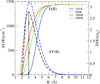 |
Fig. 3 ∆V(R) (dashed black line) compared to Pascale (1983) (dashed blue line) and the temperature dependence of the modulated dipole, D(R), (solid line) corresponding to the 4s X → 4p B P3/2 transition of the K D2 line. |
2.2 Quasi-molecular absorption in the blue wing
The line wing generally does not decrease monotonically with increasing frequency separation from the line center. Its shape, for an atom in the presence of other atoms, is sensitive to the difference between the initial and final state interaction potentials. When this difference, for a given transition, goes through an extremum, a wider range of interatomic distances contribute to the same spectral frequency, resulting in an enhancement, or satellite, in the line wing. Satellites in alkali spectra have been known since the 1930s (Allard & Kielkopf 1982). More recently, laboratory spectra of both Na and K alkalies with H2, He, and other rare gases have been found to exhibit a systematic pattern of satellites in the blue wings. Quasi-molecular satellites are associated with each gas and their presence is predicted by line shape theory using the most accurate atomic potentials available (see Fig. 3 of Kielkopf et al. 2017). The line wing intensities are most sensitive to the values of the difference potential at relatively short internuclear distances, which is why they require the use of accurate atomic potentials. Blue satellite bands in alkali-He/H2 profiles are correlated with maxima in the excited B state potentials and can be predicted from the maxima in the difference potentials, ∆V, for the B-X transition.
In the case of K–He, the 4s 2Σ − 4p 2Σ transition goes through a maximum, ∆V, when the atoms are 3 Å apart (Fig. 3). This leads to a “blue” satellite on the short wavelength wing of the resonance doublet. The difference potential maxima, as is shown in Fig. 3, are 1480 and 1290 cm−1 for the B–X transition when using, respectively, the pseudo-potentials of Pascale (1983) and our adopted ab initio potentials. Far wings are extended to more than 2000 cm−1 from the line center when the helium density is 1020 cm−3 at 3000 K. Figure A.1 shows how the unified theoretical approach is a major improvement compared to the unrealistic use of a Lorentzian so far in the wings.
Another important factor for the presence of spectral line satellites is the variation in the electric dipole transition moment during the collision, modulated by the Boltzmann factor,  . Here, Ve is the ground state potential when we consider absorption profiles, or an excited state for the calculation of a profile in emission. In Eq. (117) of Allard et al. (1999), we define
  as a modulated dipole,
![Mathematical equation: $D(R) \equiv {\mathop d\limits^ _{ee'}}[R(t)] = {d_{ee'}}[R(t)]{e^{ - {{{V_e}[R(t)]} \over {2kT}}}},$](/articles/aa/full_html/2024/03/aa48711-23/aa48711-23-eq3.png) (1)
(1)
where d(R) is the transition dipole moment of Santra & Kirby (2005). The presence of line satellite features is very sensitive to the temperature, due to the fast variation of the modulated dipole moment, D(R) (Eq. (1)), with temperature (Fig. 3). The magnitude of the dipole moment determines the relative significance these regions have within the spatial volume where collisions contribute to the line wing. However, the modulated dipole decreases significantly inside 4 Å, and the region in which the satellite would develop contributes only at elevated temperatures larger than 500 K. The behavior for Na with He is similar (Allard et al. 2023). In Fig. 4 we illustrate the evolution of the absorption cross section of the resonance line of K for a He density of 1020 cm−3 and temperatures from 150 to 3000 K, the temperatures prevailing in the atmospheres of brown dwarf stars. These potentials lead to far wing line profiles with a KHe satellite on the blue side of the D lines, and a monotonically decreasing wing on the red side (Figs. 4 and 5). When the line center is strongly saturated, these wings can become a significant source of opacity. In Figs. 4 and A.1 we highlight the region of interest near the KHe quasi-molecular satellite for comparison with previous results described in Allard et al. (2003) and calculations based on the ab initio potentials of Blank et al. (2012).
At this moderate pressure, less than 1 bar, the line profile intensities are related to the perturbations caused by a single binary collision event. The binary model, for an optically active atom in collision with one perturber, is valid for the whole profile except the central part of the line. The formation of the KHe quasi-molecule at 0.707 μm is in agreement with quantum mechanical calculations carried out by Zhu et al. (2006) and Boutarfa et al. (2012).
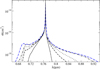 |
Fig. 4 Variation in the absorption cross section of the D2 component with temperature, (from top to bottom, T = 3000, 1000, 500, and 150 K, nHe = 1020 cm−3). The corresponding profile for T = 3000 K using the pseudo-potentials of Pascale (1983) is overplotted (dashed blue line). |
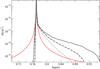 |
Fig. 5 Variation in the absorption cross section of the D1 component with temperature (from top to bottom, T = 3000, 1000, and 500 K, nHe = 1020 cm−3). |
2.3 Laboratory spectra of K perturbed by He and H2
Previous experimental spectra explored the near wing of the alkalies with rare gases, and supported the development of pseu-dopotential theories for the interactions of these complex systems (McCartan & Farr 1976; Lwin & McCartan 1978). Experiments at high pressures and room temperatures were carried out by Scheps et al. (1975) for Li–He and by York et al. (1975) for Na–He but no measurements were done for K–He. More recently, Shindo et al. (2007) reported experimental profiles for the second member of the K principle series broadened by He. At lower temperatures, experiments to determine the emission spectrum were conducted by Havey et al. (1980) for Na–He and by Enomoto et al. (2004) for Li/Na/K–He. It is a straightforward application of dispersive laboratory spectroscopy to determine the absorption spectrum of the alkalies broadened by gases, since modern detector technology enables high-precision quantitative measurements of the absorption coefficient. The spectra shown in Fig. 6 were acquired using conventional absorption spectroscopy of an alkali vapor cell in a uniformly heated oven. The measurements used a methodology that has been described previously (Kielkopf 1980, 1983). In this section, we will briefly describe the experiment design. More details were given in Allard et al. (2012). A CCD detector recorded the full spectral range in a single exposure with a 0.16 meter focal length Czerny-Turner spectrograph operated at 4 Å pixel dispersion. The alkali was introduced as 99.95% purity metal containing detectable Na, Rb, and Cs in the case of K, and as K, Rb, and Cs in the case of Na. Gases were spectroscopic-grade and trace impurities were not significant for the line broadening measurements. For Na and K with H2 and other gases, the difficulties lie primarily in handling the alkalies, and in the usual hazards of H2, but temperatures up to 1000 K and pressures up to one atmosphere are readily obtained. The laboratory spectrum of K with H2, He, and other gases also shows a systematic pattern of satellites in the blue wing (Kielkopf et al. 2017). Xe and Kr produce the strongest satellites closest to the parent line, as was expected from the longer range but weaker interactions of these noble gases. By contrast, H2 and He produce satellites farthest from the line. The absorption spectra of K with He and H2 were measured at pressures under 1 bar under controlled conditions in the laboratory to compare with the unified theory calculations and validation of ab initio potentials. In previous experimental and theoretical work on Na perturbed by H2, we also reported the Na line wings measured similarly (Allard et al. 2012). As in that work, the data we report on here are from a series of spectra taken of a K absorption cell with a uniformly heated central section, 30 cm long by 2.2 cm in diameter. Both Na and K form stable Na2 and K2 molecules that absorb in part of the region of interest. The presence of these dimers is unavoidable at the relatively low temperatures used in an absorption cell. They are apparent because the vapor pressure of the alkali is intentionally raised to make the extreme wing of the atomic line observable. We also took data with Kr buffer gas to remove this molecular background and reveal only the atomic K–He and K–H2 contributions. Spectra with Kr, and all rare gases other than He, have classically inaccessible line wing contributions to the spectral region where the singular KHe and KH2 features occur, and therefore provide an absorption coefficient only due to K2. It is straightforward then to remove this component by subtraction and leave only the coefficient of absorption due to K–He and K–H2 in the reduced experimental data. While the pseudopotentials of Rossi & Pascale (1985) overestimated the displacement of the KH2 satellite from the line, ab initio potentials described in Allard et al. (2007c) predicted a satellite that matches the observations of ϵIndi Ba more precisely (Fig. 7). The observed laboratory spectra of K with H2 and He shown in Fig. 6 agree exceptionally well with our theoretical profiles. They confirm the identification of the brown dwarf spectral feature of ϵ Indi Ba,b as being due to K–H2/He.
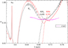 |
Fig. 6 Comparison of the theoretical blue line wings of the resonance line of K (dotted lines) with the experimental spectra (full lines). The red curve represents K–He and the black curve represents K–H2. The density of perturbers is 1019 cm−3 at 800 K. The experimental spectra show the K2 dimer absorption. Detail of the spectrum of ϵ Indi Ba shows the blue satellite of the K resonance lines (observational data of Mark McCaughrean, as was described in Allard et al. 2007a). |
2.4 Quasi-molecular absorption in T-type brown dwarfs
A broad and shallow absorption feature centered around 0.695 μm in the blue wing of the K doublet at 0.77 μm was identified by (Burgasser et al. 2003) as the CaH system. The model atmosphere and synthetic spectra of Allard et al. (2003) have shown the possible detectability of the quasi-molecular line due to K–H2 collisions. Figure 7, extracted from Allard et al. (2007a), shows a region of an exceptionally high-quality spectrum of ϵ Indi Ba,b that includes the blue wing of the K doublet. The ɛ Indi Ba,b binary system is a unique test for brown dwarf models. This spectrum illustrates how the visible spectra of brown dwarfs may be dominated by the strong absorption from two abundant alkalies, Na and K.
In Allard et al. (2007c), we have shown that ab initio K–H2 potentials systematically less repulsive than the pseudo-potentials of Rossi & Pascale (1985) enabled a KH2 quasi-molecular line satellite to be predicted. This satellite closely matches the position and shape of an observed feature in the spectrum of the Tl dwarf ɛ Indi Ba (Allard et al. 2007a).
Figure 10 of Allard et al. (2016) shows an exceptionally good match between the K–H2 experimental spectrum and the model from the unified line shape theory with the new K–H2 potentials. As was noticed in Allard et al. (2007a), the new theoretical line satellite apparently does not extend far enough to the red to reproduce the more elongated shape of the observed feature (Fig. 7). Collisions with H2 are preponderant in brown dwarf atmospheres with an effective temperature of about 1000 K, but collisions with He should be considered as well (see Fig. 8), and new K-He collisional profiles might improve the agreement with the observation of the spectrum of the T1 dwarf ɛ Indi Ba.
In the next section, we examine the dependence of the new KHe line parameters on the temperature.
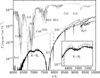 |
Fig. 7 FORS2 red optical spectrum of the T1 dwarf ɛ Indi Ba (solid), compared to synthetic spectra for a 1.3 Gyr (dashed) and 2 Gyr (dotted) model (extracted from Allard et al. 2007a). |
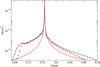 |
Fig. 8 Absorption cross section of the D2 component of the resonance lines of K perturbed by He and H2 collisions. The density of perturbers is 1020 cm−3 at 1000 K. The red curve represents K–He and the black curve represents K–H2. The Lorentzian approximation is overplotted for comparison. |
3 Line core parameters
3.1 Semi-classical calculations
The theory of spectral line shapes, especially the unified approach that we have developed and refined, makes possible models of stellar spectra that account for the centers of spectral lines and their extreme wings in one consistent treatment.
The impact theories of pressure broadening (Baranger 1958; Kolb & Griem 1958) are based on the assumption of sudden collisions (impacts) between the radiator and perturbing atoms, and are valid when frequency displacements, ∆ ω = ω − ω0, and gas densities are sufficiently small. In impact broadening, the duration of the collision is assumed to be small compared to the interval between collisions, and the results describe the line within a few line widths of the center. One outcome of our unified approach is that we may evaluate the difference between the impact limit and the general unified profile, and establish with certainty the region of validity of an assumed Lorentzian profile. In the planetary and brown dwarf upper atmospheres, the He density is of the order of 1016 cm−3 in the region of line core formation. At these sufficiently low densities of the perturbers, the symmetric center of a spectral line is Lorentzian and can be defined by two line parameters, the width and the shift of the main line. These quantities can be obtained in the impact limit (s → ∞) of the general calculation of the autocorrelation function (Eq. (121) of Allard et al. 1999). In the following discussion, we refer to this line width as measured by half the full width at half the maximum intensity – what is customarily termed HWHM.
In Allard et al. (2007b), spectral line widths of the light alkalies perturbed by He and H2 were presented for conditions prevailing in brown dwarf atmospheres. We used pseudo-potentials in a SC unified theory of the spectral line broadening (Allard et al. 1999) to compute line core parameters. For the specific study of the D1 (P1/2) and D2 (P3/2) components, we need to take the spin-orbit coupling of the alkali into account. This is done using an atom-in-molecule intermediate spin-orbit coupling scheme, analogous to the one derived by Cohen & Schneider (1974). The degeneracy is partially split by the coupling and the distinction between D1 and D2 results. We used the molecular structure calculations performed by Pascale (1983) for the adiabatic potentials of alkali–metal–He systems.
The new determinations of line width using our adopted potentials in a wide range of temperatures are presented in Fig. 9. The line widths, w (HWHM), are linearly dependent on He density, and a power law in temperature is given for the 2P1/2 component by
 (2)
(2)
and for the 2P3/2 component by
 (3)
(3)
These expressions may be used to compute the widths for temperatures of stellar atmospheres from 150 to at least 3000 K.
When it is assumed that the main interaction between two atoms is the long-range van der Waals interaction of two dipoles, the Lindholm-Foley theory gives the usual formulae for the width and shift. The van der Waals damping constant is calculated according to the impact theory of the collision broadening. In Fig. D.1, we compare our calculation of the SC KHe D1 and D2 broadening rates using two different sets of potential energy curves, our adopted potentials, and the ab initio potentials from Blank et al. (2012).
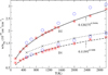 |
Fig. 9 Variation with temperature of the broadening rate (w/nHe) of the 4P3/2–4s (solid line) and 4P1/2–4s (dashed line) resonance lines of K perturbed by He collisions. A comparison is made with Pascale (1983) (blue circle) and van der Waals (dotted black line). The rates are in units of 10−20 cm−1/cm−3. |
3.2 Quantum calculations
Quantum scattering calculations of the D1 and D2 line broadening rates and shift rates were performed using the Baranger-Lindholm (BL) theory (Baranger 1958) in the manner described in our previous paper for Na-He collisions (Allard et al. 2023). Relative phase shifts between the ground and excited states are obtained from plane wave scattering calculations, using the relevant potential energy curves for fine-structure states involving the two lines. Calculations were performed over a range of temperatures, with each temperature represented by an average relative momentum,  , between radiator and perturber atoms. Partial wave expansions were used up to maximum angular momenta,
  , where 76 au is the interatomic distance over which the K-He potential is significant, for the states considered here, and where
  ranged from 2.3–12.7 au for the temperature range, 100–3000 K. Radial solutions of the Schrödinger equation were computed out to Rmax = 300 au.
Figure 10 overlays the quantum calculations of the broadening and shift rates obtained from BL theory with the rates from the SC theory. Excellent agreement between the SC and quantum calculations is seen in the range 150–1500 K. Beyond 1500 K, the quantum rates exhibit stronger coherent oscillations as a result of using the average relative momentum,  , to represent the temperature. Ideally, for a gas in thermal equilibrium, an average of the broadening and shift rates would be computed using the thermal distribution of relative momenta,
 (4)
(4)
where μ is the reduced mass of the radiator-perturber system. A set of scattering phase shifts, for l = 0−lmax, must then be computed at each k, over a fine enough mesh in k, and extended over a sufficiently large range in k in order to obtain an accurate thermal average at each temperature. While we expect that the oscillations in the BL rates will be smoothed out by performing the thermal average, we note that the broadening rates for both SC and quantum calculations, shown in Fig. 10, remain close to each other up to T = 3000 K. Thus, we expect that Eqs. (2) and (3) will also represent the broadening rates of the D1 and D2 lines from BL theory when properly averaged over the relative momentum distribution (Eq. (4)) of each temperature.
In Table 1 we compare our D1 and D2 broadening rates from BL theory, computed at 300 K, with other recently predicted rates, given in Table 4 of Ding et al. (2022). We also compare the predicted broadening rates with the recent experimental measurements of Ding et al. (2022). Our predicted broadening rates are seen to agree to better than 1% with the experimental rates given in Table 3 of Ding et al. (2022), for both D1 and D2 lines. Our BL rates at T = 300 K are also in excellent agreement with the quantum calculations of Mullamphy et al. (2007).
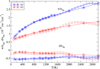 |
Fig. 10 Variation with temperature of the broadening rate (w/nHe) and shift rate (d/nHe) of the 4P3/2 −4s (blue) and 4P1/2−4s (red) resonance lines of K perturbed by He collisions. The BL theory is represented by circles and the SC theory by stars. The rates are in units of 10−20 cm−1/cm−3. |
Comparison of theoretical and experimental broadening rates, w/nHe (10−20 cm−1/cm−3), of the K resonance lines.
3.3 Contribution of the different components
In Tables B.1 and C.1 we report our computed half-width broadening and shift rates obtained in the SC theory and in the quantum calculation (BL) for the different transitions. The P1/2 line is due to a simple isolated A Π1/2 state, whereas the P3/2 line comes from the A Π3/2 and B Σ1/2 adiabatic states arising from the 3p P3/2 atomic state. The broadening of the B Σ1/2 state is most sensitive to potential at intermediate separations, where the potential starts to deviate from the long range part. This result confirms the study by Roueff & van Regemorter (1969) and Lortet & Roueff (1969) of the collisions with light atoms whose polarisability is small. It was shown by them that the width of spectral lines due to collisions with hydrogen atoms does not arise from the van der Waals dispersion forces but from a shorter-range interaction.
4 Conclusions
The optical spectra of L- and T-dwarfs exhibit a continuum dominated by the far wings of the absorption profiles of the Na 3s–3p and K 4s–4p doublets perturbed by molecular hydrogen and helium. Studies of observed L- and T-dwarf spectra by Liebert et al. (2000) and Burrows et al. (2001) showed clearly the importance of extended K line wings and pointed out the need for spectral broadening calculations more accurate than Lorentzian profiles. Understanding the shape of these lines is essential to modeling the transport of radiation from the interior. Compared to the commonly used van der Waals broadening in the impact approximation, major first improvements in the theoretical description of pressure broadening have been made by Burrows & Volobuyev (2003) and Allard et al. (2003).
All line shape characteristics depend on the accuracy of the atomic potentials and transition moments, and laboratory observations are crucial for testing the molecular data. Spectral line shapes shown here were computed in a unified theory (Allard et al. 1999) using ab initio potentials that reproduce laboratory and astrophysical data (Allard et al. 2012, 2016, 2019, 2023). We have shown that they confirm the identification of a brown dwarf spectral feature is due to line satellites of potassium perturbed by H2. This feature was previously interpreted as CaH absorption bands. An additional contribution from the new K–He opacities reported here should improve the agreement. These dwarf star spectroscopic measurements required the largest available ground-based telescopes with complex and efficient spectrographs to acquire data with an adequate signal-to-noise ratio. Consequently, examples of high-quality spectra of brown dwarfs for wavelengths below the K resonance lines are rare. Indeed, this spectral region from 0.68 to 0.74 μm is very temperature-dependent and is very constraining on atmosphere models in comparison to observations because of the overlap of the red wing of the (3s–3p) resonance line of sodium with the blue wing of the (4s–4p) resonance line of potassium (Allard et al. 2007c). The contribution of the quasi-molecular KHe absorption near 0.707 μm that we find is expected to reproduce the observations of the T-dwarf ɛ Indi Ba and similar stars in a more realistic way than previous calculations did (Allard et al. 2007a). The new opacity tables of K–He are archived at the CDS.
Appendix A Extension of the wings
For a He density lower than nHe= 1020 atoms cm−3, the core of the line is described adequately by a Lorentzian profile. This figure demonstrates that unified profiles provide more absorption close to the line core, while less far out in the red wing, compared to the use of a Lorentz profile.
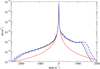 |
Fig. A.1 Absorption cross section of the K D2 component at T =3000 K, nHe=1× 1020 cm−3 (black line) compared to the Lorentzian profile (red line). The corresponding profiles for T=3000 K using the pseudo-potentials of Pascale (1983) (dashed blue line) and the ab initio potentials of Blank et al. (2012) (dotted black line) are overplotted. |
Appendix B Line broadening rate
Computed broadening rates, w/nHe (10−20 cm−1/cm−3), of K resonance lines perturbed by He collisions. Values are given from both SC and quantum (BL) calculations.
Appendix C Line shift rate
Computed shift rates, d/nHe (10−20 cm−1/cm−3), of K resonance lines perturbed by He collisions. Values are given from both SC and quantum (BL) calculations.
Appendix D Comparison of line broadening for two sets of ab initio potentials
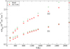 |
Fig. D.1 Variation with temperature of the broadening rate (w/nHe) of the 4P3/2-4s (blue) and 4P1/2-4s (red) resonance lines of K perturbed by He collisions. Blank et al. (2012) is shown in green and this work (SC) is shown in red. The rates are in units of 10−20 cm−1/cm−3. |
References
- Allard, N. F., & Kielkopf, J. F. 1982, Rev. Mod. Phys., 54, 1103 [Google Scholar]
- Allard, N. F., & Spiegelman, F. 2006, A&A, 452, 351 [NASA ADS] [CrossRef] [EDP Sciences] [Google Scholar]
- Allard, N. F., Royer, A., Kielkopf, J. F., & Feautrier, N. 1999, Phys. Rev. A, 60, 1021 [Google Scholar]
- Allard, F., Hauschildt, P. H., Alexander, D. R., Tamanai, A., & Schweitzer, A. 2001, ApJ, 556, 357 [Google Scholar]
- Allard, N. F., Allard, F., Hauschildt, P. H., Kielkopf, J. F., & Machin, L. 2003, A&A, 411, L473 [NASA ADS] [CrossRef] [EDP Sciences] [Google Scholar]
- Allard, N. F., Allard, F., & Kielkopf, J. F. 2005, A&A, 440, 1195 [NASA ADS] [CrossRef] [EDP Sciences] [Google Scholar]
- Allard, F., Allard, N. F., Homeier, D., et al. 2007a, A&A, 474, L21 [NASA ADS] [CrossRef] [EDP Sciences] [Google Scholar]
- Allard, N. F., Kielkopf, J. F., & Allard, F. 2007b, EPJ D, 44, 507 [Google Scholar]
- Allard, N. F., Spiegelman, F., & Kielkopf, J. F. 2007c, A&A, 465, 1085 [NASA ADS] [CrossRef] [EDP Sciences] [Google Scholar]
- Allard, N. F., Spiegelman, F., Kielkopf, J. F., Tinetti, G., & Beaulieu, J. P. 2012, A&A, 543, A159 [NASA ADS] [CrossRef] [EDP Sciences] [Google Scholar]
- Allard, N. F., Spiegelman, F., & Kielkopf, J. F. 2016, A&A, 589, A21 [NASA ADS] [CrossRef] [EDP Sciences] [Google Scholar]
- Allard, N. F., Spiegelman, F., Leininger, T., & Molliere, P. 2019, A&A, 628, A120 [NASA ADS] [CrossRef] [EDP Sciences] [Google Scholar]
- Allard, N. F., Myneni, K., Blakely, J. N., & Guillon, G. 2023, A&A, 674, A171 [NASA ADS] [CrossRef] [EDP Sciences] [Google Scholar]
- Baranger, M. 1958, Phys. Rev., 111, 481 [NASA ADS] [CrossRef] [Google Scholar]
- Blank, L., & Weeks, D. E. 2014, Phys. Rev. A, 90, 022510 [NASA ADS] [CrossRef] [Google Scholar]
- Blank, L., Weeks, D. E., & Kedziora, G. S. 2012, J. Chem. Phys., 136, 124315 [NASA ADS] [CrossRef] [Google Scholar]
- Blouin, S., Dufour, P., Allard, N. F., et al. 2019, ApJ, 872, 188 [NASA ADS] [CrossRef] [Google Scholar]
- Boutarfa, H., Alioua, K., Bouledroua, M., Allouche, A. R., & Aubert-Frécon, M. 2012, Phys. Rev. A, 86, 052504 [NASA ADS] [CrossRef] [Google Scholar]
- Burgasser, A. J., Kirkpatrick, J. D., Liebert, J., & Burrows, A. 2003, ApJ, 594, 510 [NASA ADS] [CrossRef] [Google Scholar]
- Burningham, B., Marley, M. S., Line, M. R., et al. 2017, MNRAS, 470, 1177 [NASA ADS] [CrossRef] [Google Scholar]
- Burrows, A., & Volobuyev, M. 2003, ApJ, 583, 985 [Google Scholar]
- Burrows, A., M. S. Marley, M. S., & Sharp, C. M. 2000, ApJ, 531, 438 [NASA ADS] [CrossRef] [Google Scholar]
- Burrows, A., Hubbard, W. B., Lunine, J. I., & Liebert, J. 2001, Rev. Mod. Phys., 73, 719 [Google Scholar]
- Burrows, A., Burgasser, A. J., Kirkpatrick, J. D., et al. 2002, ApJ, 573, 394 [NASA ADS] [CrossRef] [Google Scholar]
- Chubb, K. L., Rocchetto, M., Yurchenko, S. N., et al. 2021, A&A, 646, A21 [NASA ADS] [CrossRef] [EDP Sciences] [Google Scholar]
- Cohen, J. S., & Schneider, B. 1974, J. Chem. Phys., 61, 3230 [Google Scholar]
- Ding, Y., Vandervort, J. A., Freedman, R. S., et al. 2022, J. Quant. Spectrosc. Radiat. Transf., 283, 108149 [NASA ADS] [CrossRef] [Google Scholar]
- Enomoto, K., Hirano, K., Kumakura, M., Takahashi, Y., & Yabuzaki, T. 2004, Phys. Rev. A, 69, 012501 [NASA ADS] [CrossRef] [Google Scholar]
- Gonzales, E. C., Burningham, B., Faherty, J. K., et al. 2021, ApJ, 923, 19 [NASA ADS] [CrossRef] [Google Scholar]
- Havey, M. D., Frolking, S. E., & Wright, J. J. 1980, Phys. Rev. Lett., 45, 1783 [NASA ADS] [CrossRef] [Google Scholar]
- Hou Yip, K., Changeat, Q., Edwards, B., et al. 2020, Euro. Planet. Sci. Cong., 2020, 67 [Google Scholar]
- Kielkopf, J. F. 1980, J. Phys. B At. Mol. Opt. Phys., 13, 3813 [NASA ADS] [CrossRef] [Google Scholar]
- Kielkopf, J. F. 1983, J. Phys. B At. Mol. Opt. Phys., 16, 3149 [NASA ADS] [CrossRef] [Google Scholar]
- Kielkopf, J. F., Allard, N. F., & Babb, J. 2012, EAS Pub. Ser., 58, 75 [NASA ADS] [CrossRef] [EDP Sciences] [Google Scholar]
- Kielkopf, J. F., Allard, N. F., Alekseev, V. A., et al. 2017, J. Phys. Conf. Ser., 810, 012023 [NASA ADS] [CrossRef] [Google Scholar]
- Kolb, A. C., & Griem, H. 1958, Phys. Rev., 111, 514 [NASA ADS] [CrossRef] [Google Scholar]
- Lacy, B., & Burrows, A. 2023, ApJ, 950, 8 [NASA ADS] [CrossRef] [Google Scholar]
- Liebert, J., Reid, I., Burrows, A., et al. 2000, ApJ, 533, L155 [NASA ADS] [CrossRef] [Google Scholar]
- Lortet, M. C., & Roueff, E. 1969, A&A, 3, 462 [NASA ADS] [Google Scholar]
- Lwin, N., & McCartan, D. G. 1978, J. Phys. B At. Mol. Opt. Phys., 11, 3841 [NASA ADS] [CrossRef] [Google Scholar]
- McCartan, D. G., & Farr, J. M. 1976, J. Phys. B At. Mol. Opt. Phys., 9, 985 [NASA ADS] [CrossRef] [Google Scholar]
- Mullamphy, D. F. T., Peach, G., Venturi, V., Whittingham, I. B., & Gibson, S. J. 2007, J. Phys. B At. Mol. Opt. Phys., 40, 1141 [NASA ADS] [CrossRef] [Google Scholar]
- Nakayama, A., & Yamashita, K. 2001, J. Chem. Phys., 114, 780 [NASA ADS] [CrossRef] [Google Scholar]
- Nikolov, N. K., Sing, D. K., Spake, J. J., et al. 2022, MNRAS, 515, 3037 [NASA ADS] [CrossRef] [Google Scholar]
- Oreshenko, M., Kitzmann, D., Márquez-Neila, P., et al. 2020, AJ, 159, 6 [Google Scholar]
- Pascale, J. 1983, Phys. Rev. A, 28, 632 [NASA ADS] [CrossRef] [Google Scholar]
- Phillips, M. W., Tremblin, P., Baraffe, I., et al. 2020, A&A, 637, A38 [NASA ADS] [CrossRef] [EDP Sciences] [Google Scholar]
- Rossi, F., & Pascale, J. 1985, Phys. Rev. A, 32, 2657 [CrossRef] [Google Scholar]
- Roueff, E., & van Regemorter, H. 1969, A&A, 1, 69 [NASA ADS] [Google Scholar]
- Samra, D., Helling, C., Chubb, K. L., et al. 2023, A&A, 669, A142 [NASA ADS] [CrossRef] [EDP Sciences] [Google Scholar]
- Santra, R., & Kirby, K. 2005, J. Chem. Phys., 123, 214309 [NASA ADS] [CrossRef] [Google Scholar]
- Scheps, R., Ottinger, C., York, G., & Gallagher, A. 1975, J. Chem. Phys., 63, 2581 [NASA ADS] [CrossRef] [Google Scholar]
- Shindo, F., Babb, J. F., Kirby, K., & Yoshino, K. 2007, J. Phys. B At. Mol. Opt. Phys., 40, 2841 [NASA ADS] [CrossRef] [Google Scholar]
- Szudy, J., & Baylis, W. 1975, J. Quant. Spectrosc. Radiat. Transf., 15, 641 [CrossRef] [Google Scholar]
- Szudy, J., & Baylis, W. 1996, Phys. Rep., 266, 127 [NASA ADS] [CrossRef] [Google Scholar]
- York, G., Scheps, R., & Gallagher, A. 1975, J. Chem. Phys., 63, 1052 [NASA ADS] [CrossRef] [Google Scholar]
- Zhu, C., Babb, J. F., & Dalgarno, A. 2006, Phys. Rev. A, 73, 012506 [NASA ADS] [CrossRef] [Google Scholar]
All Tables
Comparison of theoretical and experimental broadening rates, w/nHe (10−20 cm−1/cm−3), of the K resonance lines.
Computed broadening rates, w/nHe (10−20 cm−1/cm−3), of K resonance lines perturbed by He collisions. Values are given from both SC and quantum (BL) calculations.
Computed shift rates, d/nHe (10−20 cm−1/cm−3), of K resonance lines perturbed by He collisions. Values are given from both SC and quantum (BL) calculations.
All Figures
|
Fig. 1 Potential curve for the 4s X 2∑1/2 state of K–He used in this work (black line). The K–He potentials of Nakayama & Yamashita (2001) (dashed green line) and Santra & Kirby (2005) (dotted red line) are superimposed. |
| In the text | |
|
Fig. 2 Potential curves for the 4p A Π and 4p B 2Σ states of the K–He molecule for ab initio potentials of Nakayama & Yamashita (2001) (dashed green line) are compared to potentials of Santra & Kirby (2005) (dotted red line), pseudo-potentials of Pascale (1983) for the B 2Σ state (dashed blue line), and the adopted potentials (black line). |
| In the text | |
|
Fig. 3 ∆V(R) (dashed black line) compared to Pascale (1983) (dashed blue line) and the temperature dependence of the modulated dipole, D(R), (solid line) corresponding to the 4s X → 4p B P3/2 transition of the K D2 line. |
| In the text | |
|
Fig. 4 Variation in the absorption cross section of the D2 component with temperature, (from top to bottom, T = 3000, 1000, 500, and 150 K, nHe = 1020 cm−3). The corresponding profile for T = 3000 K using the pseudo-potentials of Pascale (1983) is overplotted (dashed blue line). |
| In the text | |
|
Fig. 5 Variation in the absorption cross section of the D1 component with temperature (from top to bottom, T = 3000, 1000, and 500 K, nHe = 1020 cm−3). |
| In the text | |
|
Fig. 6 Comparison of the theoretical blue line wings of the resonance line of K (dotted lines) with the experimental spectra (full lines). The red curve represents K–He and the black curve represents K–H2. The density of perturbers is 1019 cm−3 at 800 K. The experimental spectra show the K2 dimer absorption. Detail of the spectrum of ϵ Indi Ba shows the blue satellite of the K resonance lines (observational data of Mark McCaughrean, as was described in Allard et al. 2007a). |
| In the text | |
|
Fig. 7 FORS2 red optical spectrum of the T1 dwarf ɛ Indi Ba (solid), compared to synthetic spectra for a 1.3 Gyr (dashed) and 2 Gyr (dotted) model (extracted from Allard et al. 2007a). |
| In the text | |
|
Fig. 8 Absorption cross section of the D2 component of the resonance lines of K perturbed by He and H2 collisions. The density of perturbers is 1020 cm−3 at 1000 K. The red curve represents K–He and the black curve represents K–H2. The Lorentzian approximation is overplotted for comparison. |
| In the text | |
|
Fig. 9 Variation with temperature of the broadening rate (w/nHe) of the 4P3/2–4s (solid line) and 4P1/2–4s (dashed line) resonance lines of K perturbed by He collisions. A comparison is made with Pascale (1983) (blue circle) and van der Waals (dotted black line). The rates are in units of 10−20 cm−1/cm−3. |
| In the text | |
|
Fig. 10 Variation with temperature of the broadening rate (w/nHe) and shift rate (d/nHe) of the 4P3/2 −4s (blue) and 4P1/2−4s (red) resonance lines of K perturbed by He collisions. The BL theory is represented by circles and the SC theory by stars. The rates are in units of 10−20 cm−1/cm−3. |
| In the text | |
|
Fig. A.1 Absorption cross section of the K D2 component at T =3000 K, nHe=1× 1020 cm−3 (black line) compared to the Lorentzian profile (red line). The corresponding profiles for T=3000 K using the pseudo-potentials of Pascale (1983) (dashed blue line) and the ab initio potentials of Blank et al. (2012) (dotted black line) are overplotted. |
| In the text | |
|
Fig. D.1 Variation with temperature of the broadening rate (w/nHe) of the 4P3/2-4s (blue) and 4P1/2-4s (red) resonance lines of K perturbed by He collisions. Blank et al. (2012) is shown in green and this work (SC) is shown in red. The rates are in units of 10−20 cm−1/cm−3. |
| In the text | |
Current usage metrics show cumulative count of Article Views (full-text article views including HTML views, PDF and ePub downloads, according to the available data) and Abstracts Views on Vision4Press platform.
Data correspond to usage on the plateform after 2015. The current usage metrics is available 48-96 hours after online publication and is updated daily on week days.
Initial download of the metrics may take a while.