| Issue |
A&A
Volume 683, March 2024
|
|
|---|---|---|
| Article Number | A88 | |
| Number of page(s) | 9 | |
| Section | The Sun and the Heliosphere | |
| DOI | https://doi.org/10.1051/0004-6361/202348425 | |
| Published online | 08 March 2024 | |
Solar extreme ultraviolet variability as a proxy for nanoflare heating diagnostics
Space Research Institute, Profsoyuznaya 84/32, Moscow 117997, Russia
e-mail: This email address is being protected from spambots. You need JavaScript enabled to view it.
Received:
30
October
2023
Accepted:
16
December
2023
Abstract
Aims. We aim to improve the existing techniques to probe the nanoflare hypothesis for the coronal heating problem. For this purpose, we propose using the solar extreme ultraviolet (EUV) emission variability registered with modern space-based imagers.
Methods. We followed a novel model-based approach. As a starting point, we used the EBTEL 0d hydrodynamic model. We integrated the arising system of stochastic differential equations to calculate the covariance matrix for plasma parameters. We then employed a Taylor expansion technique to relate model parameters with observable EUV intensity variation statistics.
Results. We found that in the high-frequency approximation, the variability of the EUV emission is defined by the dimensionless factor ϖ, which is inversely proportional to the frequency. We calculated the factor ϖ throughout the solar disk and found that it does not exceed 0.01, except for the finite number of compact regions. The distribution of ϖ follows the power law with an index of ≈ − 2.6. To validate our approach, we used it to probe the temperature of the coronal plasma. We show that the line-of-sight temperature distribution is close to homogeneous with a mode of ≈1.25 MK, which is in perfect agreement with the results of the spectroscopic diagnostics.
Key words: hydrodynamics / magnetic reconnection / methods: statistical / Sun: activity / Sun: corona
© The Authors 2024
 Open Access article, published by EDP Sciences, under the terms of the Creative Commons Attribution License (https://creativecommons.org/licenses/by/4.0), which permits unrestricted use, distribution, and reproduction in any medium, provided the original work is properly cited.
This article is published in open access under the Subscribe to Open model. This email address is being protected from spambots. You need JavaScript enabled to view it. to support open access publication.
1. Introduction
The characteristic temperature of the solar corona is significantly higher than that of the photosphere and the chromosphere. The energy flux needed to compensate for the conductive and radiative losses in the corona amounts to at least 3 × 10⁵erg cm−2 s−1 (Withbroe & Noyes 1977). Though it is widely accepted that the solar magnetic field can only provide this flux, the exact mechanism to transfer energy from the field to the coronal plasma remains to be determined. The many possible coronal heating scenarios that have been proposed can be divided into two major classes: magnetohydrodynamic (MHD) waves (Biermann 1948; Schwarzschild 1948; Davila 1987) and reconnection (Parker 1988; Klimchuk 2015; Bogachev et al. 2020). Since MHD waves are generally harder to observe, regardless of one’s preferences, it is convenient to take the opposite side of this dichotomy, that is, reconnection, and we do so in this work.
The solar corona stays hot throughout the solar cycle, so the heating cannot be supplied exclusively by large-scale flares. What is essential is that the mechanism heats single coronal loops as well as complex coronal structures. Since free magnetic energy depends drastically on the tangling and braiding of magnetic field lines, the latter circumstance has led to the concept of magnetic strands, that is, the hypothetical elements comprising the fine structure of coronal loops (Gomez et al. 1993).
Similar considerations are at the heart of the model developed by Levine (1974), who predicted the discovery of extreme ultraviolet (EUV) transient brightenings (Porter et al. 1987). As the thermal energy of the discovered events was about nine orders of magnitude less than the energy released in large solar flares, they were named “nanoflares” (Parker 1988). Even though individual nanoflares show features typical of solar flares (Ulyanov et al. 2019a), the question regarding their physical nature remains open. For this reason, we use this term in this work as a synonym for small-scale impulsive heating events. Hence, the above dichotomy switches to impulsive versus steady heating without specifying the underlying physical mechanism. It is also essential that not every brightening detected be caused by heating, as the intensity of plasma emission depends on both its temperature and density.
Noise issues and frequent overlapping of neighboring events greatly complicate the experimental investigation of nanoflares (Parnell & Jupp 2000; Young et al. 2021; Zavershinskii et al. 2022). As a result, the energetics of single events become hard to estimate. Since the applicability of standard statistic methods becomes difficult, new diagnostic techniques are being proposed to infer the parameters of nanoflares from observations.
One of the parameters of nanoflares that shapes the plasma temperature composition is their frequency. Rare events should be more energetic in order to produce the same net energy release as frequent small events. Cargill (2014) proposed a novel technique to probe the nanoflare frequency. They used the 0d hydrodynamic model EBTEL (Enthalpy-Based Thermal Evolution of Loops; Klimchuk et al. 2008) to sample long sequences of nanoflares (“nanoflare trains”). They then showed that rare impulses should produce a wider temperature distribution than expected in a high-frequency regime. The latter can be deduced by simply noticing that coronal plasma can be heated to higher degrees by more energetic impulses and cooled down to lower temperatures between them. Hence, the high-temperature emission component may represent the “smoking gun” of impulsive heating. Unfortunately, the few attempts to probe Cargill’s hypothesis have failed to discover sufficient amounts of high-temperature emission in the corona, and thus, heating by rare events is unlikely (Sylwester et al. 2010; Warren et al. 2012; Ishikawa et al. 2014; Hannah et al. 2016; Reva et al. 2018; Marsh et al. 2018).
In our study, we aimed to search for alternative signatures of the nanoflare heating. The variability of the coronal EUV emission may also represent a good indicator for the heating parameters, granting a convenient opportunity to use the data of the EUV imagers as a diagnostic proxy. To prove our hypothesis, we followed a fully analytical approach, which allowed us to obtain the exact relations between the model parameters and the observables. We focused on the case of high-frequency nanoflare heating, although other options can be regarded accordingly. As a result, we developed a simple and consistent diagnostic technique to infer the desired quantities statistically.
We divided our work into the following parts: In the first section, we describe the theoretical background for the proposed approach. We then show how to adapt it for use with the data of the multi-channel imaging observations. Finally, we present and discuss the results of applying the algorithm to the quiet Sun observations provided by the SDO/AIA telescopes.
2. Theoretical considerations
Our primary aim in this section is to relate the heating parameters with the statistics of the observable quantities. The key ingredient for this task is the dynamic law binding the plasma parameters inside the loop during the heating. For example, the adiabatic approximation can be utilized. However, while being a good starting point, this approach is unlikely to provide the required accuracy, as it needs to account for the plasma transfer. In our study, we utilize the EBTEL 0d hydrodynamic model, which has been shown to give unexpectedly accurate results when modeling the impulsive heating of coronal loops (Klimchuk et al. 2008). Based on the previous observations (Reva et al. 2018), we also assumed that nanoflare heating (if it takes place) acts in a high-frequency regime, that is, the mean period between nanoflares is less than or comparable to the characteristic cooling time. According to Cargill (2014), this allows for the treatment of the variations of the parameters to be small enough to employ the linearized form of EBTEL equations presented below.
2.1. Linearized EBTEL model
We employed a standard low-beta approximation and assumed that the emitting plasma is confined within a firm tube with a constant cross-section with footpoints fixed on the photosphere. Following Klimchuk et al. (2008), we assumed plasma dynamics inside the loop can be described with averaged temperature and density values. The system of ordinary differential equations governing the EBTEL model reads:
![Mathematical equation: $$ \begin{aligned} {\left\{ \begin{array}{ll} \begin{aligned} \frac{\mathrm{d}P}{\mathrm{d}t}&= \frac{2}{3}\left[H(t) - (R_\mathrm{cor} + R_\mathrm{tr} )\right], \\ \frac{\mathrm{d}n}{\mathrm{d}t}&= - \frac{c_2}{5 c_3 k T} \left(\frac{F}{L} + R_\mathrm{tr} \right), \end{aligned} \end{array}\right.} \end{aligned} $$](/articles/aa/full_html/2024/03/aa48425-23/aa48425-23-eq1.gif) (1)
(1)
where L is the total loop length; n, T, and P are the electron number density, temperature, and total pressure; H is the volumetric heating rate; F is the heat flux; k is Boltzmann’s constant; and Rcor and Rtr denote the radiative cooling rates in the corona and the transition region, respectively. The parameters c2 and c3 are introduced to account for the temperature distribution along the loop. If taking the assumption Rtr = c1Rcor = c1n2Λ(T), where Λ(T) is the optically thin radiative loss function, with c1 = 4, c2 = 8/9, c3 = 1/2, F ∼ T3.5, and Λ(T)∼T−0.5 (Martens et al. 2000), Eq. (1) may be linearized to
 (2)
(2)
where ω = 2μH/3μP and with μ-s standing for the stationary (or, equivalently, mean or expected) values of all the parameters.
In matrix notation, Eq. (2) take the form:
![Mathematical equation: $$ \begin{aligned} \frac{\mathrm{d}\boldsymbol{X}}{\mathrm{d}t} = \omega [\boldsymbol{H}(t) - \boldsymbol{A X}], \end{aligned} $$](/articles/aa/full_html/2024/03/aa48425-23/aa48425-23-eq3.gif) (3)
(3)
where X = (P/μP, n/μn)T, H = (H/μH + 1, 5/3)T, and:
 (4)
(4)
We note that the bottom coefficients of A are significantly higher than those of the upper row, meaning density relaxes faster to the stationary value than pressure, so thermal conduction balances quickly with radiative losses. Therefore, the whole system should behave like a conductively cooled loop. However, we note some remarkable differences from this simplified model. Namely, as the eigenvalues of matrix A are complex, the system’s impulsive response differs from plain exponential decay and may lead to oscillations.
We aimed at checking Eq. (3) for correspondence to experimental data. Our main idea was to use the statistics of plasma emission variations as a proxy for diagnosing the system’s parameters. We noticed that the unknown heating function H(t) is generally non-deterministic, so Eq. (3) are stochastic. Nevertheless, the statistics of variables X originated by H(t) can be calculated relatively simply. We were primarily interested in the covariance matrix of X, as it would allow us to derive the observable intensity variations. As shown in Appendix A, for the exponentially correlated heating function, the covariance matrix of the variables vector can be written in a simple form as follows:
![Mathematical equation: $$ \begin{aligned} \boldsymbol{K_{XX}} \equiv \mathrm{cov} [\boldsymbol{X}, \boldsymbol{X}] = \varpi \boldsymbol{Q}, \end{aligned} $$](/articles/aa/full_html/2024/03/aa48425-23/aa48425-23-eq5.gif) (5)
(5)
with
 (6)
(6)
where  and 1/λ is the variance and the correlation time of H(t) (alternatively, λ is the spectral width of H(t) as follows from the Wiener–Khinchin theorem). For the EBTEL equations matrix, Q has the following components:
 (7)
(7)
Hence, we generally expect the variance of pressure fluctuations to be 2.8 times greater than that of density and 1.8 times the covariance of pressure and density. It also follows that the relative temperature variance amounts to 1.17 + 0.42 − 2 × 0.63 ≈ 0.33, which is lower than the density fluctuations. The absolute variability is characterized by the factor ϖ defined by Eq. (6). For example, for steady heating, σH = 0, so the components of KXX should also be zero, following one’s expectations. We needed to make additional assumptions about the heating function to advance further.
2.2. Heating function
In Sect. 2.1, we did not impose any restrictions on the type of heating function except for the assumption of exponential correlation, which may approximate a vast range of heating functions. In this study, we are mainly concerned with the impulsive type of heating. Here, we consider only the simplest scenario, when the heating pulses (i.e., nanoflares) occur independently. However, many different kinds of impulsive processes may be taking place. Nevertheless, the given case should be among the best to describe the global picture. Should specific details of the observed dynamics be clarified, alternative options can be considered accordingly.
We assumed pulses have similar shapes, parameterized with amplitude h and duration θ, and occur with frequency ν. The mean and the variance of the whole process obtained after the summation of all the pulses are defined by Campbell’s formulas (Brémaud 2014):
 (8)
(8)
 (9)
(9)
with the overline standing for averaging over the ensemble of pulses. Since, in this case, the correlation time is also defined by the average pulse duration (i.e.,  ), Eq. (6) reduces to
 (10)
(10)
Hence, ϖ is defined by the pulse amplitude rather than its integral energy. If the amplitude is nearly constant, its value can be safely reduced, leaving us with a simple expression:
 (11)
(11)
The same formula is applicable if the amplitude is distributed exponentially. Such a distribution arises naturally if the amplitude is proportional to the preceding waiting time. Otherwise, the discrepancy between  and
and  should be considered. We believe, however, that the correction factor needed is close to unity (except in some exceptional cases).
The variability factor ϖ can be interpreted as a characteristic pulse waiting time, showing how pulse frequency compares with the cooling rate. It is precisely the nanoflare frequency regime’s parameter, as if ϖ > 1, it is a low-frequency case, and vice-versa. However, if one is interested in measuring frequency, the parameter ω should be estimated first. The term ω is essentially the characteristic cooling rate of the coronal plasma and is defined by the ratio of the stationary heating to the stationary pressure. Fortunately, the stationary conditions of coronal loops have been studied thoroughly (Martens et al. 2000; Martens 2010). Here, we employ the well-known RTV scaling law (Rosner et al. 1978):
 (12)
(12)
in centimeter-gram-second units. Hence,
 (13)
(13)
which is almost precisely inverse to the length of the loop L, and hence, to measure ω, one will need only a ruler. As an estimate with L = 10 Mm, n = 109 cm−3, and T = 1 MK, one will obtain ω ≈ 1.7 × 10⁻³ s−1. The given value is relatively small, which limits the sample volume needed for statistical inferences. Namely, the total duration of the observations should be no less than ∼1/ω ≈ 10 min to guarantee the system’s relaxation to the stationarity.
Given the same generation frequency, shorter loops should possess higher ϖ values. In order to validate this dependency experimentally, we first needed to derive the corresponding EUV intensity variations.
2.3. Conversion to intensity variations
With all the unknown parameters in the covariance matrix having been defined, we could finally estimate the observable intensity variations. We first considered an infinitesimal volume V (e.g., some fraction of the loop) of emitting plasma at the line of sight. A standard formula defines its contribution to the total intensity registered in a detector pixel:
 (14)
(14)
where R(T) is the temperature response function. Similar to a vector of variables X, we then constructed a vector of observables Y for a set of registration channels i = 1..N:
![Mathematical equation: $$ \begin{aligned} \boldsymbol{Y} \equiv \left(\frac{I_i}{\mu [I_i]} \right)^\mathrm{T}. \end{aligned} $$](/articles/aa/full_html/2024/03/aa48425-23/aa48425-23-eq19.gif) (15)
(15)
We then employed a common Taylor expansion technique to estimate the covariance of observables to the first order of approximation (Wolter 2007):
![Mathematical equation: $$ \begin{aligned} \boldsymbol{K_{YY}} \equiv \mathrm{cov} [\boldsymbol{Y}, \boldsymbol{Y}] = \boldsymbol{J} \cdot \boldsymbol{K_{XX}} \cdot \boldsymbol{J}^\mathrm{T} = \varpi \mathcal{Q} (\mu _T), \end{aligned} $$](/articles/aa/full_html/2024/03/aa48425-23/aa48425-23-eq20.gif) (16)
(16)
where
 (17)
(17)
and J is the Jacobian matrix:
 (18)
(18)
The components of matrix 𝒬(T) act like a set of filters, and they could therefore be used to infer the temperature μT. Hence, standard inversion techniques used in differential emission measure (DEM) analysis could be successfully applied (e.g., filter-ratio method). After the temperature dependency is eliminated, the parameter ϖ can be recovered from the covariances. We outline the issues arising during the practical application of this technique and show how to choose the appropriate channels suitable for this task in the next section.
When calculating the net effect of multiple emitting volumes, one must consider their mutual correlation. The covariance matrix remains intact if they act synchronously (even though some parameters differ). In contrast, in an uncorrelated regime, the covariance is reduced by a factor defined by the number of uncorrelated fragments. This scenario is common when observing several overlapping loops (e.g., in active regions). In the case of the quiet corona considered in the current study, this issue is of minor value, though it should generally be addressed. We return to this topic in the discussion of the results.
3. Observations and data reduction
In our study, we used data obtained with the telescopes of the Atmospheric Imaging Assembly (AIA; Lemen et al. 2011) on board the Solar Dynamics Observatory (SDO; Pesnell et al. 2012). The AIA was designed to study solar activity by taking simultaneous full-disk images of the corona and transition region in multiple wavelengths with a 1.5-arcsec resolution and 12-s temporal cadence.
The SDO mission was launched in 2010 (i.e., the beginning of the 24th solar cycle), and hence, AIA provided relatively limited observations of the quiet corona until recently. We found that the most favorable conditions for our study were in 2019, when there were no active regions on the disk for long periods. For this work, we have chosen the time interval from 14:00 to 15:00 UT from December 7, 2019.
3.1. Choice of channels
The temperature response functions of all AIA coronal channels calculated via CHIANTI (Del Zanna et al. 2021) software using the on-date calibration data are presented in Fig. 2. We used these functions to compute the elements of the 𝒬(T) matrix via Eq. (17) (see Fig. 1). Most channels respond considerably to the transition region temperatures, except for the 193 Å and 211 Å channels (highlighted as bold green and blue lines, correspondingly). They also peak from 1 MK to 1.5 MK, making them a perfect choice for studying quiescent coronal loops. Additionally, since these channels reside in the same telescope, there should be no problem with image co-alignment. The drawbacks include the six-second time lag between the channels and the possible cross-channel blending.
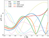 |
Fig. 1. Elements of the SDO/AIA response matrix 𝒬(T) as calculated with Eq. (17) for EBTEL covariance coefficients. Highlighted are the response functions corresponding to the 193 Å and 211 Å channels (green and blue), their cross-channel response (orange), and the composite response (red). |
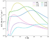 |
Fig. 2. Temperature response functions of the AIA channels. |
In order to infer the ϖ factor, one may stick to one of two strategies. One may first deduce the mean temperature μT (via, e.g., the filter-ratio technique) and then calculate ϖ by dividing any of the channels’ variances by the corresponding response. The main issue with this approach is connected with the nonmonotonicity of the 𝒬(T) functions, leading to ambiguities in temperature estimates. We, however, prefer another option. We aimed to eliminate the temperature dependence by constructing a composite channel with an almost flat response in the relevant temperature range so that it could be regarded as a direct proxy for ϖ. Unfortunately, there is no exact approach for mixing a perfect blend. However, we succeeded in finding a good combination for AIA. We propose to sum the 193 Å and 211 Å variances and subtract their cross-channel covariance. The given covariance response is plotted with a bold orange line in Fig. 1 (we note that it turns negative between 1.6 and 1.9 MK). The resulting composite response is plotted with a bold red line in the same figure (we emphasize that the line is flat between 1 and 1.8 MK). With the mean value of 7.3 in the given range, we could finally write down the explicit formula to infer ϖ based on AIA data:
![Mathematical equation: $$ \begin{aligned} \varpi = \frac{1}{7.3} \left( \frac{\sigma ^2[I_{193}]}{\mu ^2[I_{193}]} + \frac{\sigma ^2[I_{211}]}{\mu ^2[I_{211}]} - \frac{\mathrm{cov} [I_{193}, I_{211}]}{\mu [I_{193}] \mu [I_{211}]} \right). \end{aligned} $$](/articles/aa/full_html/2024/03/aa48425-23/aa48425-23-eq23.gif) (19)
(19)
Equation (19) loses its applicability outside the range of 1 to 1.8 MK. One can check the validity of the results via independent temperature estimation. For this, we propose a variation of the filter-ratio method, which aids in dealing with the nonmonotonicity of the channel responses. The main idea comes from the color management area. We note that if three channels are available (e.g., tristimulus values X, Y, and Z of the human eye sensitivity), then two linearly independent ratios may be derived: x = X/(X + Y + Z) and y = Y/(X + Y + Z). The xy plot for color perception is known as the chromaticity diagram (Smith & Guild 1931). We took the 193 Å channel response as X, the 211 Å channel as Y, and the composite response as the denominator. For a mono-temperature plasma, we obtained a parametric curve, plotted in Fig. 3, that is almost elliptical. A completely monotonic function starting with 1 MK and ending at 3.4 MK may be deduced to locate the point on the ellipse (e.g., a local azimuth θ relative to the ellipse center). We note that the temperature increases gradually from 1 MK to 2 MK for angles from 0 to 300 degrees, providing a decent resolution. The range of high angles is less valuable not only due to poorer resolution but also because of the subsequent discontinuity.
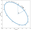 |
Fig. 3. SDO/AIA 193 and 211 Å channels’ xy “chromaticity” diagram. The ellipse-like figure is the mono-temperature locus, with temperatures shown in megakelvins. The azimuth θ can be used as a measure of the position on the ellipse and hence to estimate the temperature. |
At this point, we have defined all the key components of the developed method so that it can be applied to a set of AIA data. In the following section, we describe a small statistical trick that may ease the computation of intensity variances and increase the accuracy of the result.
3.2. Calculation of statistical moments
When calculating sample moments of the registered intensity, we needed to consider that the actual signal ξ is biased due to photon shot noise and dark noise (Makitalo & Foi 2013):
 (20)
(20)
where ψ ∼ 𝒫(I) stands for the number of absorbed photons, ϕ ∼ 𝒩(μD, σD) is the dark noise (in DNs), and η is the photons-to-counts conversion factor. The sample mean, variance, and cross-channel covariance of intensity are then
![Mathematical equation: $$ \begin{aligned}&\mu [I] = \frac{\mu [\xi ] - \mu _{\rm D}}{\eta }, \end{aligned} $$](/articles/aa/full_html/2024/03/aa48425-23/aa48425-23-eq25.gif) (21)
(21)
![Mathematical equation: $$ \begin{aligned}&\sigma ^2[I] = \frac{\sigma ^2[\xi ] - \sigma ^2_{\rm D}}{\eta ^2} - \mu [I], \end{aligned} $$](/articles/aa/full_html/2024/03/aa48425-23/aa48425-23-eq26.gif) (22)
(22)
![Mathematical equation: $$ \begin{aligned}&\mathrm{cov} [I_{193}, I_{211}] = \frac{\mathrm{cov[\xi _{193}, \xi _{211}] }}{\eta _{193} \eta _{211}}. \end{aligned} $$](/articles/aa/full_html/2024/03/aa48425-23/aa48425-23-eq27.gif) (23)
(23)
We note that the mean intensity value and the dark noise variance bias single channel variance. The cross-channel covariance is free from these issues because of the statistical independence of noise. Moreover, after substituting Eqs. (21) and (23) in Eq. (19), the η factors vanish. It then becomes very advantageous to compute auto-covariance with the lag of one frame instead of the actual variance,
![Mathematical equation: $$ \begin{aligned} \sigma ^2[I] \approx \frac{\mathrm{cov} [\xi (t_{i+1}), \xi (t_i)]}{\eta ^2}, \end{aligned} $$](/articles/aa/full_html/2024/03/aa48425-23/aa48425-23-eq28.gif) (24)
(24)
so that all the noise parameters also drop out from the equation. We note that the cost of this trick is a minor decrease in precision, which can be considered insignificant if considering the AIA cadence rate. With this remark, one may treat the intensities standing in Eq. (19) as count values registered by AIA sensors.
3.3. Image processing
We accessed the AIA data via the Joint Science Operations Center (JSOC) service. We downloaded the preprocessed level-1 full-resolution full-disk compressed .fits files for the 193 Å and 211 Å channels. The whole dataset contained 300 images in each channel. The only preprocessing we made was that we centered the images and compensated for the minor rolling and the Sun’s differential rotation. Since we did not want to interfere with the signal count statistics, we used nearest-neighbor interpolation instead of other options (e.g., bilinear or bicubic).
We then applied Welford’s online algorithm (Welford 1962) to perform a batch computation of pixel mean and variance for each channel and cross-channel covariances. Finally, we employed Eq. (19) to calculate ϖ and Fig. 3 to estimate μT at every pixel. The results and discussion of them are presented in the next section.
4. Results
4.1. Parameter ϖ
The map of the distribution of the measured ϖ values across the solar disk is depicted in Fig. 4. We note the pronounced uniformity of the distribution, with most pixel-wise ϖ values fitting within the same order of magnitude with the mean of ≈10−3. The disk edge is exceptionally sharp, with ittle to no apparent variability beyond it.
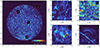 |
Fig. 4. Distribution of the variability factor ϖ across the solar disk (left panel) and close-up images of four noticeable pattern types (right panel). The identifiable patterns are: a) a diffuse patch, b) bright points, c) an AR-like region, and d) off-limb loops. |
Four different pattern types can be distinguished in the map, and the corresponding examples have been enlarged in the right panel of Fig. 4.
– Diffuse regions with no evident structure and low levels of ϖ (< 10−3) cover most of the surface (Fig. 4a). Even if these regions possess some inner structure, it is almost dissolved by the noise. The dark spots may be associated with either the increased frequency of heating (or, equivalently, continuous heating) or the lack of sensitivity due to the local decrease in temperature.
– Bright points represent compact sites of enhanced variability with ϖ > 10−2. Visually, the sources are distributed uniformly without a noticeable increase in number at certain latitudes. In the polar regions, helmet-like structures show the highest values (Fig. 4b), presumably due to low levels of base intensity. The inner structure is resolved poorly, mainly due to the small size (≲10 Mm).
– In resolved structures (loops, arcades, and small AR-like structures) the parameter ϖ takes intermediate values between the previous two types. As evident from the presented example (Fig. 4c), the apparent structure of these regions is highly stratified. While an individual loop can be traced well from one end to another, the neighboring loops significantly differ in brightness, signaling their uncorrelated dynamics. Resolution limits the ultimate loop thickness so that this behavior may remain at smaller scales.
– Off-limb structures (loops and streamers), despite low ϖ values, are visible to high altitudes, presumably due to the general drop in brightness (Fig. 4d). The longest loops can extend up to 100 Mm before fading to black completely. Interestingly, these structures seem thicker and less stratified than on-limb loops, so they are presumably heated in a more correlated manner.
The overall distribution histogram of ϖ calculated at every pixel on the disk is shown in Fig. 5. The distribution peaks at ϖ ≈ 3 × 10⁻⁴, corresponding to the dark spots of diffuse regions. Above it, the distribution fits well with a single power law ∼ϖ−2.6. The absence of peculiarities in this part of the plot implies the similarity of the registered dynamics.
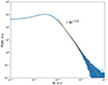 |
Fig. 5. Pixel-wise distribution histogram of the variability factor ϖ (blue) approximated with the power-law (orange). |
4.2. Temperature
The distribution of the mean temperature μT across the solar disk is presented in the left panel of Fig. 6. The right panel of the figure shows the close-ups of the same patches as in Fig. 4. The distribution is substantially uniform, with almost all the points lying inside the range from 1 MK to 2 MK. The narrowness of the range of observed plasma temperatures of quiescent coronal structures has been pointed out many times (for review, see Del Zanna & Mason 2018). There is no sign from the ϖ map of bright points being overheated relative to the background (compare Figs. 6a,b). Rare pulses occurring in these regions do not result in persistent heating. The hottest sites in the quiet corona are associated with either inner parts of AR-like structures (see Fig. 6c), similar to cores of regular ARs, or long off-limb loops (Fig. 6d). The latter presumably manifests the general scaling law T ∼ L1/3 (Martens 2010).
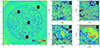 |
Fig. 6. Distribution of the mean temperature μT across the solar disk (left panel) and close-up images of the four noticeable pattern types (right panel). The four identifiable patterns are: a) a diffuse patch, b) bright points, c) an AR-like region, and d) off-limb loops. |
In Fig. 7, we plot the temperature diagram for the inner points of the disk. Most of the points fall inside the mono-temperature ellipse from Fig. 3. Moreover, most points are close to the ellipse, indicating that the line-of-sight temperature distribution is close to homogeneous. The estimated temperature range spans from 1.1 MK to 1.5 MK, with the mode of ≈1.25 MK in perfect agreement with the results of the spectroscopic diagnostics (Feldman et al. 1999; Del Zanna et al. 2008). The found temperatures fall into the applicability range of Eq. (19) and indicate the validity of the results obtained in Sect. 4.1.
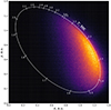 |
Fig. 7. Temperature diagram for the points inside the solar limb. The outer ellipse-like boundary is the mono-temperature locus; temperatures are shown in megakelvins. |
5. Discussion and conclusion
The presented results imply that the nanoflare heating (if it does take place) acts in a high-frequency regime. It follows that neighboring impulses highly overlap. Hence, the existing techniques based on detecting the separate events may not be as effective as previously thought (Krucker & Benz 1998; Aschwanden et al. 2000; Ulyanov et al. 2019b; Chitta et al. 2021). From this perspective, the observed impulsive dynamics should be regarded as a stochastic process rather than a group of separate events and treated accordingly.
We employed a novel model-based algorithm that we designed while keeping simplicity in mind so that our findings could be easily verified. We validated our approach by using it to estimate the temperature of the quiescent coronal structures and found good correspondence with independent studies. For example, Jess et al. (2019) employed Monte Carlo simulations to study nanoflare activity in active regions and found little excess variance in single-channel intensity fluctuations, which is on par with our results. Based on the inferences of a pretrained convolutional neural network (CNN), Upendran & Tripathi (2021) reported frequencies of two to three impulsive events per minute with a lifespan of 10–20 min, suggesting ϖ of 0.02–0.05, which is slightly higher than the values we obtained in our study.
We see several ways to improve the given technique. We are primarily concerned with two factors that could interfere with the results. First, the low-temperature background could add up to the average channel intensities. Secondly, the uncorrelatedness of the emitting volume at the line of sight could influence the variances. According to Eq. (6), both factors lead to the decrease of ϖ, and hence, the presented results should be regarded as lower limits. One way to deal with this issue is to increase the instrument’s spectral selectivity and resolution. For example, one may utilize the data of the Hi-C (High Resolution Coronal Imager; Kobayashi et al. 2014) rocket experiments or the novel Extreme Ultraviolet Imager (EUI; Rochus et al. 2020) instrument onboard the Solar Orbiter (Müller et al. 2020). An alternative is to introduce the corresponding modifications to the model. The recent 3D magnetohydrodynamic simulations by Knizhnik et al. (2020) showed that adjacent field lines exhibit collective cluster-like behavior during energization. Hence, we might expect our main findings to stay intact after the corrections.
The current study does not distinguish between various physical mechanisms that drive impulsive heating. It would be advantageous to compare our findings with the topological models of Parker (1972) and Priest et al. (2002) and recent studies, such as the stochastic reconnection model by Jafari et al. (2021). The high-resolution magnetic field data of the Polarimetric and Helioseismic Imager (PHI; Solanki et al. 2020) instrument may contribute greatly to this task.
While the anticipated dependency for shorter loops to have higher ϖ values is traced quite well, it is challenging to quantify. In order to measure the scale of the local coronal structure, one may employ magnetic field extrapolation techniques (for review, see Wiegelmann & Sakurai 2021) or train a CNN (e.g., ResNet, He et al. 2016) for this task.
The most significant advantage of the presented approach is that it allows for a seamless expansion. A more advanced model could replace EBTEL straightforwardly to account for the details of the chromospheric evaporation. Additional observational channels can also be introduced. With enough channels, it is possible to recover all the elements of the Q matrix and, hence, to verify the underlying model.
Acknowledgments
This research was funded by the Russian Science Foundation, project number 21-72-10157.
References
- Aschwanden, M. J., Nightingale, R. W., Tarbell, T. D., & Wolfson, C. J. 2000, ApJ, 535, 1027 [Google Scholar]
- Biermann, L. 1948, ZAp, 25, 161 [NASA ADS] [Google Scholar]
- Bogachev, S. A., Ulyanov, A. S., Kirichenko, A. S., Loboda, I. P., & Reva, A. A. 2020, Phys. Usp., 63, 783 [NASA ADS] [CrossRef] [Google Scholar]
- Brémaud, P. 2014, Fourier Analysis and Stochastic Processes, Universitext (Springer Cham) [CrossRef] [Google Scholar]
- Cargill, P. J. 2014, ApJ, 784, 49 [NASA ADS] [CrossRef] [Google Scholar]
- Chitta, L. P., Peter, H., & Young, P. R. 2021, A&A, 647, A159 [NASA ADS] [CrossRef] [EDP Sciences] [Google Scholar]
- Davila, J. M. 1987, ApJ, 317, 514 [NASA ADS] [CrossRef] [Google Scholar]
- Del Zanna, G., & Mason, H. E. 2018, Liv. Rev. Sol. Phys., 15, 5 [Google Scholar]
- Del Zanna, G., Rozum, I., & Badnell, N. R. 2008, A&A, 487, 1203 [NASA ADS] [CrossRef] [EDP Sciences] [Google Scholar]
- Del Zanna, G., Dere, K. P., Young, P. R., & Landi, E. 2021, ApJ, 909, 38 [NASA ADS] [CrossRef] [Google Scholar]
- Feldman, U., Doschek, G. A., Schühle, U., & Wilhelm, K. 1999, ApJ, 518, 500 [NASA ADS] [CrossRef] [Google Scholar]
- Gomez, D. O., Martens, P. C. H., & Golub, L. 1993, ApJ, 405, 773 [NASA ADS] [CrossRef] [Google Scholar]
- Hannah, I. G., Grefenstette, B. W., Smith, D. M., et al. 2016, ApJ, 820, L14 [NASA ADS] [CrossRef] [Google Scholar]
- He, K., Zhang, X., Ren, S., & Sun, J. 2016, in 2016 IEEE Conference on Computer Vision and Pattern Recognition (CVPR), 770 [Google Scholar]
- Ishikawa, S.-N., Glesener, L., Christe, S., et al. 2014, PASJ, 66, S15 [NASA ADS] [CrossRef] [Google Scholar]
- Jafari, A., Vishniac, E. T., & Xu, S. 2021, ApJ, 906, 109 [NASA ADS] [CrossRef] [Google Scholar]
- Jess, D. B., Dillon, C. J., Kirk, M. S., et al. 2019, ApJ, 871, 133 [Google Scholar]
- Klimchuk, J. A. 2015, Philos. Trans. R. Soc. London Ser. A, 373, 20140256 [NASA ADS] [Google Scholar]
- Klimchuk, J. A., Patsourakos, S., & Cargill, P. J. 2008, ApJ, 682, 1351 [Google Scholar]
- Knizhnik, K. J., Barnes, W. T., Reep, J. W., & Uritsky, V. M. 2020, ApJ, 899, 156 [NASA ADS] [CrossRef] [Google Scholar]
- Kobayashi, K., Cirtain, J., Winebarger, A. R., et al. 2014, Sol. Phs., 289, 4393 [CrossRef] [Google Scholar]
- Krucker, S., & Benz, A. O. 1998, ApJ, 501, L213 [Google Scholar]
- Lemen, J. R., Title, A. M., Akin, D. J., et al. 2011, Sol. Phys., 172 [Google Scholar]
- Levine, R. H. 1974, ApJ, 190, 457 [NASA ADS] [CrossRef] [Google Scholar]
- Makitalo, M., & Foi, A. 2013, IEEE Trans. Image Process., 22, 91 [CrossRef] [Google Scholar]
- Marsh, A. J., Smith, D. M., Glesener, L., et al. 2018, ApJ, 864, 5 [NASA ADS] [CrossRef] [Google Scholar]
- Martens, P. C. H. 2010, ApJ, 714, 1290 [NASA ADS] [CrossRef] [Google Scholar]
- Martens, P. C. H., Kankelborg, C. C., & Berger, T. E. 2000, ApJ, 537, 471 [NASA ADS] [CrossRef] [Google Scholar]
- Müller, D., St. Cyr, O. C., Zouganelis, I., et al. 2020, A&A, 642, A1 [Google Scholar]
- Parker, E. N. 1972, ApJ, 174, 499 [NASA ADS] [CrossRef] [Google Scholar]
- Parker, E. N. 1988, ApJ, 330, 474 [Google Scholar]
- Parnell, C. E., & Jupp, P. E. 2000, ApJ, 529, 554 [Google Scholar]
- Pesnell, W. D., Thompson, B. J., & Chamberlin, P. C. 2012, Sol. Phs., 275, 3 [CrossRef] [Google Scholar]
- Porter, J. G., Moore, R. L., Reichmann, E. J., Engvold, O., & Harvey, K. L. 1987, ApJ, 323, 380 [NASA ADS] [CrossRef] [Google Scholar]
- Priest, E. R., Heyvaerts, J. F., & Title, A. M. 2002, ApJ, 576, 533 [NASA ADS] [CrossRef] [Google Scholar]
- Reva, A., Ulyanov, A., Kirichenko, A., Bogachev, S., & Kuzin, S. 2018, Sol. Phys., 293, 140 [NASA ADS] [CrossRef] [Google Scholar]
- Rochus, P., Auchère, F., Berghmans, D., et al. 2020, A&A, 642, A8 [NASA ADS] [CrossRef] [EDP Sciences] [Google Scholar]
- Rosner, R., Tucker, W. H., & Vaiana, G. S. 1978, ApJ, 220, 643 [Google Scholar]
- Schwarzschild, M. 1948, ApJ, 107, 1 [Google Scholar]
- Smith, T., & Guild, J. 1931, Trans. Opt. Soc., 33, 73 [NASA ADS] [CrossRef] [Google Scholar]
- Solanki, S. K., del Toro Iniesta, J. C., Woch, J., et al. 2020, A&A, 642, A11 [NASA ADS] [CrossRef] [EDP Sciences] [Google Scholar]
- Sylwester, B., Sylwester, J., & Phillips, K. J. H. 2010, A&A, 514, A82 [NASA ADS] [CrossRef] [EDP Sciences] [Google Scholar]
- Ulyanov, A. S., Bogachev, S. A., Loboda, I. P., Reva, A. A., & Kirichenko, A. S. 2019a, Sol. Phys., 294, 128 [Google Scholar]
- Ulyanov, A. S., Bogachev, S. A., Reva, A. A., Kirichenko, A. S., & Loboda, I. P. 2019b, Astron. Lett., 45, 248 [CrossRef] [Google Scholar]
- Upendran, V., & Tripathi, D. 2021, ApJ, 916, 59 [NASA ADS] [CrossRef] [Google Scholar]
- Warren, H. P., Winebarger, A. R., & Brooks, D. H. 2012, ApJ, 759, 141 [NASA ADS] [CrossRef] [Google Scholar]
- Welford, B. P. 1962, Technometrics, 4, 419 [CrossRef] [Google Scholar]
- Wiegelmann, T., & Sakurai, T. 2021, Liv. Rev. Sol. Phys., 18, 1 [NASA ADS] [CrossRef] [Google Scholar]
- Withbroe, G. L., & Noyes, R. W. 1977, ARA&A, 15, 363 [Google Scholar]
- Wolter, K. M. 2007, Introduction to Variance Estimation, Springer Series in Statistics (New York, NY: Springer) [Google Scholar]
- Young, P. R., Viall, N. M., Kirk, M. S., Mason, E. I., & Chitta, L. P. 2021, Sol. Phs., 296, 181 [CrossRef] [Google Scholar]
- Zavershinskii, D. I., Bogachev, S. A., Belov, S. A., & Ledentsov, L. S. 2022, Astron. Lett., 48, 550 [NASA ADS] [CrossRef] [Google Scholar]
Appendix A: Covariance matrix calculation
A common solution of a system of linear ordinary differential equations is
 (A.1)
(A.1)
where we used the notation of matrix exponential, which can then be expanded, for example, via Sylvester’s formula:
 (A.2)
(A.2)
where α1, α2 are eigenvalues of A (which are generally complex) and 𝒜1, 𝒜2 are its Frobenius covariants:
 (A.3)
(A.3)
We can then compute the covariance matrix KXX ≡ cov[X, X] by multiplying Eq. A.1 by itself and then averaging over the ensemble of random heating functions:
![Mathematical equation: $$ \begin{aligned} \boldsymbol{K_{XX}}(t) = \omega ^2 \int \int \limits _0^t e^{\omega (\theta - t) \boldsymbol{A}}\mathrm{cov} [\boldsymbol{H}(\theta ), \boldsymbol{H}(\theta ^{\prime })] e^{\omega (\theta ^{\prime } - t) \boldsymbol{A}^\mathrm{T}}d\theta d\theta ^{\prime }. \end{aligned} $$](/articles/aa/full_html/2024/03/aa48425-23/aa48425-23-eq32.gif) (A.4)
(A.4)
As can be seen, the covariance of X should be the same for the classes of H with similar correlation functions. The standard approach assumes a delta correlation of H. However, we considered a broader class of exponentially correlated functions:
![Mathematical equation: $$ \begin{aligned} \mathrm{cov} [\boldsymbol{H}(\theta ), \boldsymbol{H}(\theta ^{\prime })] = \boldsymbol{K_{HH}} e^{-\lambda |\theta - \theta ^{\prime }|}, \end{aligned} $$](/articles/aa/full_html/2024/03/aa48425-23/aa48425-23-eq33.gif) (A.5)
(A.5)
where KHH is the covariance matrix of H. Substituting Eqs. A.2 and A.5 with Eq. A.4 and taking the limit t → +∞, one would obtain
 (A.6)
(A.6)
where
 (A.7)
(A.7)
We assumed the relaxation of the system to be slower than the characteristic heating rate so that λ ≫ ω, and hence,
 (A.8)
(A.8)
We also note that for the EBTEL equations, the calculation of KXX can be considerably simplified since KHH has only one non-zero component, and hence the variance of H (as well as ω/λ factor) may be brought forward
 (A.9)
(A.9)
where:
 (A.10)
In case of the EBTEL model, matrix Q has the following components:
 (A.11)
All Figures
|
Fig. 1. Elements of the SDO/AIA response matrix 𝒬(T) as calculated with Eq. (17) for EBTEL covariance coefficients. Highlighted are the response functions corresponding to the 193 Å and 211 Å channels (green and blue), their cross-channel response (orange), and the composite response (red). |
| In the text | |
|
Fig. 2. Temperature response functions of the AIA channels. |
| In the text | |
|
Fig. 3. SDO/AIA 193 and 211 Å channels’ xy “chromaticity” diagram. The ellipse-like figure is the mono-temperature locus, with temperatures shown in megakelvins. The azimuth θ can be used as a measure of the position on the ellipse and hence to estimate the temperature. |
| In the text | |
|
Fig. 4. Distribution of the variability factor ϖ across the solar disk (left panel) and close-up images of four noticeable pattern types (right panel). The identifiable patterns are: a) a diffuse patch, b) bright points, c) an AR-like region, and d) off-limb loops. |
| In the text | |
|
Fig. 5. Pixel-wise distribution histogram of the variability factor ϖ (blue) approximated with the power-law (orange). |
| In the text | |
|
Fig. 6. Distribution of the mean temperature μT across the solar disk (left panel) and close-up images of the four noticeable pattern types (right panel). The four identifiable patterns are: a) a diffuse patch, b) bright points, c) an AR-like region, and d) off-limb loops. |
| In the text | |
|
Fig. 7. Temperature diagram for the points inside the solar limb. The outer ellipse-like boundary is the mono-temperature locus; temperatures are shown in megakelvins. |
| In the text | |
Current usage metrics show cumulative count of Article Views (full-text article views including HTML views, PDF and ePub downloads, according to the available data) and Abstracts Views on Vision4Press platform.
Data correspond to usage on the plateform after 2015. The current usage metrics is available 48-96 hours after online publication and is updated daily on week days.
Initial download of the metrics may take a while.