| Issue |
A&A
Volume 690, October 2024
|
|
|---|---|---|
| Article Number | A23 | |
| Number of page(s) | 22 | |
| Section | Astrophysical processes | |
| DOI | https://doi.org/10.1051/0004-6361/202348268 | |
| Published online | 27 September 2024 | |
Dust evolution during a protostellar collapse: Influence on the coupling between the neutral gas and magnetic field
Université Paris-Saclay, Université Paris Cité, CEA, CNRS, AIM, 91191 Gif-sur-Yvette, France
Received:
13
October
2023
Accepted:
29
May
2024
Context. The extent of the coupling between the magnetic field and the gas during the collapsing phase of star-forming cores is strongly affected by the dust size distribution, which is expected to evolve by means of coagulation, fragmentation, and other collision outcomes.
Aims. We aim to investigate the influence of key parameters on the evolution of the dust distribution, as well as on the magnetic resistivities during protostellar collapse.
Methods. We performed a set of collapsing single-zone simulations with shark. The code computes the evolution of the dust distribution, accounting for different grain growth and destruction processes, with the grain collisions being driven by brownian motion, turbulence, and ambipolar drift. It also computes the charges carried by each grain species and the ion and electron densities, as well as the magnetic resistivities.
Results. We find that the dust distribution significantly evolves during the protostellar collapse, shaping the magnetic resistivities. The peak size of the distribution, population of small grains, and, consequently, the magnetic resistivities are controlled by both coagulation and fragmentation rates. Under standard assumptions, the small grains coagulate very early as they collide by ambipolar drift, yielding magnetic resistivities that are many orders of magnitude apart from the non-evolving dust case. In particular, the ambipolar resistivity, ηAD, is very high prior to nH = 1010 cm−3. As a consequence, magnetic braking is expected to be ineffective. In this case, large size protoplanetary discs should result, which is inconsistent with recent observations. To alleviate this tension, we identified mechanisms that are capable of reducing the ambipolar resistivity during the ensuing protostellar collapse. Among them, electrostatic repulsion and grain-grain erosion feature as the most promising approaches.
Conclusions. The evolution of the magnetic resistivities during the protostellar collapse and consequently the shape of the magnetic field in the early life of the protoplanetary disc strongly depends on the possibility to repopulate the small grains or to prevent their early coagulation. Therefore, it is crucial to better constrain the collision outcomes and the dust grain’s elastic properties, especially the grain’s surface energy based on both theoretical and experimental approaches.
Key words: hydrodynamics / magnetohydrodynamics (MHD) / turbulence / planets and satellites: formation / protoplanetary disks
© The Authors 2024
 Open Access article, published by EDP Sciences, under the terms of the Creative Commons Attribution License (https://creativecommons.org/licenses/by/4.0), which permits unrestricted use, distribution, and reproduction in any medium, provided the original work is properly cited.
This article is published in open access under the Subscribe to Open model. Subscribe to A&A to support open access publication.
1. Introduction
Interstellar dust plays a significant role in many astrophysical environments, in particular, in the context of star formation. Although it represents (on average) only 1% of the diffuse interstellar medium (ISM) mass, the wide spectrum of dust grain sizes affects the optical properties of the medium and, consequently, the heating and cooling processes at work (McKee & Ostriker 2007). In addition, dust grains are at the heart of many molecule formation processes (including H2Gould & Salpeter 1963). They are also the fundamental bricks of planets, which are believed to form rapidly in less than 1 Myr (Testi et al. 2014). The pathway to planetesimals and thereafter planets remains poorly understood. Getting a better description of the dust evolution during the protostellar collapse would allow us to provide more realistic dust initial conditions in protoplanetary discs. Finally, dust grains affect the ionisation degree of the medium and can become the main charge carriers during the protostellar collapse as they allow for electron and ion recombination and electron capture at their surface (Marchand et al. 2016). As such, they control the degree of coupling between the gas and the magnetic field (Nakano et al. 2002) via the ambipolar, Hall, and ohmic magnetic resistivities, and, consequently, the evolution of the angular momentum through magnetic braking (Mouschovias 1991). Indeed, dust plays a crucial role in shaping the magnetic field during the protostellar collapse and, thus, in influencing the structure of the resulting protoplanetary discs (Wurster et al. 2016, 2018; Hennebelle et al. 2020).
The dust size spectrum is observed or at least modelled as a power-law Mathis–Rumple–Nordsiek (MRN) distribution in the diffuse ISM (Mathis et al. 1977). It was noticed that modifying the population of very small grains in the protostellar collapse simulations radically affects the magnetic resistivities and, consequently, the formation of protoplanetary discs (Zhao et al. 2016; Marchand et al. 2016). In addition, the dust size distribution is expected to evolve as dust grains undergo coagulation and fragmentation processes (Dominik & Tielens 1997; Ormel et al. 2009). Following such an evolution of the dust distribution is very challenging, but it is essential to correctly describe the non-ideal MHD effects since the coupling between the grains, the gas, and the magnetic field depends directly on the total dust cross section. Indeed, Guillet et al. (2020), Silsbee et al. (2020) and Lebreuilly et al. (2023) showed that a coagulating dust distribution would affect the resistivities during the protostellar collapse. So far, only a handful of studies have accounted for dust coagulation in 2D (Vorobyov & Elbakyan 2019; Tu et al. 2022) or 3D (Tsukamoto et al. 2021, 2023; Bate 2022). Recently, Marchand et al. (2023) performed the first 3D simulations of the protostellar collapse and the early evolution of the protoplanetary disc, while including and self-consistently computing the magnetic field from the magnetic resistivities. The dust coagulation (fragmentation was not included) was modelled at low computational cost with a turbulent kernel (as described in Marchand et al. 2021), exerting an indirect feedback on the gas through the magnetic field, which allows us to better describe the effect of dust growth on non-ideal MHD effects. Similarly, Tsukamoto et al. (2023) used a dust single-size approximation and describe the co-evolution of dust grains and protoplanetary discs. Fragmentation has been introduced by Lebreuilly et al. (2023) and Kawasaki et al. (2022), and some parameters (turbulent intensity and velocity threshold for fragmentation) was investigated in more detail in Kawasaki & Machida (2023). They show that the interplay between coagulation and fragmentation plays a critical role in regard to the evolution of the magnetic resistivities. Indeed, those studies showed that fragmentation could potentially repopulate the small grains at intermediate and high densities, consequently allowing the Ohm and Hall resistivities to rise. The ambipolar resistivity, ηAD, was reduced to some extent prior to nH < 1010 cm−3 and enhanced thereafter. Besides, every study accounting for dust evolution produces magnetic resistivities, which remain remarkably away from the ones obtained with a non-evolving MRN distribution. This is even more striking when including ambipolar diffusion as a source of grain-grain collision, which is very efficient at depleting the smallest grains. For instance, as a consequence of small grain depletion by coagulation, the ambipolar resistivity, ηAD, exhibits very high values at low and intermediate densities. This would have a profound impact on the properties of the resulting protoplanetary discs. Given that recent observational surveys, including CALYPSO (Maury et al. 2019), have shown that large discs (> 60 AU) are rare, serious doubts are cast on the likeliness of such high ambipolar resistivity values.
To shed light on the impact of dust evolution on the magnetic resistivities during the protostellar collapse, we conducted a thorough investigation of the influence of key parameters and physical effects through single-zone collapse numerical simulations. In particular, we investigated the role of dust grain properties (grain surface energy, intrinsic density, monomer size), collision outcomes (fragments distribution, maximum fragment size, grain-grain erosion, sticking efficiency, electrostatic repulsion), and the collapse properties (dust-to-gas ratio, turbulence intensity, ambipolar drift intensity, initial magnetic field strength, and ionisation rate induced by cosmic rays). However, we focus only on the most influential of the aforementioned parameters and strive to identify mechanisms that would allow us to mitigate the sharp rise in ambipolar resistivity, ηAD.
In Sects. 2 and 3, we present the dust model and the numerical methods. Then, in Sects. 4 and 5, we share some of our results, which are discussed in Sect. 6. Finally, Sect. 7 provides concluding remarks and additional material can be found in the appendix.
2. Dust model
This numerical work is carried out with the shark code. More details regarding the methods employed and the structure of the code can be found in the associated paper (Lebreuilly et al. 2023).
2.1. Sources of dust relative velocities
Here, we present the different sources of relative velocities that drive dust evolution. In the rest of the paper, the subscripts i and j will refer to the two colliding grains.
2.1.1. Brownian motion
Dust grains are prone to Brownian motion, which is a thermal process that induces relative velocities as per:
where T is the gas temperature and kB the Boltzmann constant. This induced velocity is the highest for collisions including one grain much smaller than the other (or both small grains). Indeed in either case, the reduced mass in the square root is proportional to the mass of the smallest grain 
2.1.2. Ambipolar diffusion
Ambipolar diffusion emerges as a consequence of different coupling between the magnetic field and dust grains, the said coupling depending on their size. This coupling is embodied by the gyromagnetic frequency  . qi is the total charge carried by the grain,
  its mass, si its size and ρgrain is the grain bulk intrinsic density, taken to be equal to 2.3 g cm−3. B is the magnetic field intensity. Following the approach proposed by Guillet et al. (2020), the induced relative velocity between two grains is a function of their respective Hall factor, given by

where ts, i is the stopping time, representing the coupling of a grain to the gas (Epstein 1924):
where ρ and  are respectively the mass density of the gas and the sound speed. The number of charges carried by a grain increases slower with respect to grain size than the grain mass does. Therefore, larger grains are associated with lower gyromagnetic frequencies, namely, they are poorly coupled to the magnetic field. Besides, they are weakly coupled to the gas as well, as suggested by the size dependency of the stopping time. Nonetheless, the stopping time and the gyromagnetic timescale both rise with respect to the grain size, but the latter does so more rapidly. This leads in fine to lower Hall factors for larger grains.
As in Spitzer (1941), we define the ambipolar diffusion velocity as:
where c is the speed of light, ηAD is the ambipolar resistivity (in unit s). The curl of the magnetic field is approximated as  , where λJ is the Jeans length. Following Guillet et al. (2007, 2020), we have:
where δAD is the amibipolar drift intensity, taken equal to unity if not specified otherwise. We note that the larger the ambipolar resistivity, ηAD, the stronger the ambipolar drift velocity. Finally, the ambipolar drift velocity between two dust grains is given by:
Ambipolar drift allows for the largest grains to collect the smallest ones. Therefore, ambipolar diffusion is a process very effective at removing the smallest grains, but not at increasing significantly the maximum size of the distribution (Lebreuilly et al. 2023). Importantly, we stress that the ambipolar resistivity, ηAD, and the ambipolar drift intensity, δAD, are two different quantities, which should not be confused henceforth.
2.1.3. Turbulence
The vast spectrum of vorticies and eddies induced in a turbulent cascade can generate differential velocities between dust grains (Voelk et al. 1980). Indeed, a grain of given size couples with a variety of eddies and acquires a kick in the velocity space as a consequence. The analytical model used in this work is the one derived by Ormel & Cuzzi (2007). We follow the approach of Guillet et al. (2020) and assume the injection timescale of the turbulence to be the free-fall timescale

where ρ is the gas density and 𝒢 the universal gravitational constant. The dissipation timescale tη of the turbulence is then computed via the injection timescale and the Reynolds number (Ormel et al. 2009)

where
The Stokes number of a grain is defined as Sti = ts, i/tff, where the stopping time ts, i of the largest of the two grains determines the three coupling regimes defined in the framework of Ormel et al. (2009). The differential turbulent induced velocity writes:
where  and
and  , with xj, i being the ratio between Stj and Sti. The parameter θ is the turbulence intensity. The usual value taken in the literature in the context of a gravitational collapse is
  (Guillet et al. 2020).
When the stopping time of the largest grain is comprised between the dissipation timescale and the injection timescale (i.e. turnover time of the largest eddies), the contribution from class II eddies acts as a random kick in the grain motion, allowing for grains of similar size to efficiently collide (see Ormel & Cuzzi 2007, for a detailed definition of the class I, II and III eddies). This is the intermediate regime, which is the dominant regime in the context of the protostellar collapse (Marchand et al. 2021).
We note that the turbulent source of relative velocities is commonly found to be the most efficient at growing large grains and significantly increasing the maximum size of the dust distribution (Silsbee et al. 2020; Guillet et al. 2020; Lebreuilly et al. 2023).
2.2. Dust evolution
The different sources of relative velocity presented here lead to grain collisions that may result in various outcomes. In this work, we only account for grain coagulation (perfect and imperfect sticking) and fragmentation, and we also investigate the influence of grain-grain erosion with a simplistic approach. Many other mechanisms have been identified with laboratory experiments, such as gas-grain erosion, abrasion, compaction and bouncing, mass transfer, and rotational disruption (see Wurm & Teiser 2021, for more details). The grains are considered perfectly spherical, with a fixed and unique intrinsic density.
2.2.1. Coagulation
The equation of mass conservation for the grains is expressed as:
![$$ \begin{aligned} \frac{\partial \rho _{k} }{\partial t} +\nabla \cdot \left[ \rho _{k} \boldsymbol{v_k} \right] = S_{k,\mathrm{growth}}, \ \forall k \in \left[1,\mathcal{N} \right], \end{aligned} $$](/articles/aa/full_html/2024/10/aa48268-23/aa48268-23-eq19.gif)
The subscript k designates one specific grain among 𝒩 species. Here, the term species relates to a grain of given size. The source term Sk, growth accounts for coagulation and fragmentation events and is computed according to the Smoluchowski equation (Smoluchowski 1916):
where K is the coagulation kernel that embodies the microphysics of the collision. The first term highlights the increase in mass density of the grain k of mass mk ≡ mi + mj as a result of the sticking between two smaller grains i and j. The second term (a sink term) describes the reduction in mass density of the grain k for any sticking/coagulation it may undergo with an arbitrary grain i. ni is the number density of grains of mass mi such as ρi ≡ mi ni.
The coagulation kernel is expressed as
where Δvi, j is the differential velocity between grains i and j, of size si and sj, defined as the quadratic sum of the sources of differential velocity detailed in Sect. 2.1. The  pre-factor comes from considering that grains relative velocities along the three x, y, and z axis are Gaussian variables of variance Δvi, j2/3 (Guillet et al. 2020; Marchand et al. 2021). Here,
  is the kinetic energy of the colliding grains. μi, j ≡ mimj/(mi+mj) is the reduced mass of the two grains. Also, ECoulomb = qiqj/4πϵvacuum(si+sj) is the Coulomb electrostatic energy and ϵvacuum the vacuum dielectric permittivity. The first term in the Kernel accounts for the cross section modification induced by the electrostatic interaction between the two colliding grains (Akimkin et al. 2023). It is included only in the simulations for which electrostatic repulsion is explicitly investigated.
2.2.2. Fragmentation and elastic properties
To establish a fragmentation condition, we follow Ormel et al. (2009), whose work involves dust grains in quiescent environments, that is to say: porous aggregates colliding at subsonic velocities and made up of elementary, unbreakable pieces called monomers. Experimentally Blum & Wurm (2000) observed that complete fragmentation of the two colliding grains takes place as soon as the kinetic energy of the collision exceeds five times the total breaking energy, Ebr, tot = NtotEbr, of the grains (defined in Dominik & Tielens 1997):
where  is the total number of electrostatic bonds between monomers. Ebr is the energy required to break a single electrostatic bound and depends on the elastic properties of the grains, including the surface energy density γgrain and the reduced elastic modulus ε*. The latter is a function of the Poisson’s ratio and Young’s modulus, as detailed in Dominik & Tielens (1997). The mass of a monomer is related to the average monomer size as per
  where ρgrain is the bulk intrinsic density of the grains. We use Abr = 2.8 × 10³, which is experimentally measured in Blum & Wurm (2000). Here, smono is the monomer size, taken to be equal to 100 nm. We note that although Ebr diminishes when reducing the monomer size, the total breaking energy actually increases due to the increasing number of bonds Ntot. Consequently, reducing the monomer size leads to a higher fragmentation energy threshold.
3. Numerical methods
The numerical structure of the code used to treat the dust evolution has been thoroughly detailed in Lebreuilly et al. (2023). Here, we only shed light on the specific features relevant to our analysis. The version used here is the python sharkpy version. It accounts for dust evolution through coagulation and fragmentation processes, and computes the grain charge, ion, and electron number density as well as the magnetic conductivities and resistivities of the mixture. Within the scope of this work, the simulations were performed on a single cell, where physical properties can evolve with time, but with no spatial extension.
3.1. Dust
3.1.1. Coagulation and fragmentation
Unless otherwise specified, the total dust-to-gas ratio is taken to be ϵ0 = 0.01, and is spread over 𝒩 grain sizes (i.e. bins or species) on a logarithmic grid that ranges between smin and smax. The number of dust bins 𝒩 used in regard to the dust growth algorithm is inferred from the logarithmic increment, and the limits of the grid. The logarithmic increment writes:  . If the grid limits are to be modified, the logarithmic increment (i.e. the number of dust bins per decade) is held constant and we adjust the total number of dust bins accordingly, with the reference value (smin = 5×10⁻⁷ cm,smax = 1 cm) ⇒ 𝒩 = 300 extracted from a convergence test. The initial dust distribution is considered to be a power-law as:
  for the number density, or equivalently:
  in terms of mass dust-to-gas ratio, with
  and λ = −3.5.
For each collision between grains i and j, we define a fragmentation coefficient ffrag, i, j that is computed according to the fragmentation condition presented in Sect. 2.2.2 (and explained below). A fraction (1 − ffrag, i, j) (mi + mj) of the total mass involved in the collision is coagulated to form a larger grain. The rest of the mass, ffrag, i, j (mi + mj) = mfrag, is shattered and redistributed as fragments among all the bins in the range [mmin,0.1 mfrag], with mmin being the mass associated with the dust bin of size smin. The shattered mass mfrag is redistributed as a number density power-law:  , where ψ = −3.5.
We set ffrag = 1 when the fragmentation condition in Sect. 2.2.2 is met (corresponding to a complete fragmentation) and ffrag = 0 when  (corresponding to sheer coagulation). In between those limits, the fragmentation coefficient varies linearly with respect to the kinetic energy of the collision.
3.1.2. Grain-grain erosion
For some simulations, we constrain the fragmentation coefficient to be finite (0 < ffrag, min = fero) when the fragmentation criterion is not met, in such a way as to include a soft grain-grain erosion (Blum 2018).
Grain-grain erosion involves grains of very different sizes. Recently, Schrapler et al. (2018) conducted laboratory experiments to constrain the velocity threshold (for the onset of grain-grain erosion) and the corresponding efficiency by colliding micrometer projectiles onto a cm size target. They measured mass losses from the larger grain equal to a few times the mass of the smaller one in some cases. They observed the velocity threshold decreasing and the erosion efficiency rising when increasing the size difference between the projectile and the target. We assume their results can be translated to different grain size regimes (e.g. nanometer and micrometer grains at low density during the collapse). We implemented in our code the erosion velocity threshold (Fig. 8 in their paper) as a function of the grain size ratio sratio = starget/sprojectile (where starget is the size of the larger grain and sprojectile that of the smaller)
![$$ \begin{aligned} \mathrm{log} \left(V_{\rm erosion} \right) = \frac{\mathrm{log}\left(3 \right)}{\mathrm{log}\left(0.2\right)} \mathrm{log}\left(s_{\rm ratio}\right) + \mathrm{log} \left(45 \right) - 2 \frac{\mathrm{log}\left(3\right)}{\mathrm{log}\left(0.2\right)} \ \left[\mathrm{m\,s}^{-1}\right], \end{aligned} $$](/articles/aa/full_html/2024/10/aa48268-23/aa48268-23-eq34.gif)
and the erosion efficiency (Fig. 7 in their paper):
where Δv is the relative collision velocity between both grains.
3.1.3. Electrostatic repulsion
Since grains are negatively charged on average, they experience electrostatic repulsion as they encounter, which modifies their effective collisional cross-section (see Eq. (13)). In addition, we allow for coagulation only if the kinetic energy of the colliding grains is higher than the Coulomb electrostatic energy (Ekinetic > ECoulomb). This translates into a velocity threshold that needs to be exceeded for the colliding grains to stick together:
This velocity condition is included only in the simulations for which electrostatic repulsion is explicitly investigated.
3.1.4. Charging and resistivities
We used the scheme presented in Marchand et al. (2021) to compute the charge of each grain species and the number density of ions and electrons. It relies on different parameters such as the average ion (HCO+) mass μions = 25, the size of ice coats sice = 8 nm, the sticking efficiency coefficient of electrons onto grains se = 0.5 and the cosmic-ray ionisation rate ζ = 5 × 10⁻¹⁷s−1.
The conductivities (parallel, perpendicular and Hall) are inferred via the Hall factor (Eq. (2)) and the individual conductivities of the different species:
In turn, the ohmic, ambipolar and Hall resistivities are computed as
To better understand the behavior of the resistivities, in Appendix , we include the conductivity profiles, with an emphasis on the distinct influence of the different species, namely, the electrons, the ions and the grains.
3.2. Setups
3.2.1. Magnetic field
We use an analytical expression that allows for the magnetic field to increase with the density as per Li et al. (2011) and Marchand et al. (2016):
where B0 = 30 μG is the magnetic field intensity at nH = 104 cm−3. We define the ambipolar diffusion timescale as:

where c is the speed of light and r the distance from the center of the collapsing cloud.
3.2.2. Collapse setup
This single zone setup reproduces the gravitational collapse of a protostellar cloud up to the formation of the first Larson core.
The temperature is computed according to a barotropic equation used in Machida et al. (2006) and Marchand et al. (2016, 2021):
where the initial cloud temperature T0 = 10 K is a typical value measured in dense prestellar cores. Also, nH, ad is the threshold density that marks the transition between the isothermal and the adiabatic regime, usually nH, ad ≃ 1011 cm−3. We consider a perfect gas with equation of state:

where Pg is the gas pressure, ρ is the mass density of the gas, μg = 2.3 is the mean molecular weight, and mH is the mass of a hydrogen atom. The sound speed is given by  , where the effective adiabatic index is taken to be that of a monoatomic gas
  since the temperature of H2 molecules is not high enough to excite vibrational and rotational energy states in this cold environment. Figure 1 gives the gas density evolution with time during the protostellar collapse. The data is extracted from the central cell of a shark 1D collapse simulation without rotation or magnetic support. The collapse is initiated and halted exactly as in Lebreuilly et al. (2023), that is, to say with an initial density of ρ = 9.2 × 10⁻¹⁸ g cm−3(nH = 2.4×106 cm−3) and a final density of ρ = 10−10 g cm−3(nH = 2.6×1013 cm−3), which corresponds to a solar mass cloud associated with a gravitational to thermal energy ratio α = 0.25.
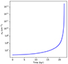 |
Fig. 1. Gas numerical density evolution with time throughout the gravitational collapse. |
In Appendix B.2, we offer a comparison between a non-evolving MRN dust distribution, a growing distribution and a growing plus fragmenting distribution at different instants of the collapse. We recovered the results of Lebreuilly et al. (2023) and Kawasaki et al. (2022).
3.2.3. Parameters investigated
Table 1 displays the parameters explored and their corresponding values. We highlight in bold in the first column the reference values used when a given parameter is not being varied (note: we used two reference values for the grain surface energy γgrain). From those reference values, we vary the parameters independently, one at a time.
-
γgrain is the surface energy of the grains, which controls the breaking energy. Given the uncertainties around the elastic properties and tensile strength of the grains, and given that there is a temperature dependency of the surface energy of the grains, we vary the latter between two extreme values measured in Musiolik & Wurm (2019): γgrain = 2.9 erg cm−2 and γgrain = 190 erg cm−2. Using the elastic modulus for icy-grains to be ε* = 3.7 × 10¹⁰, the two extreme values for the surface energy correspond respectively to the case of minimum breaking energy (Ebr, min = 1.27 × 10⁻¹⁰ erg) and maximum breaking energy (Ebr, max = 4.11 × 10⁻⁷ erg) we could encounter.
-
Erosion is a boolean that activates or deactivates the grain-grain erosion process.
-
Repulsion is a boolean that activates or deactivates the grain-grain electrostatic repulsion process.
-
δAD is the ambipolar drift intensity, taking values between 0.1 and 10. Those limit values are expected in collapsing environments, as suggested by Fig. D.1.
-
B0 is the initial magnetic field strength corresponding to a gas density of nH = 104 cm−3 in the scaling approximation of Eq. (21). It takes values between 10−5 G and 5 × 10⁻⁵ G, which are common values measured in dense cores, see for example Troland & Crutcher (2008).
-
ζ is the ionisation rate induced by cosmic rays. (see Sect. 3.1.4). It takes values between 5 × 10⁻¹⁸ s−1 and 5 × 10⁻¹⁶ s−1, which are typical values measured in Padovani et al. (2022). Constraining this parameter is a daunting task due to the uncertainties in the chemical networks used and to observation difficulties.
-
ϵstick is a grain sticking coefficient which affects the sticking probability between two colliding grains, but not that of fragmentation. It takes values between 0.1 and 1. Since this parameter is poorly constrained and dependent on the grain surface energy and grain coats nature, we explored a wide range of values.
Range of values taken by the explored parameters.
4. Results
We first explored the impact of the surface energy of the grains. Then, we found that the degree of influence of the other parameters depends strongly on the fragmentation rate, that is on the grain surface energy. Consequently, we do not make any assumption regarding the composition of the grains but rather choose to investigate the influence of the other parameters for two different extreme values of the grain surface energy, corresponding to resistant grains (γgrain = 190 erg cm−2) on one hand, and fragile ones (γgrain = 10 erg cm−2) on the other hand. We investigate the influence of the ambipolar drift intensity and its combined effect with electrostatic repulsion and grain-grain erosion for a grain surface energy of γgrain = 190 erg cm−2. The analysis of the grain-grain sticking efficiency ϵstick is given in the appendix (Fig. F.1), performed with γgrain = 190 erg cm−2. The initial magnetic field strength B0 and the cosmic-ray ionisation rate ζ are mentioned and commented on in Sect. 5 (γgrain = 190 erg cm−2 if not specified otherwise).
4.1. Impact of the surface energy of the grains γgrain
The surface energy is the most influential grain property in regard to fragmentation, since the breaking energy scales as  (see Eq. (15)). As a reminder, the correct value is still subject to debate in the literature.
Figure 2 depicts the evolution of the dust mass distribution (first row) and dust number distribution (second row) at different densities during the protostellar collapse, for different values of the grain surface energy. The third row displays the Ohm, ambipolar, Hall resistivities, ion and electron numerical densities evolution with gas density. Likewise for the last row, but with the conductivities and the peak size of the dust distribution. The magnetic resistivities associated with a fixed MRN dust distribution are displayed as a reference in black dashed lines. The impact of the grain surface energy is striking. Indeed, for values of γgrain = 10 erg cm−2 and below, fragmentation comes in very early as a replenishment of the population of small grains. It is observed already at nH = 108 cm−3. Conversely for larger values, fragmentation only appears at densities higher than nH = 1010 cm−3, and is even completely absent for γgrain = 190 erg cm−2. The peak size of the distribution is lower when decreasing the surface energy: indeed at the end of the collapse, the peak size is of the order of 0.1 mm for the lowest value of γgrain while it can reach a value of 1 mm in the case of the largest grain surface energies. In summary, a lower grain surface energy thus entails more fragile grains, which leads to a more rapid and efficient replenishment of the population of small grains along with a reduced peak size of the dust distribution at the end of the collapse.
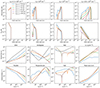 |
Fig. 2. Dust distributions at different stages during the collapse. First row: Mass dust-to-gas ratio. Second row: Number dust-to-gas ratio. Third row: Resistivities profile and ion and electron numerical densities (Hall resistivity: dotted line for the negative values and solid line for the positive ones). Dashed black lines: Reference resistivities obtained with a fixed MRN dust distribution. Fourth row: Parallel, perpendicular, and Hall conductivities, and the evolution of the peak size of the dust distribution. Comparison between different values of the grain surface energy expressed in cgs units (erg cm−2). |
Such variations in the population of small grains at low densities lead to significant variations in the resistivities. Indeed, for γgrain = 2.9 erg cm−2, the immediate replenishment of small grains at all densities gives rise to a subsequent much higher Ohm resistivity throughout the collapse, even at low densities. For γgrain = 10 erg cm−2, fragmentation occurs early but slightly later than γgrain = 2.9 erg cm−2, and consequently the effects on the Ohm resistivity only emerge later on, as we need the density to sufficiently increase in order for the excess of small grains to collect the electrons. Indeed, a higher number of small grains implies a larger overall cross-section for electron capture by dust grains. This capture reduces the electron density and thus enhances the ohmic resistivity. The ambipolar resistivity ηAD is sensitive to the population of small grains as well. In reducing the value of the surface energy of the grains, the small grain re-population results in a higher dust conductivity contribution (which, along with the ions, is the prevailing contribution here; see Appendix ) and thus to a lower ambipolar resistivity ηAD at low and intermediate densities. At high densities, the ambipolar resistivity is controlled by the ion density only, and the ambipolar resistivity appears as larger since the excess of small grains reduces the ion density by means of ion-electron recombination at their surface. Finally, the Hall resistivity is very sensitive to the population of small grains and reducing the surface energy induces a re-population of the latter, leading to a transition between negative and positive values that is shifted to higher densities. This transition is even completely suppressed for the lowest value of γgrain, which displays a Hall resistivity profile quite similar to that of a fixed MRN distribution (represented as a black dashed line). Indeed, the Hall resistivity is very sensitive to the relative number of electrons and ions. A change in the number of small grains induces a change in the relative number densities of electrons and ions which can easily lead to a change of sign of the Hall resistivity. The more numerous the small grains, the later the transition (change of sign) occurs (see Appendix for a better description of the Hall conductivity sensitivity to the dust distribution). Depending on the sign of the Hall resistivity, the Hall effect can either promote or reduce the rotation of the collapsing core.
Since the ambipolar resistivity ηAD dominates over the Ohm resistivity, we can conclude that more fragile grains (i.e. enhanced fragmentation) leads to a less efficient magnetic diffusion at low and intermediate densities (nH ≲ 1010 cm−3), but more efficient at high density.
4.2. Exploration for γgrain = 190 erg cm−2
We go on to consider the case of resilient grains for which fragmentation is substantially curtailed.
4.2.1. Impact of grain-grain erosion
Here, we explore the impact of grain-grain erosion that can serve as an alternative to fragmentation to repopulate the small grains. We note on Fig. 3 the replenishment of the population of very small grains induced by erosion and the limited impact it has on the magnetic resistivities at low density. However, the said impact gets stronger with density as the largest grains grow, allowing for larger grain size ratios and collisional velocities. We recall that according to Eq. (17), the erosion efficiency augments for increasing grain size ratio and grain collisional velocity. In effect, while the model without erosion exhibits a clearly diminishing dust number distribution as the collapse proceeds, the model with erosion maintains a constant population of small grains, with a value hovering around  . The rise in erosion efficiency is conspicuous when looking at the mass distribution at the end of the collapse, where not only the tail of the distribution is affected but the distribution as a whole. Consequently, the eroding collisions between the small grains and the largest ones tend to lower the dust peak size at high density. To recapitulate, under standard assumptions (fiducial values for the other parameters) the ambipolar resistivity, ηAD, is only slightly reduced prior to nH = 1011 cm−3 because the collisions involve grains with three orders of magnitude difference in size at most (collisions between nanometer and micrometer grains). At high density however, the dust distribution spans a much larger range of sizes and thus erosion is much more efficient (the said efficiency increases with the size difference between colliding grains). Consequently, the ambipolar and ohmic resistivities sharply rise, reaching values similar to the MRN case. The Hall resistivity is significantly affected for all densities nH > 108 cm−3. Again, in this case, the excess of small grains enabled by erosion processes shifts the change of sign to higher densities. We stress that at high densities, grain-grain erosion significantly reduces the departure from the MRN reference in terms of magnetic resistivities.
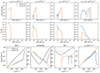 |
Fig. 3. Same as Fig. 2, but investigating the influence of grain-grain erosion with γgrain = 190 erg cm−2. |
4.2.2. Impact of the ambipolar drift intensity, δAD
We now turn our attention to the impact of the ambipolar drift intensity δAD, which controls the amplitude of the collisional velocities induced by ambipolar diffusion (ambipolar drift velocity), as suggested in Eq. (5). In particular, we focus on its combined effect with grain-grain erosion and electrostatic repulsion. Figure 4 depicts the ambipolar resistivity ηAD evolution during the protostellar collapse with and without electrostatic repulsion between dust grains, with and without grain-grain erosion for different values of the ambipolar drift intensity. The second row conveys the same information but with a lower grain-grain sticking efficiency (ϵstrick = 0.5). The same plot but for the ohmic resistivity can be found in the appendix (see Fig. E.1).
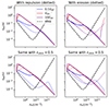 |
Fig. 4. Ambipolar resistivity ηAD evolution during the protostellar collapse for different values of the ambipolar drift intensity or equivalently different ambipolar drift velocities: δAD = 0.1 (0.1VAD), δAD = 1 (VAD), and δAD = 10 (10VAD). Grain-grain electrostatic repulsion (first column) and erosion (second column) are also included (dotted lines). Second row: Same details, but with a sticking efficiency of 0.5. |
First of all, by looking at the solid lines of the top left panel, we clearly see that reducing the ambipolar drift between grains alone leads to lower collisional velocities and thus to a much slower coagulation of the small grains. Their number drops less dramatically and consequently ambipolar resistivity ηAD is reduced at low density. Then, we turn on electrostatic repulsion (dotted lines) and remark that it has no impact whatsoever on the dust evolution when considering the reference values for the parameters (i.e. δAD = 1) because while Brownian motion is incapable of generating sufficiently large collisional velocities, the electrostatic barrier is easily overcome by the ambipolar diffusion drift (which allows for small grains to be collected by larger grains). However in reducing the ambipolar drift intensity to δAD = 0.1, we allowed the grains to experience collisional velocities lower than the Coulomb velocity threshold, thus inhibiting grain coagulation at low and intermediate densities, as suggested by Fig. 4. Indeed, with this scenario, the difference between the resulting ambipolar resistivity ηAD and that associated with an MRN dust distribution is of one order of magnitude at most. Then, as the collapse proceeds and the density increases, the peak size of the dust distribution increases as well and ultimately the largest grains manage to collect the smallest ones via ambipolar drift even for low values of δAD, and the three dotted lines end up overlapping. This is due to the fact that the larger the difference in size (or equivalently in Hall factor), the higher the relative collisional velocity induced by ambipolar diffusion (ambipolar drift velocity), see Eq. (6).
In addition, we see on the top right panel that for δAD = 1, erosion is influential at high density only, as previously highlighted in Sect. 4.2.1. However, for δAD = 10, while electrostatic repulsion has no impact, grain-grain erosion is rendered very efficient even at low densities due to the large collisional velocities at play. Thus, the significant subsequent replenishment of small grains produces an ambipolar resistivity ηAD remarkably lower, close to the MRN case. Those two effects (electrostatic repulsion and erosion) can operate jointly at the same time but respectively allow us to reduce the ambipolar resistivity in different circumstances and environments.
Finally, for δAD = 1, a look at the second row shows that a lower sticking efficiency slows down the coagulation of small grains (see Fig. F.1 for a more detailed impact of the sticking efficiency). For δAD = 0.1, the combined effect of electrostatic repulsion and a lower sticking efficiency yields an even more evident reduction of the ambipolar resistivity. For δAD = 10, the very strong erosion is almost not affected by the reduced sticking efficiency. However, note that the replenishment of small grains induced by erosion at high densities in the case of δAD = 0.1 and δAD = 1 is suppressed since half of the collisions lead to bouncing instead of erosion.
In summary, on one hand, if the ambipolar drift is sufficiently weak, erosion has no influence but electrostatic repulsion inhibits small grains depletion as they repel each other instead of sticking. On the other hand, if the ambipolar drift is sufficiently strong, the Coulomb barrier is easily overcome but grain-grain erosion is efficient enough to repopulate the small grains and consequently lower the ambipolar resistivity ηAD. We note that Appendix D explores the expected values of δAD within a collapsing core.
5. Dust growth: Potential consequences for the magnetic flux
Assuming standard conditions (reference values for the parameters), but varying the initial magnetic field B0 (see Eq. (21)) and the ambipolar drift intensity δAD, we can focus on the evolution of the ambipolar resistivity, ηAD, and on the ambipolar diffusion timescale, tAD, (see Eq. (22)) during the collapse.
The results of Sect. 4 highlight a tendency for the magnetic resistivities to be significantly different from those one gets with a fixed MRN distribution. In particular, the ambipolar resistivity ηAD exhibits high values at low and intermediate densities due to small grain depletion enabled by ambipolar drift. Indeed, since the small grains contribute directly to the perpendicular conductivity at low density (see Appendix ), their removal leads to a sharp increase in the ambipolar resistivity. At high density however, the perpendicular conductivity is controlled by the ionic contribution. In the absence of small grains, ions, and electrons do not efficiently recombine and thus the ion density remains high. Therefore at high density, the ambipolar resistivity, ηAD, is much lower with respect to the MRN case. The Ohm resistivity remains lower throughout the collapse, and monotonically increases. Unlike the fixed MRN case, the Hall resistivity systematically switches sign at some point, the corresponding density at which this transition occurs being highly sensitive to the dust distribution.
5.1. Small grain depletion: Grains cease to be the main charge carriers
Placing ourselves under standard assumptions, Fig. 5 depicts the evolution of the ambipolar resistivity ηAD during the collapse in the case of resilient grains (γgrain = 190 erg cm−2) for different values of the initial magnetic field strength B0. The dashed lines represent the fixed MRN reference case. The resistivity is normalized with B02 in such a way as to remove the direct dependency in B2 and isolate and focus on the influence of the ambipolar diffusion on the resistivity. We wish to see to what extent the ηAD ∝ B2 trend is relevant in the case of an evolving dust distribution. On Fig. 5, we can see that for different values of the initial magnetic field strength, the normalized ambipolar resistivities  rapidly converge and overlap once the small grains have been removed, which hints at a B2 dependency given by the analytical approximation,
  (Duffin & Pudritz 2008), with γin as the drag coefficient between ions and neutrals, then ρi and ρn as the mass density of the ion and neutral fluids. This analytical expression, which is derived in considering only electrons and ions as charged species, holds true here because the small grains (which contributes to the ambipolar resistivity) are rapidly depleted by the ambipolar diffusion drift. Indeed, this is depicted by the sharp rise in the ambipolar resistivity, ηAD, at the beginning of the collapse, the removal of small grains being even faster for a higher initial magnetic field strength (green curve). Considering a balance between ionisation by cosmic-rays and ion/electron recombination, we have
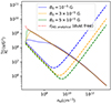 |
Fig. 5. Ambipolar resistivity, ηAD, (normalized with the squared initial magnetic field strength) evolution with gas density throughout the protostellar collapse, for different values of the initial magnetic field strength. Solid lines: growing dust distribution (γgrain = 190 erg cm−2). Dashed lines: non evolving MRN dust distribution. Dotted red line is the analytical dust-free solution. |
for the numerical ion density when dust is negligible. Here, ζ is the ionisation rate induced by cosmic rays and  is the ion/electron recombination rate determined in Marchand et al. (2021). To confirm this B2 trend, we use directly the expression of the ambipolar resistivity ηAD given by Eq. (20) to derive a complete expression. The parallel conductivity is dominated by the electron contribution. In absence of dust, the perpendicular one is dominated by the ion and the Hall conductivity is close to zero. Given that σelectron ≫ σion, perp and Γion ≫ 1 we find that once the small grains have been removed, the ambipolar resistivity scales as

where we considered  to switch from B to nH, where σion is the individual ion conductivity. e is the electric charge, c the speed of light in vacuum, and μion = 25 (for HCO+ ions considered) and τion is the ion reduced temperature. vion is the thermal speed of the ions, and kB is the Boltzmann constant. We recover the analytical form found in Duffin & Pudritz (2008). We overlay this analytical solution (dotted red curve) and see that it matches very well the numerical results, except of course at the first instants of the collapse, prior to small grain depletion.
5.2. A hint at a magnetic flux regulation
Figure 6 pictures the evolution of the ambipolar diffusion timescale for different values of the ambipolar drift intensity δAD (see Eq. (5)) in the case of resilient grains (solid lines) and fragile grains (dotted lines, γgrain = 10 erg cm−2). We can see on Fig. 6 that given the very high ambipolar resistivity ηAD at low density caused by the very swift depletion of small grains, the ambipolar diffusion timescale drops rapidly to a value very close to the free-fall timescale. As a consequence, the magnetic field should diffuse more efficiently. If tAD > tff, the magnetic field strength should increase however less rapidly than the square root scaling of Eq. (21). If tAD = tff, it should dwell on its initial value since the increase in magnetic field by contraction of the flux tubes would be perfectly balanced by diffusion, or even decrease if tAD < tff. It is only later on when the resistivity has sufficiently dropped that the magnetic field recouples to the gas and should increase with respect to the density.
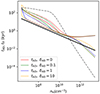 |
Fig. 6. Freefall timescale (in black) and ambipolar diffusion timescale as a function of gas density throughout the protostellar collapse for different values of the ambipolar drift intensity. The dashed grey line represents the fixed MRN case. The solid lines correspond to resistant grains (γgrain = 190 erg cm−2) whereas the dotted lines correspond to the fragile grains (γgrain = 10 erg cm−2). |
The ambipolar drift can be enhanced by either increasing the magnetic field strength or raising δAD. When fragmentation is inefficient (γgrain = 190 erg cm−2), we can see on Fig. 6 that in increasing the ambipolar drift intensity, the small grains are more swiftly depleted and thus the ambipolar diffusion timescale drops more rapidly. In addition, Fig. 5 shows that a higher magnetic field allows for the ambipolar resistivity, ηAD, to rise more rapidly, which entails an ambipolar diffusion timescale dropping faster. Therefore we can identify here a mechanism of magnetic flux regulation. The higher the magnetic field, the stronger the ambipolar drift, the faster the small grains are removed and thus the faster the magnetic field diffuses. However when considering an efficient fragmentation (γgrain = 10 erg cm−2, dotted lines), the trend is the same except for high values of the ambipolar diffusion intensity. Indeed, in going from δAD = 1 to δAD = 10, it takes more time for the ambipolar diffusion timescale to drop, thus suppressing the magnetic flux regulation mechanism. This is due to the fact that for such fragile grains and high δAD, the ambipolar diffusion drift between dust grains induces destructive collisions leading to a replenishment of the small grains instead of a depletion of the latter.
5.3. Saturation of the magnetic field
Finally, Fig. 7 displays the evolution of the ambipolar diffusion timescale for different values of the initial magnetic field strength and ionisation rate induced by cosmic rays. The black line represents the free-fall timescale. The ambipolar diffusion timescale is computed via Eq. (22) where each gas density is associated with a radius, r, assuming a singular isothermal sphere (see Shu 1977)

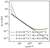 |
Fig. 7. Freefall timescale (in black) and ambipolar diffusion timescale as a function of gas density throughout the protostellar collapse for different values of the ionisation rate induced by cosmic rays. The initial magnetic field chosen corresponds to the critical value (minimum value) above which the small grain depletion leads to an ambipolar diffusion timescale lower than the freefall timescale. |
We can see that for a given value of the ionisation rate ζ, there exists a critical value of the initial magnetic field for which the ambipolar diffusion timescale will inexorably drop to equate the freefall timescale. When it does so, the magnetic field diffuses in such a way as to remain constant. The larger the cosmic-rays ionisation rate, the better is the coupling between the plasma and the magnetic field (i.e. the lower the ambipolar resistivity, ηAD). Consequently a higher initial magnetic field B0 is needed to produce an ambipolar drift strong enough to remove the small grains and, thus, to allow the magnetic field to diffuse significantly (i.e. to ensure that tAD = tff).
In such circumstances, we can define a saturation magnetic field that cannot be exceeded. We start from tAD = tff and assume that the ambipolar resistivity ηAD is controlled by the ion contribution, just as we did before. Using the analytical expression for ηAD which is plotted on Fig. 5, the previously defined expression for the ion reduced temperature, the free-fall timescale defined in Eqs. (7) and (25), we get:
Whatever the initial magnetic field strength B0, the small grains will be removed, preventing the magnetic field strength from exceeding the value deduced from Eq. (28). We stress that this expression is valid as long as the dust contribution is absent, that is to say prior to a potential significant replenishment of the small grains by fragmentation, and in the first instants of the collapse once they have been removed. We note, however, that at high densities in protoplanetary discs, the fragmentation barrier could be potentially reached after a few orbital periods, allowing for the small grain populations to be replenished and consequently allowing the gas and the magnetic field to decouple once more – in regions where the temperature is below the sublimation temperature of the dust (T ∼ 1500 K) and where the ionisation induced by the protostar is negligible. Also, with rotation and magnetic pressure, the free-fall timescale should be longer and therefore diffusion of the magnetic flux would be even easier.
6. Discussion
6.1. Considering whether there is a small grain depletion catastrophe
In light of the soaring of the ambipolar resistivity, ηAD, at low density resulting from dust coagulation, we may wonder whether small grain depletion has catastrophic consequences on protoplanetary disc formation.
6.1.1. Tensions with observed discs size
Indeed, this paradigm is in tension with recent astronomical observations of protoplanetary discs, which appear to be rather small in size. Several surveys have been carried out, including CALYPSO (Maury et al. 2019) for which less than 25% of the Class 0 protostellar discs exhibit a radius > 60 AU. Large discs seem to be rare and the observations favor the magnetized models of rotating protostellar collapse. This idea is supported by pure hydrodynamical numerical simulations which yield a too high occurence of large discs (Masson et al. 2016). Even though turbulence effects can reduce the disc sizes without the need of a magnetic field (see Bate 2018), the inclusion of a magnetic field produces much smaller discs (Hennebelle et al. 2020; Lee et al. 2021), more in agreement with observations. In their simulations of protoplanetary discs within massive star forming clumps, Lebreuilly et al. (2021) report a dominant population of small discs in both the ideal and non-ideal MHD (using an ambipolar resistivity obtained for a fixed MRN dust distribution) cases. For instance with ideal MHD, more than half of their disc population exhibit radii < 50 AU at the very early stages. When considering a higher ambipolar resistivity (via a truncated MRN dust distribution), Marchand et al. (2020) produce large discs while Zhao et al. (2016) suggest the possibility to form moderate protoplanetary disc sizes (a few tens of AU) when removing the smallest grains of the MRN dust distribution (grain sizes below 10 nm). Although different codes have been used, this discrepancy between both studies is most likely due to the 30° angle set between the rotation axis of the core and the magnetic field in the first study as opposed to the perfect alignment in the second. Indeed, a misalignment between both axes tends to reduce magnetic breaking efficiency although not significantly in non-ideal MHD (Masson et al. 2016). Non-ideal effects are needed to prevent the magnetic braking catastrophe, but should be sufficiently weak in such a way as to produce disc sizes and outflows consistent with observations.
6.1.2. Ways to preserve the small grain population
To alleviate the tension with observations, we identified several mechanisms preventing the small grains from being too severely depleted, thereby allowing us to reduce the ambipolar resistivity ηAD prior to nH = 1010 cm−3.
Considering fragile grains: Fig. 2 shows that values of  yield a much lower ambipolar resistivity ηAD at intermediate densities as a consequence of the small grain replenishment induced by grain fragmentation. Since the elastic properties of the grains are quite uncertain, this scenario cannot be discarded.
Low grain-grain sticking efficiency: Likewise the surface energy of the grains, this parameter remains poorly constrained. As depicted on Fig. F.1, allowing for one collision event out of ten to result in grain sticking allows us to recover an MRN-like ambipolar resistivity ηAD profile. In this case, the depletion of small grains is substantially curtailed.
Strong or weak ambipolar drift: The ambipolar drift intensity δAD appears as a prefactor in the ambipolar drift (Eq. (5)) and embodies our ignorance of the phenomena. For instance, the current (the curl of the magnetic field) is approximated here using the Jeans length  . This approximation is arguably simplistic and ignores directional effects inherent to a multi-dimensional problem. Indeed, it is well known that ambipolar diffusion is anisotropic and do not affect currents parallel to the magnetic field, as suggested by the cross product in Eq. (4). Ignoring here electrostatic repulsion and grain-grain erosion, Fig. 4 exhibits a lower ambipolar resistivity ηAD when reducing δAD by one order of magnitude.
Erosion: Even with resilient grains, erosion is capable of efficiently repopulating the small grains at low density provided that the ambipolar drift is strong enough (δAD = 10 on Fig. 4). Note that other destructive processes such as abrasion, gas-grain erosion, rotational disruption or grain sputtering could potentially enhance small grain replenishment as well.
Electrostatic repulsion: With the reference value δAD = 1, the ambipolar drift generates grain collisional velocities larger than the velocity threshold imposed by the Coulomb barrier (see Eq. (18)). However, this is no longer the case when reducing the ambipolar drift intensity to δAD = 0.1. As a consequence, small grain depletion is further hindered and the combined effect of a lower ambipolar drift intensity and grain electrostatic repulsion leads to a significant reduction of the ambipolar resistivity ηAD (see Fig. 4). Similarly, keeping δAD = 1, we notice that reducing the initial magnetic field generates a weaker ambipolar drift. Our simulations show that for an initial magnetic field strength (at nH = 104 cm−3) of B0 ≤ B0, min = 10 μG (for ζ = 5 × 10⁻¹⁷ s−1 and δAD = 1, that is for an initial current strength of  ), electrostatic repulsion effectively mitigates small grain coagulation and leads to a substantially lower ambipolar resistivity ηAD. Equation (21) is then a good approximation and the magnetic field can amplify in the early phase of the collapse. The value B0, min below which electrostatic repulsion comes into play is somehow almost insensitive to the cosmic ionisation rate. We measured values between 9.5 μG and 13.4 μG for ζ in the range [5×10−18,5×10−16] s−1. However, it should be kept in mind that although the population of small grains is preserved and the ambipolar resistivity is significantly reduced, a lower initial magnetic field (i.e. a higher mass-to-flux ratio) entails a weaker magnetic braking.
Relying on electrostatic repulsion or erosion, we see from Fig. 4 that in either scenario, the difference between the computed ambipolar resistivity value and that associated with an MRN dust distribution is of one order of magnitude at most (the ratio ranges between 2 at low density and 10 shortly before nH = 1010 cm−3). Relying on the analytical formulae for the radius of the early protoplanetary disc derived in Hennebelle et al. (2016) ( , and see Lee et al. (2024) for an extension to misalignment between magnetic field and rotation axis), we find that the corresponding difference in disc size would be of a factor of
  in the worst case, in contrast to a factor of
  without repulsion or erosion. Comparing now the MRN case with the coagulation-repulsion case with a lower sticking efficiency (ϵstick = 0.5), we find a factor of
  . In terms of actual disc size values, we gather in Table 2 the comparison between the different scenarios and readily see that we obtain reasonable disc radii with either repulsion or erosion. The initial vertical magnetic field is assumed to be Bz = 30 μG, and the star/disc system mass to be M = 0.1 M⊙ (consistent with a class 0 disc produced by the collapse of a one solar mass dense core). The ambipolar resistivity values ηAD are taken at the point of maximum departure from the MRN value, namely, slightly before nH = 1010 cm−3.
Disc radius rAD for different scenarios.
For intermediate values of ambipolar drift intensity, δAD, neither electrostatic repulsion nor grain-grain erosion can significantly reduce the ambipolar resistivity. In such circumstances, we need to rely on other levers such as fragile grains or low sticking efficiency. However, the appendix offers a map of the ambipolar drift intensity δAD in a collapsing core extracted from a 3D RAMSES (Teyssier 2002; Fromang et al. 2006) simulation performed by Lebreuilly et al. (2020); namely, model mmMRNmhd at t = 80 Kyr (Fig. D.1). It is inferred by measuring the Lorentz force (∇×B) × B and comparing it with the approximation  . As clearly seen, the intermediate value δAD = 1 is scarce, while both larger and lower values are ubiquitous. In the most central region (very young, nascent protoplanetary disc and core), and at large scale in the pseudo-disc, the ambipolar drift intensity dwells around δAD = 10. Consequently, grain-grain erosion is expected to induce a significant replenishment of the population of small grains in those denser regions. In contrast, the ambipolar drift intensity is much weaker (δAD ∼ 0.1) in the rest of the domain, which hints at an inhibition of small grain coagulation via electrostatic repulsion in those diffuse regions. This reinforces the fundamental role that both mechanisms, electrostatic repulsion and grain-grain erosion, play in maintaining a reasonable ambipolar resistivity, ηAD, during the protostellar collapse.
6.2. Resilient grains or fragile grains: Uncertainties in the collision outcomes
Uncertainties remain in regard to the description of collision outcomes. We recall here that some of them have been ignored in this work (see Wurm & Teiser 2021; Blum 2018 for a detailed list). Bouncing for example, is expected to occur prior to fragmentation, and leads to compaction in place of grain sticking. The bouncing barrier has been widely described in the literature (Zsom et al. 2010). Erosion as a consequence of grain-gas drag could replenish the system with small grains but is expected to be relevant mainly in protoplanetary discs where dust grains can experience a strong gas head wind (Rozner et al. 2020). More relevant to our environment is grain-grain erosion (Gundlach & Blum 2015; Schrapler et al. 2018) whose influence has been investigated in this work. We based our model on the experimental results of Schrapler et al. (2018). In this regard, we found that grain-grain erosion is unconditionally very efficient at high density, where collisional velocities and size ratios are large, leading to noticeable variations in the Ohm and ambipolar resistivities. However, it is efficient at low density only for sufficiently strong ambipolar drifts. Therefore, given the essential role of this process, future laboratory experiments will have to reinforce our understanding of this collision outcome and to further constrain the velocity threshold and efficiency. Additionally, electrostatic and magnetic reactions resulting from the charges carried by the grains may affect dust growth. In UV-shielded regions (where the grain photo-ionisation is negligible), the electrons are abundant (ne > ndust, i.e. efficient gas ionisation), plasma charging dominates, and dust grains are expected to be negatively charged, on average (Draine & Sutin 1987), electrostatic forces thus being repulsive and detrimental to grain coagulation (Okuzumi 2009; Akimkin et al. 2020). When accounting for dust fragmentation and electrostatic repulsion, the population of sub-micron grains was found to be enhanced and the dust coagulation/fragmentation equilibrium to be severely affected (see Akimkin et al. (2023) who consider hot UV-shielded regions of protoplanetary discs where gas thermal ionisation is important, with T = 1000 K and ρ = 10−12 g cm−3). In the context of protostellar collapse, since the densities involved are very low, we believe that between two consecutive grain-grain collisions, the dust particles would have sufficient time to settle back to their average equilibrium negative charge value imposed by their interaction with electrons and ions. In this case, dust grains would feel repulsive electrostatic forces. As discussed previously, this can curtail to some extent the very efficient coagulation observed at the very beginning of the collapse.
Moreover, the conditions needed for sticking and fragmentation are diverse. Those relevant to a dense core environment are not well constrained in the literature either, and not well reproduced in laboratory experiments. That is why we explored a wide range of grain surface energies γgrain. For instance, collision outcomes for icy-grains have turned out to be temperature dependent (Gärtner et al. 2017). Also, icy-grains have been believed to be stickier that bare-silicate grains (Gundlach et al. 2011; Drazkowska 2017), thus enhancing coagulation and being less prone to bouncing and compaction. Nevertheless, recent studies revealed that the grain surface energy γgrain (which controls both the sticking efficiency and the fragmentation threshold) of icy-grains could sharply decrease from T = 200 K to T = 175 K due to a change in the crystal structure (again within the frame of the laboratory experiments, where P = 1 bar and consequently the ice melting temperature being T = 273 K). Their measurements suggested a grain surface energy ranging between  at low temperature and γgrain = 190 erg cm−2 at higher temperature, which are the limit values we used in this work. For more details, refer to Musiolik & Wurm (2019). Note however that amorphous ice at low pressure and temperature could recover an efficient sticking under UV irradiation (Musiolik 2021). We explored the impact of the grain sticking efficiency in Fig. F.1 and found that values above 0.3 do not prevent the population of small grains from being depleted at low densities, thus allowing the ambipolar resistivity ηAD to dwell on very large values.
6.3. Uncertainties in the turbulence model
In this work, we rely on the model presented in Ormel et al. (2009) to compute the turbulent induced collisional velocities between dust grains. This model assumes a Kolmogorov cascade of the turbulence, which is not necessarily expected in core collapse environments where magnetic and gravitational effects are likely to affect the nature of this energy cascade. In their recent work, Gong et al. (2021) expanded this model for different energy cascades. Moreover, there is a necessity to go beyond the approximations inherent to this model and to account for the back reaction of the dust onto the gas, which is not negligible in regions of high dust-to-gas ratio and at small scales. This backreaction would affect the behavior of the turbulence and has been showed to alter the propagation of Alfven waves (Hennebelle & Lebreuilly 2023). Also, in order to better assess the turbulence induced collisional velocities, one needs to account for the magnetic field and the Lorentz force felt by the dust grains. Those refinements regarding the turbulence model would affect the growth of the peak size of the dust distribution and the replenishment of small grains via fragmentation of the largest ones.
In addition, turbulence can affect the local dust-to-gas ratio at small scales which is an essential ingredient in the context of dust growth. Indeed the turbulent coagulation timescale scales as the inverse of the dust-to-gas ratio squared. Turbulent motions are known to be capable of triggering hydrodynamics instabilities, allowing the dust-to-gas ratio to increase in certain regions (Kelvin–Helmholtz instability for instance, see Hendrix & Keppens 2014). Dust clumping by supersonic turbulence has been observed numerically in an environment reproducing molecular cloud physical conditions in Commerçon et al. (2023), and in Hopkins & Lee (2016) for supersonic MHD turbulence. With both an analytical and numerical approach, Hopkins & Squire (2018a) expanded their own work on the Resonant Drag Instability (RDI) by including the role of magnetic fields and charged dust. As the dust and the gas drift relative to each other (e.g. via gravity), instabilities develop for all modes wavelength, leading to strong fluctuations in the dynamics of both fluids. In addition to the purely hydrodynamical instabilities observed in their previous work (Hopkins & Squire 2018b; Squire & Hopkins 2018), they identified a whole set of new instabilities. More generally, hydrodynamical instabilities represent promising mechanisms to enable the formation of planetesimals.
7. Conclusion
In this work, we study how the evolution of the dust distribution could affect the degree of coupling between the gas and the magnetic field of a collapsing core, including both the coagulation and fragmentation of dust grains. We also investigated the effect of grain-grain erosion, but we neglected other collision outcomes such as compaction, bouncing, and rotational disruption. We used the shark code to self-consistently follow the evolution of the dust distribution and the subsequent impact on the magnetic resistivities. The code includes brownian motion, turbulence and ambipolar drift as grain-grain collision sources. We performed single zone simulations to save computational time and focus on the influence of fragmentation and various parameters. In summary, we found:
-
As in previous studies (Guillet et al. 2020; Kawasaki et al. 2022; Lebreuilly et al. 2023; Marchand et al. 2023), dust growth is found to be significant and the subsequent impact on the magnetic resistivities very important. Therefore, dust evolution cannot be disregarded in numerical simulations.
-
The degree of influence of the parameters depends on the fragmentation efficiency, which is primarily controlled by the grain surface energy. When considering a high value for this parameter (γgrain = 190 erg cm−2, i.e. resistant grains), fragmentation is substantially suppressed and the magnetic resistivities are only sensitive to the parameters which do not affect only (or not at all) the fragmentation processes; namely, the ambipolar drift intensity, the grain-grain erosion efficiency, electrostatic repulsion, and the cosmic-ray ionisation rate. However, when considering a low value for the grain surface energy (γgrain = 10 erg cm−2, fragile grains), fragmentation is severe and fragmentation-related parameters, such as the monomer size, the grain intrinsic density, and the power-law index of the fragment redistribution law become influential.
-
Grain fragmentation offers a way to replenish the population of small grains, which, in turn, significantly affects the resistivities. However, except for cases of very severe fragmentation, we find that the small grains are very rapidly removed due to ambipolar drift. As a consequence, the ohmic resistivity, ηO, remains negligible with respect to the ambipolar resistivity, ηAD, for the entirety of the collapse. In addition, the ambipolar resistivity is much higher at low densities and much lower at high densities than the value one gets in considering a fixed MRN dust distribution. Increasing the initial magnetic field strength leads to a more efficient depletion of small grains by ambipolar drift and a sharper rise in the ambipolar resistivity. The magnetic field then diffuses more rapidly, thus hinting at the regulation of the magnetic flux by ambipolar diffusion.
-
To alleviate the tension between the remarkably high ambipolar resistivities obtained in our simulations and the statistically low protoplanetary disc sizes observed, we identified a few mechanisms that allow for the ambipolar resistivity, ηAD, to be reduced and, thus, to supposedly enhance magnetic braking: low grain surface energy (i.e. fragile grains), high ionisation rate via cosmic rays and low grain-grain sticking efficiency. In addition, we show that for a sufficiently low ambipolar drift on one hand, grain-grain electrostatic repulsion efficiently inhibits small grain depletion, leading to a much lower ambipolar resistivity prior of nH = 1011 cm−3 (whereas the grain-grain erosion is negligible). On the other hand, in the case of a strong ambipolar drift, the Coulomb barrier for electrostatic repulsion is easily overcome, however, grain-grain erosion causes a significant replenishment of the small grains; consequently, there is a sharp reduction of the ambipolar resistivity as a result. Both effects are expected to maintain a reasonable ambipolar resistivity, ηAD, during the protostellar collapse.
-
We pointed out the uncertainties regarding the elastic properties of the grains and the fragmentation model. Given the dramatic influence fragmentation can have on the magnetic resistivities, it is fundamental to better constrain the grain surface energy and the various collision outcomes relevant to interstellar dust in the adequate range of grain sizes. In addition, the grain surface energy also controls the maximum size dust grains can reach by the end of the collapse. For γgrain = 10 erg cm−2, the grains grow up to 0.1 mm while for γgrain = 190 erg cm−2, we manage to form grains of a few mm.
As a last note, we recall that we used the square root approximation of Eq. (21) to compute the evolution of the magnetic field during the gravitational collapse as a function of the gas density only. However, the magnetic field affects the resistivities, which should (in turn) control the evolution of the latter through the induction equation and so forth. To rigorously describe the evolution of the magnetic field, multidimensional simulations, including dust growth along with a self-consistent computation of the magnetic field are needed.
Acknowledgments
We thank the referee who helped us greatly in improving the clarity and relevancy of this paper. We thank the consortium and ERC (European Research Council) synergy grant ECOGAL (grant 855130) for their financial support, and members for their contribution through insightful ideas and remarks.
References
- Akimkin, V. V., Ivlev, A. V., & Caselli, P. 2020, ApJ, 889, 64 [NASA ADS] [CrossRef] [Google Scholar]
- Akimkin, V., Ivlev, A. V., Caselli, P., Gong, M., & Silsbee, K. 2023, ApJ, 953, 72 [NASA ADS] [CrossRef] [Google Scholar]
- Bate, M. R. 2018, MNRAS, 475, 5618 [Google Scholar]
- Bate, M. R. 2022, MNRAS, 514, 2145 [CrossRef] [Google Scholar]
- Blum, J. 2018, Space Sci. Rev., 214, 52 [NASA ADS] [CrossRef] [Google Scholar]
- Blum, J., & Wurm, G. 2000, Icarus, 143, 138 [NASA ADS] [CrossRef] [Google Scholar]
- Commerçon, B., Lebreuilly, U., Price, D. J., et al. 2023, A&A, 671, A128 [NASA ADS] [CrossRef] [EDP Sciences] [Google Scholar]
- Dominik, C., & Tielens, A. G. G. M. 1997, ApJ, 480, 647 [Google Scholar]
- Draine, B. T., & Sutin, B. 1987, ApJ, 320, 803 [NASA ADS] [CrossRef] [Google Scholar]
- Drazkowska, J. 2017, European Planetary Science Congress, EPSC2017–815 [Google Scholar]
- Duffin, D. F., & Pudritz, R. E. 2008, MNRAS, 391, 1659 [NASA ADS] [CrossRef] [Google Scholar]
- Epstein, P. S. 1924, Phys. Rev., 23, 710 [Google Scholar]
- Fromang, S., Hennebelle, P., & Teyssier, R. 2006, A&A, 457, 371 [NASA ADS] [CrossRef] [EDP Sciences] [Google Scholar]
- Gärtner, S., Gundlach, B., Headen, T. F., et al. 2017, ApJ, 848, 96 [CrossRef] [Google Scholar]
- Gong, M., Ivlev, A. V., Akimkin, V., & Caselli, P. 2021, ApJ, 917, 82 [NASA ADS] [CrossRef] [Google Scholar]
- Gould, R. J., & Salpeter, E. E. 1963, ApJ, 138, 393 [NASA ADS] [CrossRef] [Google Scholar]
- Guillet, V., Pineau Des Forêts, G., & Jones, A. P. 2007, A&A, 476, 263 [NASA ADS] [CrossRef] [EDP Sciences] [Google Scholar]
- Guillet, V., Hennebelle, P., Pineau des Forêts, G., et al. 2020, A&A, 643, A17 [EDP Sciences] [Google Scholar]
- Gundlach, B., & Blum, J. 2015, ApJ, 798, 34 [Google Scholar]
- Gundlach, B., Kilias, S., Beitz, E., & Blum, J. 2011, Icarus, 214, 717 [Google Scholar]
- Hendrix, T., & Keppens, R. 2014, A&A, 562, A114 [NASA ADS] [CrossRef] [EDP Sciences] [Google Scholar]
- Hennebelle, P., & Lebreuilly, U. 2023, A&A, 674, A149 [NASA ADS] [CrossRef] [EDP Sciences] [Google Scholar]
- Hennebelle, P., Commerçon, B., Chabrier, G., & Marchand, P. 2016, ApJ, 830, L8 [Google Scholar]
- Hennebelle, P., Commerçon, B., Lee, Y.-N., & Chabrier, G. 2020, ApJ, 904, 194 [NASA ADS] [CrossRef] [Google Scholar]
- Hopkins, P. F., & Lee, H. 2016, MNRAS, 456, 4174 [Google Scholar]
- Hopkins, P. F., & Squire, J. 2018a, MNRAS, 479, 4681 [CrossRef] [Google Scholar]
- Hopkins, P. F., & Squire, J. 2018b, MNRAS, 480, 2813 [Google Scholar]
- Kawasaki, Y., & Machida, M. N. 2023, MNRAS, 522, 3679 [NASA ADS] [CrossRef] [Google Scholar]
- Kawasaki, Y., Koga, S., & Machida, M. N. 2022, MNRAS, 515, 2072 [NASA ADS] [CrossRef] [Google Scholar]
- Lebreuilly, U., Commerçon, B., & Laibe, G. 2020, A&A, 641, A112 [EDP Sciences] [Google Scholar]
- Lebreuilly, U., Hennebelle, P., Colman, T., et al. 2021, ApJ, 917, L10 [NASA ADS] [CrossRef] [Google Scholar]
- Lebreuilly, U., Vallucci-Goy, V., Guillet, V., Lombart, M., & Marchand, P. 2023, MNRAS, 518, 3326 [Google Scholar]
- Lee, Y.-N., Marchand, P., Liu, Y.-H., & Hennebelle, P. 2021, ApJ, 922, 36 [NASA ADS] [CrossRef] [Google Scholar]
- Lee, Y.-N., Ray, B., Marchand, P., & Hennebelle, P. 2024, ApJ, 961, L28 [NASA ADS] [CrossRef] [Google Scholar]
- Li, Z.-Y., Krasnopolsky, R., & Shang, H. 2011, ApJ, 738, 180 [Google Scholar]
- Machida, M. N., Inutsuka, S.-i., & Matsumoto, T. 2006, ApJ, 647, L151 [NASA ADS] [CrossRef] [Google Scholar]
- Marchand, P., Masson, J., Chabrier, G., et al. 2016, A&A, 592, A18 [NASA ADS] [CrossRef] [EDP Sciences] [Google Scholar]
- Marchand, P., Tomida, K., Tanaka, K. E. I., Commerçon, B., & Chabrier, G. 2020, ApJ, 900, 180 [CrossRef] [Google Scholar]
- Marchand, P., Guillet, V., Lebreuilly, U., & Mac Low, M. M. 2021, A&A, 649, A50 [NASA ADS] [CrossRef] [EDP Sciences] [Google Scholar]
- Marchand, P., Lebreuilly, U., Mac Low, M. M., & Guillet, V. 2023, A&A, 670, A61 [NASA ADS] [CrossRef] [EDP Sciences] [Google Scholar]
- Masson, J., Chabrier, G., Hennebelle, P., Vaytet, N., & Commerçon, B. 2016, A&A, 587, A32 [NASA ADS] [CrossRef] [EDP Sciences] [Google Scholar]
- Mathis, J. S., Rumpl, W., & Nordsieck, K. H. 1977, ApJ, 217, 425 [Google Scholar]
- Maury, A. J., André, P., Testi, L., et al. 2019, A&A, 621, A76 [NASA ADS] [CrossRef] [EDP Sciences] [Google Scholar]
- McKee, C. F., & Ostriker, E. C. 2007, ARA&A, 45, 565 [Google Scholar]
- Mouschovias, T. C. 1991, ApJ, 373, 169 [NASA ADS] [CrossRef] [Google Scholar]
- Musiolik, G. 2021, MNRAS, 506, 5153 [CrossRef] [Google Scholar]
- Musiolik, G., & Wurm, G. 2019, ApJ, 873, 58 [NASA ADS] [CrossRef] [Google Scholar]
- Nakano, T., Nishi, R., & Umebayashi, T. 2002, ApJ, 573, 199 [Google Scholar]
- Okuzumi, S. 2009, ApJ, 698, 1122 [Google Scholar]
- Ormel, C. W., & Cuzzi, J. N. 2007, A&A, 466, 413 [NASA ADS] [CrossRef] [EDP Sciences] [Google Scholar]
- Ormel, C. W., Paszun, D., Dominik, C., & Tielens, A. G. G. M. 2009, A&A, 502, 845 [NASA ADS] [CrossRef] [EDP Sciences] [Google Scholar]
- Padovani, M., Bialy, S., Galli, D., et al. 2022, A&A, 658, A189 [NASA ADS] [CrossRef] [EDP Sciences] [Google Scholar]
- Rozner, M., Grishin, E., & Perets, H. B. 2020, MNRAS, 496, 4827 [NASA ADS] [CrossRef] [Google Scholar]
- Schrapler, R., Blum, J., Krijt, S., & Raabe, J.-H. 2018, ApJ, 853, 74 [NASA ADS] [CrossRef] [Google Scholar]
- Shu, F. H. 1977, ApJ, 214, 488 [Google Scholar]
- Silsbee, K., Ivlev, A. V., Sipilä, O., Caselli, P., & Zhao, B. 2020, A&A, 641, A39 [NASA ADS] [CrossRef] [EDP Sciences] [Google Scholar]
- Smoluchowski, M. V. 1916, Z. Phys., 17, 557 [NASA ADS] [Google Scholar]
- Spitzer, L., Jr. 1941, ApJ, 93, 369 [NASA ADS] [CrossRef] [Google Scholar]
- Squire, J., & Hopkins, P. F. 2018, MNRAS, 477, 5011 [Google Scholar]
- Testi, L., Birnstiel, T., Ricci, L., et al. 2014, in Protostars and Planets VI, eds. H. Beuther, R. S. Klessen, C. P. Dullemond, & T. Henning (Tucson: University of Arizona Press), 339 [Google Scholar]
- Teyssier, R. 2002, A&A, 385, 337 [CrossRef] [EDP Sciences] [Google Scholar]
- Troland, T. H., & Crutcher, R. M. 2008, ApJ, 680, 457 [NASA ADS] [CrossRef] [Google Scholar]
- Tsukamoto, Y., Machida, M. N., & Inutsuka, S.-i. 2021, ApJ, 920, L35 [NASA ADS] [CrossRef] [Google Scholar]
- Tsukamoto, Y., Machida, M. N., & Inutsuka, S.-i. 2023, PASJ, 75, 835 [NASA ADS] [CrossRef] [Google Scholar]
- Tu, Y., Li, Z.-Y., & Lam, K. H. 2022, MNRAS, 515, 4780 [NASA ADS] [CrossRef] [Google Scholar]
- Voelk, H. J., Jones, F. C., Morfill, G. E., & Roeser, S. 1980, A&A, 85, 316 [Google Scholar]
- Vorobyov, E. I., & Elbakyan, V. G. 2019, A&A, 631, A1 [NASA ADS] [CrossRef] [EDP Sciences] [Google Scholar]
- Wurm, G., & Teiser, J. 2021, Nat. Rev. Phys., 3, 405 [CrossRef] [Google Scholar]
- Wurster, J., Price, D. J., & Bate, M. R. 2016, MNRAS, 457, 1037 [Google Scholar]
- Wurster, J., Bate, M. R., & Price, D. J. 2018, MNRAS, 475, 1859 [NASA ADS] [CrossRef] [Google Scholar]
- Zhao, B., Caselli, P., Li, Z.-Y., et al. 2016, MNRAS, 460, 2050 [Google Scholar]
- Zsom, A., Ormel, C., Blum, J., Guettler, C., & Dullemond, C. 2010, EGU Gen. Assembly Conf. Abstr., 2966 [Google Scholar]
Appendix A: Which species controls the conductivities during collapse
Figure A.1 explicitly shows that the individual electronic conductivity largely prevails over the others by a few orders of magnitude. Consequently, the total parallel conductivity is controlled by the electrons. In reducing the surface energy of the grains, γgrain, we allow for the small grains to be repopulated and to efficiently collect the electrons, resulting in a weaker overall parallel conductivity. Since the collision rate between small grains and electrons increases with density (regardless of dust coagulation), the impact on the electron conductivity and thus on the parallel conductivity only appears tardily in the collapse. Indeed, the dashed line diverges from the solid line at high densities only. The same reasoning is valid for the ions whose conductivity decreases as they recombine with electrons at the grains surface.
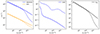 |
Fig. A.1. Individual conductivities profiles. The third panel displays the parallel conductivity. The solid lines correspond to the solid grain case (γgrain = 190 erg cm−2) and the dashed lines to the fragile grain case (γgrain = 10 erg cm−2). |
Regarding the individual perpendicular conductivities, the electronic contribution is negligible. Indeed, Fig. A.2 suggests that the total perpendicular conductivity is dominated by both the dust and the ions at low density. Eventually as the density goes up, the dust influence vanishes and the ions prevail. In enhancing fragmentation, the replenishment of small grains gives rise to a higher dust perpendicular conductivity (the large grains contribution is insignificant) which leads to a higher total perpendicular conductivity at low density (nH ≤ 109 cm−3). This effect is instantaneous since it does not involve any capture or interaction whatsoever. On the third panel, we can see that the dashed and solid lines overlap as soon as the dust ceases to be the dominant species, and the detachment between both curves at high densities is due to the ion density diminution (caused by electron/ion recombination) being significant at high densities only. We can derive an analytical formulae of a threshold value above which the ion density allows for the ion perpendicular conductivity to be larger than the dust perpendicular conductivity, namely, when σperp, ion > σperp, dust. When this condition is satisfied, the ambipolar resistivity ηAD becomes independent on the number of small grains, which explains why strong variations in the population of small grains sometimes do not reflect on the ambipolar resistivity (see for example Fig. 3 at nH = 108 cm−3). Using the expressions of Eq. (19), we get:
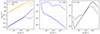 |
Fig. A.2. Perpendicular individual conductivities profiles. The third panel displays the total perpendicular conductivity, taken as the sum of the different contributions. The solid lines correspond to the solid grain case (γgrain = 190 erg cm−2) and the dashed lines to the fragile grain case (γgrain = 10 erg cm−2). |
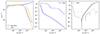 |
Fig. A.3. Hall individual conductivities profiles. The solid lines correspond to the solid grain case (γgrain = 190 erg cm−2) and the dashed lines to the fragile grain case (γgrain = 10 erg cm−2). The third panel displays the total Hall conductivity, taken as the sum of the different contributions, where the dotted parts are the negative values and the solid parts the positive ones. The solid grain case appears in black while the fragile case appears in grey. |
where md, τd, nion, μion and τion are respectively the dust mass and reduced temperature, the ion density, mean ion molecular weight and reduced temperature.  is the dust number distribution taken as a power law of index q and
  is a normalisation factor with smax and smin being the uppermost and lowermost sizes of the dust distribution considered. Integrating for any q < 4, we get:
![$$ \begin{aligned} n_{\rm ion} > \left\{ \begin{array}{ll} {\frac{K \left(n_{\rm H},T \right)}{s_{\rm max}} log \left(\frac{s_{\rm max}}{s_{\rm min}} \right), \mathrm{if~q} = 3} \\ {\frac{K \left(n_{\rm H},T \right)}{s_{\rm max}^{4-q}} \frac{4-q}{3-q} \left[s_{\rm max}^{-q+3}-s_{\rm min}^{-q+3} \right], \mathrm{otherwise}.} \end{array}\right. \end{aligned} $$](/articles/aa/full_html/2024/10/aa48268-23/aa48268-23-eq67.gif)
Here,  is a factor which depends on the gas density and the temperature. Considering
  , we can simplify the expressions to:
We can see that in reducing smin, the dust contribution would be more important and, thus, the ion density would have to be higher in order to maintain the dominance of the ion contribution. In increasing smax, for a given q and smin, we reduce the number of small grains and consequently relax the constrain on nion which can afford to be lower. We stress that to apply this equation at some density nH, one has to describe precisely the dust distribution, that is to know smax, smin and q. To gain insight, we apply Eq. (A.3) at the initial conditions of the collapse for which the shape of the distribution is known, since it is set as an MRN-like power law. With smin = 5 nm, smax = 250 nm, q = 3.5, nH = 2.6 × 106 cm−3 and T = 10 K, we get nion > 1.67 cm−3, and we can see on the various plots that initially nion ∼ 10−2 cm−3, which means it is indeed the dust contribution which prevails in regard to the perpendicular conductivity at that particular moment.
When it comes to the Hall conductivity, the individual ion conductivity yields negative values while those of the electrons and the dust yield positive values. Thus, there is a balance of power between the two groups in regard to the sign of the total Hall conductivity. At low densities, the electronic and ionic values are very close to each other, the ion conductivity being slightly superior. The dust contribution is only one order of magnitude lower but yet insufficient to reverse the trend directly. However, at some point during the collapse, the electron curve gets over the ion curve, resulting in the total Hall conductivity switching from negative to positive sign. Upon comparison with the ion conductivity, the electron conductivity is more strongly influenced by the population of small grains and since both conductivities are very close to each other throughout the collapse, the least variation in the population of small grains can affect the electronic capture and thus induce a change of sign of the Hall conductivity. That is why the Hall conductivity and thus the Hall resistivity are very sensitive to the overall dust distribution, large grains included. For instance, if the fragmentation threshold is shifted towards higher sizes, more massive grains can survive collisional events, and as a consequence the mass available for the repleshishment of small grains is lower. On the first panel, when fragmentation is curtailed (solid line), the small grains are significantly depleted, allowing the electron conductivity to dwell on large values. Initially, the ion conductivity is above the electronic one but gets beneath it and ends up sinking, yielding an early transition in the total Hall conductivity sign, slightly below nH = 109 cm−3. Nevertheless when considering fragile grains (dashed line), the early fragmentation triggers a significant replenishment of the small grains, resulting in a electronic conductivity decreasing and remaining below the ion conductivity until nH = 1010 cm−3 where the electrons take over. That is why the first transition occurs slightly later. Thereafter, the ion contribution recovers dominance slightly prior to nH = 1012 cm−3 to finally let the electron contribution prevail again at the end of the collapse. In this situation, the transition occurs three times during the collapse.
Appendix B: Comparison between fixed MRN and coagulating distribution with and without fragmentation
In Fig. B.2, we offer a simple comparison of the coagulation and fragmentation algorithms with other works. We use the same nomenclature as in Lebreuilly et al. (2023) to facilitate comparison. PC0 refers to the MRN non-evolving dust model, PC1 to the coagulating dust model and PC1 − FRAG to the coagulating plus fragmenting dust model. PC stands for protostellar collapse. It shows results similar to those in Lebreuilly et al. (2023) and Kawasaki et al. (2022). Note that for the sake of relevancy, in this peculiar case, we used the same value for the surface energy as the authors, namely, γbare, si = 25 erg cm−2, along with the appropriate reduced elastic modulus value for bare-silicate grains. In particular, we can clearly see the replenishment of small grains in PC1 − FRAG as compared with PC1, when fragmentation is included. This leads to a depletion of electrons at the latest stages of the collapse, and consequently to a change in the slopes of the ohmic and ambipolar resistivities.
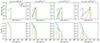 |
Fig. B.1. Dust distributions at different stages during the collapse. Comparison between the MRN non-evolving dust (PC0), the coagulation only (PC1), and the coagulation-fragmentaion (PC1 − FRAG) models. Top panels: Mass dust-to-gas ratio. Bottom panels: Number dust-to-gas ratio. |
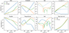 |
Fig. B.2. Conductivities and resistivities at different stages during the collapse (Hall resistivity : dotted line for the negative values and solid line for the positive ones). Comparison between the MRN non-evolving (PC0), the coagulation only (PC1), and the coagulation-fragmentaion (PC1 − FRAG) dust models. Last column: Electrons (solid) and ions (dashed) density (top), and peak size of the dust distribution (bottom). |
Appendix C: Considering the most efficient source of relative velocity for the removal of small grains
Figure C.1 provides a comparison of the effect of the different sources of grain collisions on the removal of small grains. TURB − COAG model includes only turbulence as a source of grain collisions. TURB − BR − COAG includes additionally Brownian motion while TURB − AD − COAG contains ambipolar diffusion. The models displaying FRAG account for fragmentation in addition to coagulation. We see that in the case of pure coagulation, the number of small grains is much lower when ambipolar diffusion is included, while it remains higher when only brownian motion is accounted for, at all densities. Therefore, in this context, ambipolar diffusion is the main process in regard to the depletion of small grains. However when including fragmentation, it seems that the gap in small grain removal efficiency between ambipolar diffusion and brownian motion is clearly reduced as fragmentation allows for a systematic replenishment of the small grains. At intermediate densities, ambipolar diffusion still appears to be slightly more efficient at removing the small grains, whereas at high density (last column), both velocity sources are contributing to the depletion of small grains with Brownian motion being slightly more efficient. Note that since TURB − AD − FRAG, TURB − BR − FRAG, and TURB − FRAG curves are not completely overlapping, small grain depletion is not completely suppressed by the repopulation induced by fragmentation. In addition, although there exists a striking difference in small grain population between models that include ambipolar diffusion and those which do not, we still observe a reduction of a few orders of magnitude in the overall number of small grains during the collapse (even more striking when fragmentation is off) regardless of the velocity source at play. Consequently, we can see on Fig. C.2 that even without ambipolar drift, the ambipolar resistivity, ηAD, reaches values larger than the MRN case.
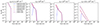 |
Fig. C.1. Dust number distributions at different stages during the collapse. Comparison between different sources of relative velocities with and without fragmentation : TURB (turbulence only), TURB − AD (turbulence plus ambipolar diffusion) and TURB − BR (turbulence plus Brownian motion). The solid lines refer to the purely coagulating cases, while fragmentation is included for the dashed lines (γgrain = 10 erg cm−2). |
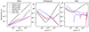 |
Fig. C.2. Magnetic resistivities at different stages during the collapse. Comparison between different sources of relative velocities with and without fragmentation : TURB (turbulence only), TURB − AD (turbulence plus ambipolar diffusion) and TURB − BR (turbulence plus brownian motion). The solid lines refer to the purely coagulating cases, while fragmentation is included for the dashed lines. The dashed black lines represent the non-evolving MRN dust distribution case. |
Appendix D: Ambipolar drift intensity in a collapsing core
Here is a map of the ambipolar drift intensity δAD in a collapsing core extracted from a 3D RAMSES (Teyssier 2002) simulation performed by Lebreuilly et al. (2020), with the mmMRNmhd model, at t = 80 Kyr (Fig. D.1). It is inferred by measuring the Lorentz force (∇×B) × B and comparing it with the approximation  (see Eq. 4). As clearly seen, the intermediate value δAD = 1 is scarce, while both larger and lower values are ubiquitous. In the most central region (very young, nascent protoplanetary disc and core), and at large scale in the pseudo-disc, the ambipolar drift intensity dwells around δAD = 10. Consequently, grain-grain erosion is expected to induce a significant replenishment of the population of small grains in those denser regions. In contrast, the ambipolar drift intensity is much weaker (δAD ∼ 0.1) in the rest of the domain, which hints at an inhibition of small grain coagulation via electrostatic repulsion in those diffuse regions. This reinforces the fundamental role that both mechanisms, electrosatic repulsion and grain-grain erosion, play in maintaining a reasonable ambipolar resistivity, ηAD, during the protostellar collapse.
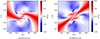 |
Fig. D.1. Face-on (left) and edge-on (right) slices of the ambipolar drift intensity, δAD, extracted from a non-ideal MHD collapse model (mmMRNmhd, Lebreuilly et al. 2020) computed with RAMSES (Teyssier 2002) at t = 80 Kyr. |
Appendix E: Impact of grain-grain erosion and electrostatic repulsion on the Ohm resistivity
Similarly to the analysis carried out in Sect. 4.2.2, we investigated the impact of grain-grain electrostatic repulsion and erosion on the Ohm resistivity η0 for different values of the ambipolar drift intensity δAD. Looking at the first column, we can see that contrary to the ambipolar resistivity, the Ohm resistivity remains almost unaffected at all densities even for a weak ambipolar drift intensity (δAD = 0.1) for which electrostatic repulsion is expected to significantly inhibit small grains coagulation. While the dust contributes directly to the ambipolar resistivity, ηAD, at low density (any change in the small grain population is reflected almost immediately in the resistivity profile), it only acts indirectly on the ohmic resistivity, via electron capture. At low densities, the cross-section for electron capture is very low and only a sufficient abundance of small grains, such as the one enabled by a lower sticking efficiency (ϵstick = 0.5, bottom left panel), allows for an efficient collection of electrons and, thus, a rise in the ohmic resistivity. At high density, the grain collisional velocities are usually above the Coulomb velocity threshold (Eq. 18), thereby suppressing the effect of electrostatic repulsion.
When it comes to the impact of erosion (right column), it is clear that for low and intermediate values of ambipolar drift intensity (δAD = 0.1 and δAD = 1), the collisional velocities are not high enough to induce a sufficient replenishment of small grains prior to nH = 1012 cm−3. However, beyond this density, the collisional velocities and dust size ratios sratio (see Eq. 17) are large enough to enhance the erosion efficiency and thus to allow for the excess of small grains to efficiently capture the electrons and to allow for a soaring in terms of the Ohm resistivity. Nevertheless, in order to increase the resistivity at lower density, we need to rely on a stronger ambipolar drift intensity δAD = 10, as seen by looking at the purple dotted curve. We note that for δAD = 0.1 and δAD = 1, a sticking efficiency of ϵstick = 0.5 does reduce the small grain coagulation rate, but is also detrimential to erosion, since only half of the collisions are destructive. This results in an overall suppression of the late rise in ohmic resistivity.
In any case, the Ohm resistivity remains at least two orders of magnitude below the MRN reference because no process is capable of completely making up for the very short coagulation timescales. Besides, it remains dominated by the ambipolar resistivity ηAD at least up to the final density value of our simulations, namely, nH = 2 × 1013 cm−3.
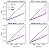 |
Fig. E.1. Ohm resistivity, ηO, evolution during the protostellar collapse for different values of the ambipolar drift intensity or equivalently different ambipolar drift velocities: δAD = 0.1 (0.1VAD), δAD = 1 (VAD), and δAD = 10 (10VAD). Grain-grain electrostatic repulsion (first column) and erosion (second column) are also included (dotted lines). Second row: Same, but with a sticking efficiency of 0.5. |
Appendix F: Impact of the grain-grain sticking efficiency, ϵstick
Here, we vary the sticking efficiency of grains, ϵstick, (included in our coagulation algorithm) and explore its impact on the evolution of the dust distribution as well as on the magnetic resistivities. We note that ϵstick = 0.5 implies that half of the collisions result in bouncing rather than coagulation or fragmentation, namely, that both grains remain intact. Figure F.1 indicates that a value of 0.1, which would significantly hinder the small grains coagulation at low density, allowing us to recover the MRN resistivities to some extent. We note that a value of 0.1 means that only one collision out of ten leads to grain sticking, thus leading to coagulation. A value of 0.3 slows down the coagulation process (as readily seen on the ambipolar resistivity ηAD profile) and allows for the ambipolar resistivity to be notably reduced prior to nH = 109 cm−3. However, for values beyond ϵstick = 0.5, no significant changes are induced. This parameter also has a clear impact on the peak size of the dust distribution. Indeed, a lower sticking efficiency implies a longer coagulation timescale and, consequently, a reduced dust peak size.
All Tables
All Figures
|
Fig. 1. Gas numerical density evolution with time throughout the gravitational collapse. |
| In the text | |
|
Fig. 2. Dust distributions at different stages during the collapse. First row: Mass dust-to-gas ratio. Second row: Number dust-to-gas ratio. Third row: Resistivities profile and ion and electron numerical densities (Hall resistivity: dotted line for the negative values and solid line for the positive ones). Dashed black lines: Reference resistivities obtained with a fixed MRN dust distribution. Fourth row: Parallel, perpendicular, and Hall conductivities, and the evolution of the peak size of the dust distribution. Comparison between different values of the grain surface energy expressed in cgs units (erg cm−2). |
| In the text | |
|
Fig. 3. Same as Fig. 2, but investigating the influence of grain-grain erosion with γgrain = 190 erg cm−2. |
| In the text | |
|
Fig. 4. Ambipolar resistivity ηAD evolution during the protostellar collapse for different values of the ambipolar drift intensity or equivalently different ambipolar drift velocities: δAD = 0.1 (0.1VAD), δAD = 1 (VAD), and δAD = 10 (10VAD). Grain-grain electrostatic repulsion (first column) and erosion (second column) are also included (dotted lines). Second row: Same details, but with a sticking efficiency of 0.5. |
| In the text | |
|
Fig. 5. Ambipolar resistivity, ηAD, (normalized with the squared initial magnetic field strength) evolution with gas density throughout the protostellar collapse, for different values of the initial magnetic field strength. Solid lines: growing dust distribution (γgrain = 190 erg cm−2). Dashed lines: non evolving MRN dust distribution. Dotted red line is the analytical dust-free solution. |
| In the text | |
|
Fig. 6. Freefall timescale (in black) and ambipolar diffusion timescale as a function of gas density throughout the protostellar collapse for different values of the ambipolar drift intensity. The dashed grey line represents the fixed MRN case. The solid lines correspond to resistant grains (γgrain = 190 erg cm−2) whereas the dotted lines correspond to the fragile grains (γgrain = 10 erg cm−2). |
| In the text | |
|
Fig. 7. Freefall timescale (in black) and ambipolar diffusion timescale as a function of gas density throughout the protostellar collapse for different values of the ionisation rate induced by cosmic rays. The initial magnetic field chosen corresponds to the critical value (minimum value) above which the small grain depletion leads to an ambipolar diffusion timescale lower than the freefall timescale. |
| In the text | |
|
Fig. A.1. Individual conductivities profiles. The third panel displays the parallel conductivity. The solid lines correspond to the solid grain case (γgrain = 190 erg cm−2) and the dashed lines to the fragile grain case (γgrain = 10 erg cm−2). |
| In the text | |
|
Fig. A.2. Perpendicular individual conductivities profiles. The third panel displays the total perpendicular conductivity, taken as the sum of the different contributions. The solid lines correspond to the solid grain case (γgrain = 190 erg cm−2) and the dashed lines to the fragile grain case (γgrain = 10 erg cm−2). |
| In the text | |
|
Fig. A.3. Hall individual conductivities profiles. The solid lines correspond to the solid grain case (γgrain = 190 erg cm−2) and the dashed lines to the fragile grain case (γgrain = 10 erg cm−2). The third panel displays the total Hall conductivity, taken as the sum of the different contributions, where the dotted parts are the negative values and the solid parts the positive ones. The solid grain case appears in black while the fragile case appears in grey. |
| In the text | |
|
Fig. B.1. Dust distributions at different stages during the collapse. Comparison between the MRN non-evolving dust (PC0), the coagulation only (PC1), and the coagulation-fragmentaion (PC1 − FRAG) models. Top panels: Mass dust-to-gas ratio. Bottom panels: Number dust-to-gas ratio. |
| In the text | |
|
Fig. B.2. Conductivities and resistivities at different stages during the collapse (Hall resistivity : dotted line for the negative values and solid line for the positive ones). Comparison between the MRN non-evolving (PC0), the coagulation only (PC1), and the coagulation-fragmentaion (PC1 − FRAG) dust models. Last column: Electrons (solid) and ions (dashed) density (top), and peak size of the dust distribution (bottom). |
| In the text | |
|
Fig. C.1. Dust number distributions at different stages during the collapse. Comparison between different sources of relative velocities with and without fragmentation : TURB (turbulence only), TURB − AD (turbulence plus ambipolar diffusion) and TURB − BR (turbulence plus Brownian motion). The solid lines refer to the purely coagulating cases, while fragmentation is included for the dashed lines (γgrain = 10 erg cm−2). |
| In the text | |
|
Fig. C.2. Magnetic resistivities at different stages during the collapse. Comparison between different sources of relative velocities with and without fragmentation : TURB (turbulence only), TURB − AD (turbulence plus ambipolar diffusion) and TURB − BR (turbulence plus brownian motion). The solid lines refer to the purely coagulating cases, while fragmentation is included for the dashed lines. The dashed black lines represent the non-evolving MRN dust distribution case. |
| In the text | |
|
Fig. D.1. Face-on (left) and edge-on (right) slices of the ambipolar drift intensity, δAD, extracted from a non-ideal MHD collapse model (mmMRNmhd, Lebreuilly et al. 2020) computed with RAMSES (Teyssier 2002) at t = 80 Kyr. |
| In the text | |
|
Fig. E.1. Ohm resistivity, ηO, evolution during the protostellar collapse for different values of the ambipolar drift intensity or equivalently different ambipolar drift velocities: δAD = 0.1 (0.1VAD), δAD = 1 (VAD), and δAD = 10 (10VAD). Grain-grain electrostatic repulsion (first column) and erosion (second column) are also included (dotted lines). Second row: Same, but with a sticking efficiency of 0.5. |
| In the text | |
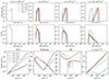 |
Fig. F.1. Same as Fig. 2, but investigating the grain sticking efficiency (γgrain = 190 erg cm−2). |
| In the text | |
Current usage metrics show cumulative count of Article Views (full-text article views including HTML views, PDF and ePub downloads, according to the available data) and Abstracts Views on Vision4Press platform.
Data correspond to usage on the plateform after 2015. The current usage metrics is available 48-96 hours after online publication and is updated daily on week days.
Initial download of the metrics may take a while.