| Issue |
A&A
Volume 683, March 2024
|
|
|---|---|---|
| Article Number | A91 | |
| Number of page(s) | 9 | |
| Section | Cosmology (including clusters of galaxies) | |
| DOI | https://doi.org/10.1051/0004-6361/202245798 | |
| Published online | 08 March 2024 | |
Testing the spatial geometry of the Universe with TianQin: Prospect of using supermassive black hole binaries
1
School of Science, Chongqing University of Posts and Telecommunications, Chongqing 400065, PR China
2
Department of Physics and Chongqing Key Laboratory for Strongly Coupled Physics, Chongqing University, Chongqing 401331, PR China
3
Department of Physics, College of Sciences, Northeastern University, Shenyang 110004, PR China
4
Department of physics, Chongqing University, 400044 Chongqing, PR China
e-mail: cqujinli1983@cqu.edu.cn
5
Institute for Frontiers in Astronomy and Astrophysics, Beijing Normal University, Beijing 102206, PR China
e-mail: caoshuo@bnu.edu.cn
6
Department of Astronomy, Beijing Normal University, Beijing 100875, PR China
7
School of Physics and Astronomy, China West Normal University, Nanchong 637009, PR China
e-mail: qqjiangphys@yeah.net
Received:
25
December
2022
Accepted:
21
October
2023
Context. The determination of the spatial geometry of the Universe plays an important role in modern cosmology. Any deviation from the cosmic curvature ΩK = 0 would have a profound impact on the primordial inflation paradigm and fundamental physics.
Aims. In this paper, we carry out a systematic study of the prospect of measuring the cosmic curvature with the inspiral signal of supermassive black hole binaries (SMBHBs) that could be detected with TianQin.
Methods. The study is based on a method that is independent of cosmological models. It extended the application of gravitational wave (GW) standard sirens in cosmology. By comparing the distances from future simulated GW events and simulated H(z) data, we evaluated whether TianQin produced robust constraints on the cosmic curvature parameter Ωk. More specifically, we considered three-year to ten-year observations of supermassive black hole binaries with total masses ranging from 103 M⊙ to 107 M⊙.
Results. Our results show that in the future, with the synergy of ten-year high-quality observations, we can tightly constrain the curvature parameter at the level of 1σ Ωk = −0.002 ± 0.061. Moreover, our findings indicate that the total mass of SMBHB does influence the estimation of cosmic curvature, as implied by the analysis performed on different subsamples of gravitational wave data.
Conclusions. Therefore, TianQin is expected to provide a more powerful and competitive probe of the spatial geometry of the Universe, compared to future spaced-based detectors such as DECIGO.
Key words: gravitation / gravitational waves
© The Authors 2024
 Open Access article, published by EDP Sciences, under the terms of the Creative Commons Attribution License (https://creativecommons.org/licenses/by/4.0), which permits unrestricted use, distribution, and reproduction in any medium, provided the original work is properly cited.
This article is published in open access under the Subscribe to Open model. Subscribe to A&A to support open access publication.
1. Introduction
As a successful gravity theory in which general coordinate invariance plays an essential role, Einstein’s theory of General Relativity (GR) has passed all observational test so far, ranging from submillimeter (Li et al. 2003, 2008) to galactic scales (Cao et al. 2017). In recent years, the appearance of gravitational waves (GWs) has provided us with a new window for studying cosmology. Prior to the detection of GWs, all cosmological parameter inferences were made using electromagnetic (EM) radiation from extragalactic sources. Currently, we can detect GWs produced by inspiraling binary systems that provide absolute distance information (Schutz 1986). Therefore, we can use these binary systems as standard sirens. Gravitational waves have been applied in various ways in cosmology (Zhao et al. 2011; Cai & Yang 2017; Liao 2019a,b; Liao et al. 2017a, 2022; He et al. 2022; Pan et al. 2021; Zhang et al. 2023).
Fortunately, since the successful detection of the first GW event by the advanced Laser Interferometer Gravitational-Wave Observatory (LIGO) (GW150914; Abbott et al. 2016a,b,c,d, 2017a,b, c), several GW events from mergers of binary black holes (Abbott et al. 2016c,d) and one GW event that was accompanied by an electromagnetic counterpart from the merger of binary neutron stars have been observed (Abbott et al. 2018, 2020). Furthermore, GWs are helpful for exploring some extreme conditions, such as the very early Universe, extremely high energy scales, and additional dimensions. The detection of GWs therefore received considerable attention (Petiteau et al. 2011). New generations of GW detectors have been proposed to cover different frequency bands. With these detectors, more binary coalescences are expected to be detected at longer distances, and they have higher a signal-to-noise ratio (S/N). These sources are very important for us to study the evolution of universe (Petiteau et al. 2011). At present, the gravitational wave detection projects promoted both at home and abroad include ground-based and space-based GW detectors. The ground-based GW detectors include the LIGO and Virgo observatories, and the Kamioka Gravitational Wave Detector (KAGRA) and Einstein Telescope (ET) GW detectors. The space-based projects include the Laser Interferometer Space Antenna (LISA), DECi-hertz Interferometer Gravitational wave Observatory (DECIGO), and two Chinese detectors, TianQin (TQ) and Taiji (Gong et al. 2021). Space-based detectors can detect GWs below 1Hz, but ground-based detectors cannot, because they are affected by terrestrial gravity gradient noise. The TQ Project, first proposed by Sun Yat-sen University in China in 2014, is a space-based gravitational wave detector with some features. It is capable of detecting GWs in the range of 10−4–10−1 Hz to fill the gap between DECIGO and LISA. In addition, the equilateral triangle arm of TQ is around 105 km. Because of the shorter arm and better sensitivity compared with LISA in the higher-frequency regime, it might perform better than LISA (Gong et al. 2021). There are three steps for the TQ project. The successful launch of the TQ-1 satellite in 2019 has achieved all mission objectives, which is the main objective in the first step of the project. The main goal of the second step of the project is to launch two satellites in 2025. TQ-2 would be able to detect GWs if laser phase noise does not affect it. The third step of the project, which is expected to take place in 2035, aims to ensure that the three satellites operate smoothly in geocentric orbit and can successfully detect GWs, but this is subject to the successful implementation of the first two steps. The TQ GW detector can observe GW signals, including those from SMBHBs, stellar mass binary black hole mergers (SBBH), and extreme mass-ratio inspirals (EMRIs; Zhu et al. 2022).
Many studies have been made of SMBHBs. For example, Feng et al. (2019) used the Fisher information matrix to estimate the parameter precision of SMBHBs for TQ. They found that the parameters of SMBHBs could be determined with a high precision, which means that the SMBHBs are the most powerful GW sources detected by TQ. In addition, the spatial curvature of the universe is one of the most important problems in cosmology. Its importance stems from the following three aspects. Firstly, the estimation of cosmic curvature parameter could provide an important probe of the well-known Friedman – Lemaître – Robertson – Walker (FLRW) metric (Cao et al. 2019; Qi et al. 2019). Secondly, the cosmic curvature is closely related to the evolution of the Universe and the hypostasis of dark energy (DE). Even a very small curvature of the Universe has a very strong effect on the reconstruction of the DE equation of state (Clarkson et al. 2007; Gong & Wang 2007; Virey et al. 2008; Ichikawa et al. 2006). Moreover, the failure of the FLRW approximation might provide an explanation of the accelerating expansion in the late-time Universe (Ferrer & Rasanen 2006; Enqvist 2008; Ferrer et al. 2009; Rasanen 2009; Boehm & Räsänen 2013; Lavinto et al. 2013; Redlich et al. 2014). Therefore, it is necessary to constrain the cosmic curvature from popular observational probes, and this has indeed been extensively studied in the literature (Zhao et al. 2007; Wright 2007; Wei & Wu 2017; Li et al. 2016). In this work, we investigate the potential of constraining the cosmic curvature with SMBHBs covering the total mass range of 103 − 107 M⊙.
Generally, three theoretical methods can be used to constrain the spatial curvature of the Universe. One is the model-dependent method using the photometric distance expressed by the cosmological constant model, which does not directly measure the cosmic curvature geometrically. Another approach is the model-independent method based on the zero geodesic distance of the FLRW metric to constrain the spatial curvature (Bernstein 2006; Liao et al. 2017b; Qi et al. 2018; Denissenya et al. 2018). The third model-independent method was proposed to constrain Ωk from the measurements of the expansion rate (H(z)), the comoving distance (D(z)), and its derivative with respect to z (Clarkson et al. 2007):  . At present, many works have used this method to constrain the cosmic curvature based on the observations of different types of cosmological distances (Shafieloo & Clarkson 2010; Cao et al. 2017; Cai et al. 2016; Sapone et al. 2014; Li et al. 2014). However, the first derivative of D′(z) must be estimated, which may bring a large uncertainty to the final estimation of ΩK. In this work, we study the potential of an improved method that is independent of a cosmological model and that extended the application of gravitational wave standard sirens in cosmology, based on the inspiral signal of supermassive black hole binaries that could be detected with TQ. In the framework of this method, Wei & Wu (2017) proposed the Gaussian process (GP) method to constrain the cosmic curvature by combining the most recent Hubble parameter H(z) and supernova Ia data, which turned out to agree with zero cosmic curvature. By comparing the distances from future simulated GW events and current CC Hubble data, Wei (2018) continued to expand the application of GW standard sirens in measuring cosmic curvature. They simulated hundreds of GW data sets from ET to constrain the curvature parameter and obtained a result with higher precision, for which Ωk = −0.002 ± 0.028. More recently, He et al. (2022) reconstructed the Hubble parameters without the influence of the hypothetical model, and combined it with DECIGO GW data to obtain a high-precision result (Ωk = −0.07 ± 0.016).
The paper is organized as follows. The simulation of the TianQin data is introduced in Sect. 2. The method and corresponding constraints on cosmic curvature from the TQ are presented in Sect. 3. The final discussion and conclusions are summarized in Sect. 4.
2. Observational data
In this section, we briefly introduce the method we employed to simulate observations of GW standard sirens from the TQ. In the following simulations, we adopt the flat ΛCDM with the Hubble constant H0 = 69.6 km s−1 Mpc−1 with a 1% uncertainty and the matter density parameter Ωm = 0.286 (Bennett et al. 2014).
As a typical millihertz frequency gravitational wave observatory, TQ is designed to mainly detect GWs from Galactic ultra-compact binaries, coalescing SMBHBs, EMRIs, and the inspiral of an SBBH (Hughes 2001; Sesana 2016; Di & Gong 2018; Olmez et al. 2010). The SMBHB mergers are considered to be the most powerful GW sources that could be observed by TQ (Feng et al. 2019). Therefore, we simulated GW data sets of SMBHBs for three, five, and ten years according to the continuous observation time of TQ in the future. For the data of each year, the masses ranged from 103 M⊙ to 107 M⊙, and we split the data sets into three subsamples according to the mass range of SMBHBs (TQ103 ∼ 104 M⊙, TQ104 ∼ 105 M⊙, TQ105 ∼ 106 M⊙, and TQ106 ∼ 107 M⊙). For each subsample, the redshift z is chosen in the range of 0 ∼ 2.5. Moreover, for the event rate of SMBHBs that TianQin can detect each year, we refer to the recent results based on the popIII model, which assumes low-mass black hole seeds from popIII stars and accounts for the delays between massive black hole and galaxy mergers (Yi et al. 2022). In Fig. 1 we present the event rates for different mass intervals and redshift intervals, the distribution of which agrees well with that of Klein et al. (2016). It should be noted that because TQ has two observation windows of two and three months each year (Luo et al. 2016), the practically detected SMBHB event is only half of the predicted number proposed in Yi et al. (2022).
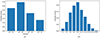 |
Fig. 1. Event rates for different mass ranges (left panel) and redshift ranges (right panel) based on the popIII model. |
It is well known that the absolute measurements of the luminosity distance DL to the source and the chirp mass Mc can be determined from the chirping signals of GW (Schutz 1986). In addition, the chirp mass can be measured by the phase of the GW signal, and DL can thus be extracted from the strain amplitude of GW. For the waveform of GW, we chose ℋ(f) in stationary-phase approximation,
![$$ \begin{aligned} \mathcal{H} (f)=Bf^{-7/6}\exp [i(2\pi ft_0-\pi /4+2\psi (f/2)-\varphi _{(2.0)})], \end{aligned} $$](/articles/aa/full_html/2024/03/aa45798-22/aa45798-22-eq2.gif)
where B is the Fourier amplitude, and
where  is the chirp mass (see Feng et al. 2019 for the expression of F+, F× and phase parameters for advanced TQ). In addition, DL is the luminosity distance, and in the standard flat ΛCDM cosmological model, it can be expressed as
The one-sided power spectral density (PSD) of the noise in TQ is (Feng et al. 2019)
where Sx = 10−24 m2 Hz−1 denotes the PSDs of the position noise, L = 1.73 × 10⁵ km denotes the arm length, and Sa = 10−30 m2 s−4 Hz−1 denotes the PSDs of residual acceleration noise. Correspondingly, the S/N of TQ can be calculated as
where ffin = min(fISCO, fend) and the fISCO = c3/(63/2MGπ) Hz is the GW frequency at the innermost stable circular orbit, fend = 1 Hz is the upper cutoff frequency for TQ, fin = max(flow, fobs), with the lower cutoff frequency flow = 10−5 Hz and the initial observation frequency fobs = 4.15 × 10⁻⁵(Mc/106 M⊙)−5/8(Tobs/1 yr)−3/8 Hz.
Following the error strategy proposed in the literature (Sathyaprakash et al. 2010; Zhao et al. 2011), the total uncertainty of DL includes the contribution from the measurement itself  and an additional uncertainty
  due to weak lensing,
The luminosity distance and total error of GW data can be obtained by the above process. Then we can test the spatial flatness of the Universe in a way that does not depend on a cosmological model using the GW data.
3. Method and constraints on cosmic curvature
3.1. The GP method
The GP method (Seikel et al. 2012; Wu et al. 2020; Liu et al. 2019; Liao et al. 2019, 2020) is a non-parametric smoothing method for reconstructing functions, which does not need to consider the influence of other cosmological background models when placing limits on cosmic curvature. In particular, the distribution of DL(z) with redshift is directly obtained by GP method from H(z) observations. We reconstructed the function E(z) from the H(z) data using the GP method based on the Gapp code, which has been widely used in cosmological studies (Wu et al. 2020; Liu et al. 2019), and the H(z) data were taken from Table 1 of Wei & Wu (2017). The advantage of this method is that we can derive a model-independent function E(z) without any prior assumption on the cosmological models (Seikel et al. 2012; Cao et al. 2011, 2015; Cao & Liang 2013). Through the data analysis, the H(z) can be obtained in two ways: by calculating the passively evolving galaxy ages, and by detecting radial BAO features. We show the data in Table 1 (Jimenez et al. 2003; Simon et al. 2005; Stern et al. 2010; Chuang & Wang 2012; Moresco et al. 2012, 2016; Zhang et al. 2014; Moresco 2015; Gaztanaga et al. 2009; Blake et al. 2012; Samushia et al. 2013). Because the proper distance dP depends on the E(z) function, we can use the H(z) measurements to reconstruct the E(z) function and then derive dP from the function E(z). The details of the steps to reconstruct the function are as follows: firstly, we normalize the H(z) function and their 2σ errors based on the H(z) data points with the GP method. Secondly, the reconstructed function E(z) can be obtained according to the E(z) = H(z)/H0 relation, where H0 = 69.6 ± 0.7 km s−1 Mpc−1 (Bennett et al. 2014). Thirdly, the proper distance dP with their 2σ errors can be obtained through the reconstructed function E(z) using this formula:  . As is shown in Fig. 2, the observed (blue points) and reconstructed (solid red lines) H(z) are well consistent with those determined from the best-fit flat ΛCDM model (solid blue lines). The reconstruction of the dP(z) function based on the H(z) sample is also presented in Fig. 2.
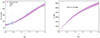 |
Fig. 2. Reconstructed H(z) and dp(z) function from the GP method using the H(z) data with H0 = 69.6 ± 0.7 km s−1 Mpc−1. The H(z) observational data and the ΛCDM model are also added for comparison. |
H(z) data measurement from the differential age method (I) and the radial BAO method (II).
3.2. Observational constraints on Ωk
We adopted the χ2 minimum fitting method and the Markov chain Monte Carlo (MCMC) technique to constrain the cosmic curvature Ωk based on the following expression:
![$$ \begin{aligned} \frac{D_{\rm L}(z)}{(1+z)} = \left\{ \begin{array}{lll} \frac{c}{H_{0}}\frac{1}{\sqrt{|\Omega _{k}|}}\sinh \left[\sqrt{|\Omega _{k}|}d_{\rm P}(z)\frac{H_{0}}{c}\right]\,\,\mathrm{for}\,\,\Omega _{k}>0\\ d_{\rm P}(z)\quad \mathrm{for}\,\,\Omega _{k}=0, \\ \frac{c}{H_{0}}\frac{1}{\sqrt{|\Omega _{k}|}}\sin \left[\sqrt{|\Omega _{k}|}d_{\rm P}(z)\frac{H_{0}}{c}\right]\,\,\mathrm{for}\,\,\Omega _{k} < 0\\ \end{array} \right. \end{aligned} $$](/articles/aa/full_html/2024/03/aa45798-22/aa45798-22-eq13.gif)
where Ωk is the spatial curvature, and dp is the proper distance that can be reconstructed with the GP method using H(z) data. The corresponding error can be expressed as
![$$ \begin{aligned} \sigma _{D_{\rm L}} = \left\{ \begin{array}{lll} (1+z)\cosh \left[\sqrt{|\Omega _{k}|}d_{\rm P}(z)\frac{H_{0}}{c}\right]\sigma _{d_{\rm P}}\,\,\mathrm{for}\,\,\Omega _{k}>0\\ (1+z)\sigma _{d_{\rm P}}\quad \mathrm{for}\,\,\Omega _{k}=0, \\ (1+z)\cos \left[\sqrt{|\Omega _{k}|}d_{\rm P}(z)\frac{H_{0}}{c}\right]\sigma _{d_{\rm P}}\,\,\mathrm{for}\,\,\Omega _{k} < 0. \\ \end{array} \right. \end{aligned} $$](/articles/aa/full_html/2024/03/aa45798-22/aa45798-22-eq14.gif)
The χ2 can be written as
where N represents the total number of simulated GW data,  represents the observed luminosity distance, and the
  is the theoretical counterpart that can be obtained from Eq. (8).
In Fig. 3a we show the probability distribution of the spatial curvature based on the ten-year observation of TQ (103 ∼ 107 M⊙) and H(z) data. The best-fit curvature (Ωk) and its corresponding 1σ uncertainty are determined to be Ωk = 0.00 ± 0.19. Due to the limited number of TQ data simulated with the popIII model within the mass range of 103 ∼ 107 M⊙ and redshift range of 0 ∼ 2.5 (only 24 data points in ten years), this result cannot fully demonstrate the constraining effect of TQ GW data on curvature. Therefore, we simulated H(z) data to extend its upper redshift limit, thereby expanding the data set corresponding to TQ. We acknowledge that the measurement of the BAO scale in the line-of-sight direction enables the determination of the Hubble parameter H(z) at various redshifts. Consequently, Seo & Eisenstein (2007) employed even binning in ln(1 + z) to predict an all-sky survey within the redshift range of 0 ∼ 5. Building upon the work of Seo & Eisenstein (2007), Weinberg et al. (2013) used their fast-approximation method for the full Fisher matrix calculation to make predictions regarding H(z). This method takes the idealized treatment of acoustic oscillations, non-linear structure formation, and redshift–space distortions into account. By incorporating survey redshift, number density, and volume, the method enables precise forecasts of H(z) with an uncertainty of approximately 1%. Consequently, Yu & Wang (2016) performed simulations of H(z) data within the 0.1 ∼ 5 redshift range based on this approach, and constrained the cosmic curvature using a model-independent method. We refer to their work, and the specific process of simulating H(z) in this paper is as follows: We adopted a flat ΛCDM model with parameter values H0 = 69.6 km s−1 Mpc−1 and Ωm = 0.286. A total of 20 data points were generated, evenly distributed in the ln(1 + z) space, covering a redshift range of 0.1 ≥ z ≤ 5 (Yu & Wang 2016), and the uncertainty of these relevant data was 1% (Weinberg et al. 2013). Figure 4a shows the reconstruction results (solid red lines) of the simulated H(z) data (blue points) using the GP method, which are consistent with the flat ΛCDM model (solid blue line). Figure 4b illustrates the reconstructed dp(z) function based on the simulated H(z) data. At the same time, the redshift z range of 0 ∼ 5 was selected to simulate the TQ GW data again, following the same procedure as described in Sect. 2. Additionally, Fig. 5 presents the specific number distribution for each subsample simulated based on the popIII model, while Fig. 6 displays the distribution of redshift (z) and luminosity distance (DL) for the ten-year data.
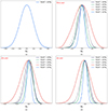 |
Fig. 3. 1D distribution of the cosmic curvature derived from different subsamples of SMBHBs. Panel a represents the result of H(z) data combined with ten-year observations of TQ, while panels b, c and d correspond to the results of simulated H(z) data combined with three-, five-, and ten-year observations of TQ, respectively. |
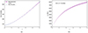 |
Fig. 4. Reconstructed H(z) and dp(z) functions with the GP method using the H(z) simulated data with H0 = 69.6 ± 0.7 km s−1 Mpc−1. The H(z) simulated data and the ΛCDM model are also added for comparison. |
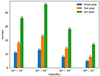 |
Fig. 5. Specific number of SMBHBs that TQ could detect. |
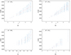 |
Fig. 6. Simulated gravitational wave data (DL − z relation) derived from different subsamples of SMBHBs (with total masses of TQ103 ∼ 107 M⊙) based on ten-year observations of TQ. |
Figures 3b,c, and d show the probability distribution of the spatial curvature based on the simulated H(z) data and the three-, five- and ten-year observations of TQ, respectively. Table 2 presents the best-fit curvature (Ωk) and the corresponding 1σ uncertainties obtained from different subsamples. The table shows that when the GW source total mass is different, the results obtained by using ten-year data are −0.02 ± 0.13(103 ∼ 104 M⊙), −0.014 ± 0.097(104 ∼ 105 M⊙), −0.01 ± 0.12(105 ∼ 106 M⊙), and −0.06 ± 0.2(106 ∼ 107 M⊙), respectively. In addition, we combined the 103 M⊙ ∼ 107 M⊙ data and the constraint on the parameter is −0.002 ± 0.061. These results all include Ωk = 0 within the 1σ uncertainties, which means that our Universe is spatially flat. Ωk = 0 is also included in the 1σ uncertainties for the results from three, and five year. Moreover, through the comparison of the analysis results in Fig. 7a, we find that for GW sources with the same mass, the precision of the cosmic curvature constraint would increase with the observation time. In Fig. 7b, we also present the variation of cosmic curvature precision with the total mass of GW sources. Our results demonstrate an obvious Ωk improvement when the total mass of GW source is 104 ∼ 105 M⊙. There are two possible explanations for this interesting tendency: (I) GW sources with masses of 104 ∼ 105 M⊙ dominate the full sample (as can be seen in Fig. 5), which leads to the most stringent limits on the cosmic curvature. (II) The differences of S/N in SMBHB subsamples covering different total masses might also affect the constraints on Ωk. In order to investigate these possibilities, a plot of the amplitudes of GW waveforms for SMBHBs with different mass ranges is shown in Fig. 8, along with the TianQin sensitivity curve at redshift z = 0.5, 1, 1.5 and 2. Our findings suggest that the SMBHB subsample with a total mass of 104 ∼ 105 M⊙ posses a very high sensitivity of detection in the framework of the TianQin detectors.
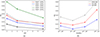 |
Fig. 7. Variation in the precision of Ωk with different observation times (left panel) and different total masses of the SMBHB (right panel). |
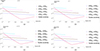 |
Fig. 8. Amplitude evolution for SMBHBs with different mass ranges at redshift z = 0.5, 1, 1.5, and 2. The sensitivity curve of the TQ is also added for comparison. |
Best-fit spatial curvature (Ωk) and the corresponding 1σ uncertainties derived from different subsamples of SMBHBs based on H(z) simulated (H(z)simulate) data and three-, five-, and ten-year observations of TQ.
In addition, in order to more intuitively reflect the constraint effect of TQ data on cosmic curvature, we compared the results obtained from other observation data constrained by the same method (Zhang et al. 2022; Cao et al. 2022; Wei 2018; Wei & Melia 2020a,b). The results are shown in Table 3. Firstly, the results given by the second-generation GW detector DECIGO and the third-generation GW detector ET are Ωk = −0.05 ± 0.12 and Ωk = 0.035 ± 0.039, respectively. Compared with DECIGO and ET constraint results, the precision of our result (Ωk = −0.002 ± 0.061) is improved by 49.2% and decreased by 56.4%, respectively. This indicates that the TQ is expected to provide a more powerful and competitive probe of the spatial geometry of the Universe compared to future space-based detectors such as DECIGO. However, combined with the DECIGO and Legacy Survey of Space and Time (LSST) strong-lense data, the result is Ωk = 0.0001 ± 0.012, and the precision of our result is reduced by a factor of 4.1 compared to this. In addition, we also show the results given by quasar (Ωk = −0.918 ± 0.429) and lensing+quasar+SNe ( ). The constraint precision of the TQ GW data is 85.8% and 59.3.3% higher than theirs, respectively. This means that the GW data have a better constraint effect on the cosmic curvature than electromagnetic wave data such as quasar, lenses, and SNe under this method. Finally, the precision of our results is reduced by a factor of 2.4 compared to the Planck 2018 results (△Ωk = 0.018; Planck Collaboration VI 2020).
Results of Ωk obtained with the GP method.
4. Conclusions
We investigated the spatial curvature of the Universe in a GP way, based on the GW observations from the future space-based GW detector TQ. For the distance measurement, we considered simulated data of GWs from SMBHBs, which can be considered as standard sirens covering different redshift ranges. For the non-parametric reconstruction of the distance and redshift relation, we used the H(z) data, based on the non-parametric smoothing method called GP, and the reconstructed function was independent of the model. Then we obtained the comoving distance dP(z) by directly solving the integral of this reconstructed function E(z). Furthermore, with the spatial curvature Ωk taken into consideration, we were able to transform the comoving distance into the DL. Then, we constrained Ωk using the MCMC method and the χ2 minimum fitting method. Our conclusions are listed below.
-
Firstly, the 1D distribution of cosmic curvature obtained by combining H(z) and TQ GW data is shown in Fig. 3a, and the result is Ωk = 0.00 ± 0.19. However, by analysing the data, we found that the obtained result failed to demonstrate the constraint effect of TQ GW data on curvature. Therefore, we increased the upper redshift limit by simulating H(z) data to obtain additional TQ GW data. The final results are presented in Figs. 3b,c, and d, along with the corresponding numerical estimations summarized in Table 2. Our results show that Ωk = −0.002 ± 0.061(1σ), by combining H(z) simulated data with simulated GW events of TQ, and this suggests that our Universe is flat.
-
In addition, according to the results in Table 2, it is found that the precision of Ωk constraint increases with increasing observation duration, and the total mass of the SMBHB does influence the estimation of cosmic curvature, as implied by the analysis performed on different subsamples of gravitational wave data.
-
Finally, compared to the previous model-independent constraints on the spatial curvature by GW data (DECIGO) (Zhang et al. 2022; Wei 2018), TQ is expected to provide a powerful and competitive probe of the spatial geometry of the Universe. The results are also available for the space-based GW detector Taiji, which will be sensitive in observing GWs from SMBHBs around 1 mHz.
Finally, through the analysis of the GW data from the SMBHB observed by future GW detectors, our studies provide a possible approach to testing the spatial properties of the Universe. Focusing on the strong degeneracy between the cosmic curvature and the Hubble constant (Collett et al. 2019), our results will be very helpful for us to investigate other fundamental issues in cosmology (e.g., the tension between the ΛCDM model and astrophysical observations; Ding et al. 2015; Zheng et al. 2016; Qi et al. 2018). We plan to explore these possibilities in future works.
Acknowledgments
We appreciate Pro. Zong-Hong Zhu for useful discussions. This work was supported by National Natural Science Foundation of China (Grant Nos. 12105032, 12021003, 11633001, 11920101003, 12347101, 12205039, 12047564, 12075041, 12147102), Beijing Natural Science Foundation No. 1242021, the National Key R&D Program of China No. 2017YFA0402600; the National Natural Science Foundation of China under Grants No.11503001, 11690023, 11373014, and 11633001; the Strategic Priority Research Program of the Chinese Academy of Sciences, Grant No. XDB23000000; the Interdiscipline Research Funds of Beijing Normal University, the Opening Project of Key Laboratory of Computational Astrophysics, National Astronomical Observatories, Chinese Academy of Sciences. The Natural Science Foundation of Chongqing (Grant No. CSTB2023NSCQ-MSX0103). The Fundamental Research Funds for the Central Universities under Grant No. 2020CDJQY-Z003; the Fundamental Research Funds for the Central Universities of China No. 2021CDJQY-011, 2020CDJQYZ003; the Science Foundation of Chongqing under Grant No. D63012022005; the Natural Science Foundation of Chongqing No. cstc2021jcyj-msxmX0481; the Sichuan Youth Science and Technology Innovation Research Team (Grant No. 21CXTD0038).
References
- Abbott, B. P., Abbott, R., Abbott, T. D., et al. 2016a, Phys. Rev. D, 94, 064035 [NASA ADS] [CrossRef] [Google Scholar]
- Abbott, B. P., Abbott, R., Abbott, T. D., et al. 2016b, Phys. Rev. Lett., 116, 241103 [Google Scholar]
- Abbott, B. P., Abbott, R., Abbott, T. D., et al. 2016c, ApJ, 826, L13 [NASA ADS] [CrossRef] [Google Scholar]
- Abbott, B. P., Abbott, R., Abbott, T. D., et al. 2016d, Phys. Rev. Lett., 116, 061102 [Google Scholar]
- Abbott, B. P., Abbott, R., Abbott, T. D., et al. 2017a, ApJ, 851, L35 [Google Scholar]
- Abbott, B. P., Abbott, R., Abbott, T. D., et al. 2017b, Phys. Rev. Lett., 118, 221101 [CrossRef] [Google Scholar]
- Abbott, B. P., Abbott, R., Abbott, T. D., et al. 2017c, Phys. Rev. Lett., 119, 141101 [CrossRef] [Google Scholar]
- Abbott, B. P., Abbott, R., Abbott, T. D., et al. 2018, Phys. Rev. Lett., 121, 161101 [Google Scholar]
- Abbott, B. P., Abbott, R., Abbott, T. D., et al. 2020, ApJ, 892, L3 [NASA ADS] [CrossRef] [Google Scholar]
- Bennett, C. L., Larson, D., Weiland, J. L., & Hinshaw, G. 2014, ApJ, 794, 135 [Google Scholar]
- Bernstein, G. 2006, ApJ, 637, 598 [NASA ADS] [CrossRef] [Google Scholar]
- Blake, C., Brough, S., Colless, M., et al. 2012, MNRAS, 425, 405 [Google Scholar]
- Boehm, C., & Räsänen, S. 2013, J. Cosmol. Astropart. Phys., 09, 003 [CrossRef] [Google Scholar]
- Busca, N. G., Delubac, T., Rich, J., et al. 2013, A&A, 552, A96 [NASA ADS] [CrossRef] [EDP Sciences] [Google Scholar]
- Cai, R.-G., & Yang, T. 2017, Phys. Rev. D, 95, 044024 [NASA ADS] [CrossRef] [Google Scholar]
- Cai, R.-G., Guo, Z.-K., & Yang, T. 2016, Phys. Rev. D, 93, 043517 [NASA ADS] [CrossRef] [Google Scholar]
- Cao, S., & Liang, N. 2013, Int. J. Mod. Phys. D, 22, 1350082 [NASA ADS] [CrossRef] [Google Scholar]
- Cao, S., Liang, N., & Zhu, Z.-H. 2011, MNRAS, 416, 1099 [NASA ADS] [CrossRef] [Google Scholar]
- Cao, S., Chen, Y., Zhang, J., & Ma, Y. 2015, Int. J. Theor. Phys., 54, 1492 [NASA ADS] [CrossRef] [Google Scholar]
- Cao, S., Li, X., Biesiada, M., et al. 2017, ApJ, 835, 92 [NASA ADS] [CrossRef] [Google Scholar]
- Cao, S., Qi, J., Cao, Z., et al. 2019, Sci. Rep., 9, 11608 [NASA ADS] [CrossRef] [Google Scholar]
- Cao, S., Liu, T., Biesiada, M., et al. 2022, ApJ, 926, 214 [NASA ADS] [CrossRef] [Google Scholar]
- Chuang, C.-H., & Wang, Y. 2012, MNRAS, 426, 226 [NASA ADS] [CrossRef] [Google Scholar]
- Clarkson, C., Cortes, M., & Bassett, B. A. 2007, J. Cosmol. Astropart. Phys., 08, 011 [CrossRef] [Google Scholar]
- Collett, T., Montanari, F., & Rasanen, S. 2019, Phys. Rev. Lett., 123, 231101 [CrossRef] [Google Scholar]
- Delubac, T., Bautista, J. E., Busca, N. G., et al. 2015, A&A, 574, A59 [NASA ADS] [CrossRef] [EDP Sciences] [Google Scholar]
- Denissenya, M., Linder, E. V., & Shafieloo, A. 2018, J. Cosmol. Astropart. Phys., 03, 041 [CrossRef] [Google Scholar]
- Di, H., & Gong, Y. 2018, J. Cosmol. Astropart. Phys., 07, 007 [CrossRef] [Google Scholar]
- Ding, X., Biesiada, M., Cao, S., Li, Z., & Zhu, Z.-H. 2015, ApJ, 803, L22 [NASA ADS] [CrossRef] [Google Scholar]
- Enqvist, K. 2008, Gen. Relat.. Grav., 40, 451 [CrossRef] [Google Scholar]
- Feng, W.-F., Wang, H.-T., Hu, X.-C., Hu, Y.-M., & Wang, Y. 2019, Phys. Rev. D, 99, 123002 [NASA ADS] [CrossRef] [Google Scholar]
- Ferrer, F., & Rasanen, S. 2006, J. High Energy Phys., 02, 016 [CrossRef] [Google Scholar]
- Ferrer, F., Multamaki, T., & Rasanen, S. 2009, J. High Energy Phys., 04, 006 [CrossRef] [Google Scholar]
- Font-Ribera, A., Kirkby, D., Busca, N., et al. 2014, J. Cosmol. Astropart. Phys., 05, 027 [CrossRef] [Google Scholar]
- Gaztanaga, E., Cabre, A., & Hui, L. 2009, MNRAS, 399, 1663 [NASA ADS] [CrossRef] [Google Scholar]
- Gong, Y.-G., & Wang, A. 2007, Phys. Rev. D, 75, 043520 [NASA ADS] [CrossRef] [Google Scholar]
- Gong, Y., Luo, J., & Wang, B. 2021, Nat. Astron., 5, 881 [NASA ADS] [CrossRef] [Google Scholar]
- He, Y., Pan, Y., Shi, D., et al. 2022, RAA, 22, 085016 [NASA ADS] [Google Scholar]
- Hughes, S. A. 2001, Class. Quant. Grav., 18, 4067 [NASA ADS] [CrossRef] [Google Scholar]
- Ichikawa, K., Kawasaki, M., Sekiguchi, T., & Takahashi, T. 2006, J. Cosmol. Astropart. Phys., 12, 005 [CrossRef] [Google Scholar]
- Jimenez, R., Verde, L., Treu, T., & Stern, D. 2003, ApJ, 593, 622 [NASA ADS] [CrossRef] [Google Scholar]
- Klein, A., Barausse, E., Sesana, A., et al. 2016, Phys. Rev. D, 93, 024003 [NASA ADS] [CrossRef] [Google Scholar]
- Lavinto, M., Räsänen, S., & Szybka, S. J. 2013, J. Cosmol. Astropart. Phys., 12, 051 [CrossRef] [Google Scholar]
- Li, F.-Y., Tang, M.-X., & Shi, D.-P. 2003, Phys. Rev. D, 67, 104008 [NASA ADS] [CrossRef] [Google Scholar]
- Li, F., Baker, R. M. L., Jr, Fang, Z., Stephenson, G. V., & Chen, Z. 2008, Eur. Phys. J. C, 56, 407 [NASA ADS] [CrossRef] [Google Scholar]
- Li, Y.-L., Li, S.-Y., Zhang, T.-J., & Li, T.-P. 2014, ApJ, 789, L15 [NASA ADS] [CrossRef] [Google Scholar]
- Li, Z., Wang, G.-J., Liao, K., & Zhu, Z.-H. 2016, ApJ, 833, 240 [NASA ADS] [CrossRef] [Google Scholar]
- Liao, K. 2019a, Phys. Rev. D, 99, 083514 [NASA ADS] [CrossRef] [Google Scholar]
- Liao, K. 2019b, Astrophys. J., 885, 70 [NASA ADS] [CrossRef] [Google Scholar]
- Liao, K., Fan, X.-L., Ding, X.-H., Biesiada, M., & Zhu, Z.-H. 2017a, Nat. Commun., 8, 1148 [NASA ADS] [CrossRef] [Google Scholar]
- Liao, K., Li, Z., Wang, G.-J., & Fan, X.-L. 2017b, ApJ, 839, 70 [NASA ADS] [CrossRef] [Google Scholar]
- Liao, K., Shafieloo, A., Keeley, R. E., & Linder, E. V. 2019, ApJ, 886, L23 [NASA ADS] [CrossRef] [Google Scholar]
- Liao, K., Shafieloo, A., Keeley, R. E., & Linder, E. V. 2020, ApJ, 895, L29 [NASA ADS] [CrossRef] [Google Scholar]
- Liao, K., Biesiada, M., & Zhu, Z.-H. 2022, Chin. Phys. Lett., 39, 119801 [NASA ADS] [CrossRef] [Google Scholar]
- Liu, T., Cao, S., Zhang, J., et al. 2019, ApJ, 886, 94 [NASA ADS] [CrossRef] [Google Scholar]
- Luo, J., Chen, L.-S., Duan, H.-Z., et al. 2016, Class. Quant. Grav., 33, 035010 [NASA ADS] [CrossRef] [Google Scholar]
- Moresco, M. 2015, MNRAS, 450, L16 [NASA ADS] [CrossRef] [Google Scholar]
- Moresco, M., Verde, L., Pozzetti, L., Jimenez, R., & Cimatti, A. 2012, J. Cosmol. Astropart. Phys., 07, 053 [CrossRef] [Google Scholar]
- Moresco, M., Pozzetti, L., Cimatti, A., et al. 2016, J. Cosmol. Astropart. Phys., 2016, 014 [CrossRef] [Google Scholar]
- Olmez, S., Mandic, V., & Siemens, X. 2010, Phys. Rev. D, 81, 104028 [CrossRef] [Google Scholar]
- Pan, Y., He, Y., Qi, J., et al. 2021, ApJ, 911, 135 [NASA ADS] [CrossRef] [Google Scholar]
- Petiteau, A., Babak, S., & Sesana, A. 2011, ApJ, 732, 82 [NASA ADS] [CrossRef] [Google Scholar]
- Planck Collaboration VI. 2020, A&A, 641, A6 [NASA ADS] [CrossRef] [EDP Sciences] [Google Scholar]
- Qi, J.-Z., Cao, S., Biesiada, M., et al. 2018, RAA, 18, 066 [NASA ADS] [Google Scholar]
- Qi, J., Cao, S., Biesiada, M., et al. 2019, Phys. Rev. D, 100, 023530 [NASA ADS] [CrossRef] [Google Scholar]
- Rasanen, S. 2009, J. Cosmol. Astropart. Phys., 02, 011 [CrossRef] [Google Scholar]
- Redlich, M., Bolejko, K., Meyer, S., Lewis, G. F., & Bartelmann, M. 2014, A&A, 570, A63 [NASA ADS] [CrossRef] [EDP Sciences] [Google Scholar]
- Samushia, L., Reid, B. A., White, M., et al. 2013, MNRAS, 429, 1514 [NASA ADS] [CrossRef] [Google Scholar]
- Sapone, D., Majerotto, E., & Nesseris, S. 2014, Phys. Rev. D, 90, 023012 [Google Scholar]
- Sathyaprakash, B. S., Schutz, B. F., & Van Den Broeck, C. 2010, Class. Quant. Grav., 27, 215006 [NASA ADS] [CrossRef] [Google Scholar]
- Schutz, B. F. 1986, Nature, 323, 310 [Google Scholar]
- Seikel, M., Clarkson, C., & Smith, M. 2012, J. Cosmol. Astropart. Phys., 06, 036 [CrossRef] [Google Scholar]
- Seo, H.-J., & Eisenstein, D. J. 2007, ApJ, 665, 14 [Google Scholar]
- Sesana, A. 2016, Phys. Rev. Lett., 116, 231102 [NASA ADS] [CrossRef] [Google Scholar]
- Shafieloo, A., & Clarkson, C. 2010, Phys. Rev. D, 81, 083537 [NASA ADS] [CrossRef] [Google Scholar]
- Simon, J., Verde, L., & Jimenez, R. 2005, Phys. Rev. D, 71, 123001 [NASA ADS] [CrossRef] [Google Scholar]
- Stern, D., Jimenez, R., Verde, L., Kamionkowski, M., & Stanford, S. A. 2010, J. Cosmol. Astropart. Phys., 2010, 008 [CrossRef] [Google Scholar]
- Virey, J. M., Talon-Esmieu, D., Ealet, A., Taxil, P., & Tilquin, A. 2008, J. Cosmol. Astropart. Phys., 12, 008 [CrossRef] [Google Scholar]
- Wei, J.-J. 2018, ApJ, 868, 29 [NASA ADS] [CrossRef] [Google Scholar]
- Wei, J.-J., & Melia, F. 2020a, ApJ, 897, 127 [NASA ADS] [CrossRef] [Google Scholar]
- Wei, J.-J., & Melia, F. 2020b, ApJ, 888, 99 [NASA ADS] [CrossRef] [Google Scholar]
- Wei, J.-J., & Wu, X.-F. 2017, ApJ, 838, 160 [NASA ADS] [CrossRef] [Google Scholar]
- Weinberg, D. H., Mortonson, M. J., Eisenstein, D. J., et al. 2013, Phys. Rept., 530, 87J [NASA ADS] [CrossRef] [Google Scholar]
- Wright, E. L. 2007, ApJ, 664, 633 [NASA ADS] [CrossRef] [Google Scholar]
- Wu, Y., Cao, S., Zhang, J., et al. 2020, ApJ, 888, 113 [NASA ADS] [CrossRef] [Google Scholar]
- Xu, X., Cuesta, A. J., Padmanabhan, N., Eisenstein, D. J., & McBride, C. K. 2013, MNRAS, 431, 2834 [NASA ADS] [CrossRef] [Google Scholar]
- Yi, S.-X., Nelemans, G., Brinkerink, C., et al. 2022, A&A, 663, A155 [NASA ADS] [CrossRef] [EDP Sciences] [Google Scholar]
- Yu, H., & Wang, F. Y. 2016, ApJ, 828, 85 [NASA ADS] [CrossRef] [Google Scholar]
- Zhang, C., Zhang, H., Yuan, S., et al. 2014, RAA, 14, 1221 [NASA ADS] [Google Scholar]
- Zhang, J.-W., Diao, J., Pan, Y., Cheng, M.-Y., & Li, J. 2023, Chin. Phys. C, 47, 035103 [NASA ADS] [CrossRef] [Google Scholar]
- Zhang, Y., Cao, S., Liu, X., et al. 2022, ApJ, 931, 119 [NASA ADS] [CrossRef] [Google Scholar]
- Zhao, G.-B., Xia, J.-Q., Li, H., et al. 2007, Phys. Lett. B, 648, 8 [NASA ADS] [CrossRef] [Google Scholar]
- Zhao, W., Van Den Broeck, C., Baskaran, D., & Li, T. G. F. 2011, Phys. Rev. D, 83, 023005 [NASA ADS] [CrossRef] [Google Scholar]
- Zheng, X., Ding, X., Biesiada, M., Cao, S., & Zhu, Z. 2016, ApJ, 825, 17 [NASA ADS] [CrossRef] [Google Scholar]
- Zhu, L.-G., Xie, L.-H., Hu, Y.-M., et al. 2022, Sci. China Phys. Mech. Astron., 65, 259811 [NASA ADS] [CrossRef] [Google Scholar]
All Tables
H(z) data measurement from the differential age method (I) and the radial BAO method (II).
Best-fit spatial curvature (Ωk) and the corresponding 1σ uncertainties derived from different subsamples of SMBHBs based on H(z) simulated (H(z)simulate) data and three-, five-, and ten-year observations of TQ.
All Figures
|
Fig. 1. Event rates for different mass ranges (left panel) and redshift ranges (right panel) based on the popIII model. |
| In the text | |
|
Fig. 2. Reconstructed H(z) and dp(z) function from the GP method using the H(z) data with H0 = 69.6 ± 0.7 km s−1 Mpc−1. The H(z) observational data and the ΛCDM model are also added for comparison. |
| In the text | |
|
Fig. 3. 1D distribution of the cosmic curvature derived from different subsamples of SMBHBs. Panel a represents the result of H(z) data combined with ten-year observations of TQ, while panels b, c and d correspond to the results of simulated H(z) data combined with three-, five-, and ten-year observations of TQ, respectively. |
| In the text | |
|
Fig. 4. Reconstructed H(z) and dp(z) functions with the GP method using the H(z) simulated data with H0 = 69.6 ± 0.7 km s−1 Mpc−1. The H(z) simulated data and the ΛCDM model are also added for comparison. |
| In the text | |
|
Fig. 5. Specific number of SMBHBs that TQ could detect. |
| In the text | |
|
Fig. 6. Simulated gravitational wave data (DL − z relation) derived from different subsamples of SMBHBs (with total masses of TQ103 ∼ 107 M⊙) based on ten-year observations of TQ. |
| In the text | |
|
Fig. 7. Variation in the precision of Ωk with different observation times (left panel) and different total masses of the SMBHB (right panel). |
| In the text | |
|
Fig. 8. Amplitude evolution for SMBHBs with different mass ranges at redshift z = 0.5, 1, 1.5, and 2. The sensitivity curve of the TQ is also added for comparison. |
| In the text | |
Current usage metrics show cumulative count of Article Views (full-text article views including HTML views, PDF and ePub downloads, according to the available data) and Abstracts Views on Vision4Press platform.
Data correspond to usage on the plateform after 2015. The current usage metrics is available 48-96 hours after online publication and is updated daily on week days.
Initial download of the metrics may take a while.