| Issue |
A&A
Volume 682, February 2024
|
|
|---|---|---|
| Article Number | A184 | |
| Number of page(s) | 15 | |
| Section | Atomic, molecular, and nuclear data | |
| DOI | https://doi.org/10.1051/0004-6361/202245686 | |
| Published online | 27 February 2024 | |
Accurate and experimentally validated transition data for Si I and Si II★
1
Materials Science and Applied Mathematics, Malmö University, 205 06 Malmö, Sweden
e-mail: This email address is being protected from spambots. You need JavaScript enabled to view it.
, This email address is being protected from spambots. You need JavaScript enabled to view it.
2
Division of Astrophysics, Department of Physics, Lund University, 221 00 Lund, Sweden
Received:
14
December
2022
Accepted:
5
July
2023
Abstract
Aims. The aim of this study is to provide radiative data for neutral and singly ionised silicon, in particular for the first experimental oscillator strengths for near-infrared Si I lines. In addition, we aim to perform atomic structure calculations both for neutral and singly ionised silicon while including lines from highly excited levels.
Methods. We performed large-scale atomic structure calculations with the relativistic multiconfiguration Dirac-Hartree-Fock method using the GRASP2K package to determine log(𝑔ƒ) values of Si I and Si II lines, taking into account valence-valence and core-valence electron correlation. In addition, we derived oscillator strengths of near-infrared Si I lines by combining the experimental branching fractions with radiative lifetimes from our calculations. The silicon plasma was obtained from a hollow cathode discharge lamp, and the intensity-calibrated high-resolution spectra between 1037 and 2655 nm were recorded by a Fourier transform spectrometer.
Results. We provide an extensive set of accurate experimental and theoretical log(𝑔ƒ) values. For the first time, we derived 17 log(𝑔ƒ) values of Si I lines in the infrared from experimental measurements. We report data for 1500 Si I lines and 500 Si II lines. The experimental uncertainties of our ƒ-values vary between 5% for the strong lines and 25% for the weak lines. The theoretical log(𝑔ƒ) values for Si I lines in the range 161 nm to 6340 nm agree very well with the experimental values of this study and complete the missing transitions involving levels up to 3s23p7s (61 970 cm−1). In addition, we provide accurate calculated log(𝑔ƒ) values of Si II lines from the levels up to 3s27f (122 483 cm−1) in the range 81 nm to 7324 nm.
Key words: atomic data / methods: laboratory: atomic / methods: numerical / techniques: spectroscopic /
Full Tables B.1, B.2, B.4–B.6, B.8 are available at the CDS via anonymous ftp to cdsarc.cds.unistra.fr (130.79.128.5) or via https://cdsarc.cds.unistra.fr/viz-bin/cat/J/A+A/682/A184
© The Authors 2023
 Open Access article, published by EDP Sciences, under the terms of the Creative Commons Attribution License (https://creativecommons.org/licenses/by/4.0), which permits unrestricted use, distribution, and reproduction in any medium, provided the original work is properly cited.
This article is published in open access under the Subscribe to Open model. This email address is being protected from spambots. You need JavaScript enabled to view it. to support open access publication.
1 Introduction
Silicon is an important α-element used in the study of the Galactic chemical evolution and in nucleosynthesis models. It is believed to be produced during oxygen and neon burning stages, released into the interstellar medium (Woosley & Weaver 1995) during supernova Type II explosions of massive stars, and formed during supernova Type Ia explosions (Tsujimoto et al. 1995).
Comparisons of results from chemical abundance analyses with Galactic evolution models make it possible to understand the formation and evolution of the Galaxy. There are several studies that derived stellar silicon abundances to provide a better understanding of our Galaxy (see for example; Jönsson et al. 2011; Mikolaitis et al. 2014; Bensby et al. 2014; Howes et al. 2016; Brewer et al. 2016; Hanke et al. 2020; Buder et al. 2021; Asplund et al. 2021; Smith et al. 2021; Heiter et al. 2021; Magg et al. 2022). In addition, several authors (Shi et al. 2008, 2012; Bergemann et al. 2013; Jofré et al. 2015; Tan et al. 2016; Zhang et al. 2016; Shchukina et al. 2017; Mashonkina 2020) have studied non-local thermodynamic equilibrium (NLTE) effects of silicon lines. Shi et al. (2008) found that the NLTE influences are weak for the solar atmosphere in the optical region. However, the corrections are larger for the infrared lines (Shi et al. 2012; Bergemann et al. 2013; Tan et al. 2016; Zhang et al. 2016).
The oscillator strengths (log(𝑔ƒ) values) of the silicon lines used in these studies are mostly astrophysical values due to the lackof experimental data or uncertain theoretical data.
Moreover, Si II emission-line ratios are important for plasma diagnostics because they are sensitive to temperature and density changes (Baldwin et al. 1996; Laha et al. 2016a). They are observed in a variety of plasmas, such as cool stars, quasars, and planetary nebulae (Judge et al. 1991; Cashman et al. 2017). However, while studying the broad emission-line regions in quasi-stellar objects, Baldwin et al. (1996) found that there is a discrepancy between the theoretical and observed Si II line ratios of 3s23p 2P - 3s23d 2D and 3s23p 2P - 3s3p2 2S to that of 3s23p 2P - 3s3p2 2D. This is referred to as the ‘silicon disaster’. Similarly, Dufton et al. (1991) found discrepancies between observations and theory for the intercombination multiplet 3s23p 2P - 3s3p2 4P in the Sun and late-type stars. New atomic data may solve these discrepancies.
A common reference element is needed when comparing the solar photospheric elemental abundances with the meteoric elemental abundances. In such cases, due to the volatility of hydrogen, silicon is usually preferred (Asplund et al. 2009; Shaltout et al. 2013). In order to have all meteoric abundances on the same absolute scale, the photospheric and meteoric silicon abundances are normalised (Asplund 2000; Asplund et al. 2009). It is thus important to determine the accurate photospheric silicon abundance. This, in turn, requires accurate atomic data for the lines detected in the solar spectrum. Amarsi & Asplund (2017) found the solar silicon abundance log(ϵSi⊙)=7.51±0.03 with 3D+NLTE calculations by re-normalising the log(𝑔ƒ) values of Garz (1973) with the lifetime values of O’Brian & Lawler (1991). This solar abundance is in agreement with the results of Asplund (2000), who used the log(𝑔ƒ) values of Becker et al. (1980a), and Scott et al. (2015), who used the same log(𝑔ƒ) values as Amarsi & Asplund (2017).
Concerning the oscillator strengths of Si I lines, Garz (1973) derived the ƒ-values from a wall-stabilised arc between 250 nm and 800 nm with relative uncertainties of 20–25%. Becker et al. (1980b) redetermined the log(𝑔ƒ) values of the transitions from the upper levels 3p4s 1P1, 3p4s 3P2, and 3p3d 1P1 using branching fractions of Garz (1973) and additional radiative lifetimes of Becker et al. (1980a). These new lifetimes increased the log(𝑔ƒ) values of Garz (1973) by 0.1 dex. Smith et al. (1987) provided log(𝑔ƒ) values of 108 lines between 163 nm and 410 nm. Their method was independent of the assumption of ther-modynamical equilibrium and the temperature of the source, and therefore this reduced the errors in the log(𝑔ƒ) values. O’Brian & Lawler (1991) combined new radiative lifetimes with the branching fractions of Smith et al. (1987) in order to derive log(𝑔ƒ) values of 36 lines between 187 nm and 410 nm with uncertainties between 5–10%. To our knowledge, there are no reports on experimental oscillator strengths of Si I lines in the infrared region.
On the theoretical side, Nahar (1993) calculated the oscillator strengths using the close-coupling approximation, employing the R-matrix method for the transitions between the levels with quantum numbers n ≤ 10 and l ≤ h. Coutinho & Trigueiros (2002) used the Hartree-Fock relativistic approach with superposition of interacting configurations for the even states up to 3p5p and odd states up to 3pns (4 < n < 22), and they reported weighted oscillator strengths and lifetimes. Froese Fischer (2005) and Froese Fischer et al. (2006) performed calculations using the Breit-Pauli approximation for all levels up to 3s23p3d 3Do. More recently, Savukov (2015,2016) studied the transition probabilities, oscillator strengths, and lifetimes with the configuration interaction plus many-body perturbation theory. Finally, Wu et al. (2016) used the multiconfiguration Dirac-Hartree-Fock method and active space approach to calculate the transition probabilities for levels up to 3s23p4d 3D.
For Si II, Calamai et al. (1993) measured the lifetimes of the 3s3p2 4P1/2,3/2,5/2 metastable levels using an ion trapping technique and derived transition probabilities for the lines from these levels. Using standard spectroradiometry to measure the branching fractions and time-resolved laser-induced fluorescence to measure lifetimes, Bergeson & Lawler (1993) determined the oscillator strengths of the 181 nm resonance multiplet. Blanco et al. (1995) measured 23 transition probabilities between 333 nm and 671 nm using a laser-induced plasma. Matheron et al. (2001) used the same method and measured ten more transition probabilities that were not measured by Blanco et al. (1995).
Additionally, Nahar (1998) performed calculations in the close-coupling approximation, employing the R-matrix method for oscillator strengths of 1122 fine-structure transitions corresponding to 390 LS multiplets. Charro & Martín (2000) calculated oscillator strengths of transitions between the terms belonging to the 3s2nl configurations having n = 3–10 and l = 0–3 with the relativistic quantum defect orbital method. Tayal (2007) calculated oscillator strengths using term-dependent non-orthogonal orbitals in the multiconfiguration Hartree-Fock approach. Bautista et al. (2009) made an extensive comparison of log(𝑔ƒ) values belonging to transitions between levels of the 3s23p, 3s3p2, 3s2, and 3s23d configurations acquired from three different methods. Aggarwal & Keenan (2014) performed calculations using the GRASP0 code, including the 3s23p, 3s3p2, 3p3, 3s23d, 3s3p3d, 3s24l, and 3s25l configurations.
This paper presents an extensive set of oscillator strengths of Si I and Si II lines. For Si I, we measured 17 branching fractions in the infrared region from the upper even parity 3p4p 3D1,2, 3p4p 3P1,2, and 3p4p 3S1 levels and combined the branching fractions with the radiative lifetimes from our calculations to derive oscillator strengths. In addition, both for Si I and Si II, we performed large-scale relativistic multiconfig-uration Dirac-Hartree-Fock (RMCDHF) calculations with the GRASP2K package (Jönsson et al. 2013). The presented log(𝑔ƒ) values are from Si I lines involving the even 3s23p2, 3s23pnp (n ≤ 7), and 3s23pnf (n ≤ 6) configurations and the odd 3s3p3, 3s23pns (n ≤ 8), and 3s23pnd (n ≤ 6) configurations as well as from Si II lines involving the even 3s3p2, 3s2ns (n ≤ 8), 3s2nd (n ≤ 7), and 3s2ng (n ≤ 6) configurations and the odd 3s2np (n ≤ 7), 3s2nf (n ≤ 7), 3s3p3d, and 3s3p4s configurations. Section 2 describes the branching fraction measurements together with the uncertainty estimations. The theoretical method used for the calculation of oscillator strengths is explained in Sect. 3. We present our results and conclusions together with comparisons of our results with the previous studies in Sect. 4.
2 Experimental method
We used a hollow cathode discharge lamp with an iron cathode as a light source. A small amount of silicon in powder form was placed in the cathode together with liquid acetone. To evenly distribute the silicon powder on the inner cathode walls, we rotated the cathode until the acetone was evaporated. We performed measurements with a similar experimental setup as described in Pehlivan et al. (2015). The strongest lines were observed with an applied current of 0.5 A, and the cathode lamp was run with neon as a buffer gas with a pressure of 1.0 Torr. To identify the lines affected by self-absorption, we performed experiments with currents ranging from 0.1 to 0.5 A and compared the line ratios of Si I lines sharing the same upper levels. Self-absorption is caused by re-absorption of line emission by other atoms, and it appears in an optically thick plasma. Self-absorption distorts the observed branching ratios and hence must be accounted for in the determination of oscillator strengths. A detailed discussion can be found in Burheim et al. (2023). However, no effect of self-absorption was observed in the lines we studied.
The Si I spectra were recorded with the high-resolution Fourier transform spectrometer (FTS), a Bruker IFS 125 HR, at the Lund Observatory Edlén Laboratory in the wavenumber region 1850–16000 cm−1 with a resolution of 0.02 cm−1. The resolution was sufficient to resolve all the lines. We recorded the spectra either with the indium antimonide (InSb) or the indium gallium arsenide (InGaAs) detectors, which are sensitive to different spectral regions but have a large wavelength region overlap. For intensity calibration, we determined the relative response functions of the system by measuring the spectrum of a tungsten standard lamp and a blackbody lamp. The tungsten lamp had been calibrated by the Swedish National Laboratory (SP) for spectral radiance in the range 40 000–04000 cm−1 (250–2500 nm), and the blackbody lamp had been calibrated for T = 1473 K by the Optronic Laboratories using standards with traceability to the National Institute of Standards and Technology (NIST). The blackbody lamp was used to extend the intensity calibration beyond the lower limit of the tungsten lamp. The spectra of the calibration lamps were recorded before and after each silicon measurements. We placed the hollow cathode discharge lamp and the calibration lamps at the same distance from the Fourier transform spectrometer, and a mirror was situated between the lamps in order to choose the light source.
There are three naturally occurring isotopes of silicon:28 Si with 92% abundance, 29Si with 5% abundance, and 30Si with 3% abundance (Rosman & Taylor 1998). However, we did not observe any isotopic shifts in our spectra. Only29 Si has a nonzero nuclear spin, I = 1/2; nonetheless, the abundance of this isotope is very low compared to28 Si. Thus, no hyperfine splitting was detected in the line profiles. The experiments were performed primarily to measure Si I lines. Although we analysed the spectra to find Si II lines simultaneously, none of the Si II lines were strong enough to be detected due to the high excitation energies of the upper levels of these lines.
Figures 1 and 2 show the partial energy level diagrams of Si I and Si II, respectively. We used the Kurucz (2016) database, based on measurements by Radziemski & Andrew (1965), and the NIST database (Kramida et al. 2022) to identify the Si I lines in our spectra. These identified lines were analysed with the FTS analysis software GFit (Engström 1998,2014) to determine intensity and position.
In astrophysics, oscillator strengths (ƒ-values) of the lines are important, together with wavelengths, for stellar abundance analysis. The ƒ-value of a spectral line is connected to the transition probability Aul (for electric dipole transition) by
 (1)
(1)
In the equation, 𝑔u and 𝑔l are the statistical weights of the upper and lower levels, respectively, and λ is the transition wavelength in vacuum in Å, while Aul is the transition probability in s−1. The experimental transition probability is the ratio between the branching fraction of the line, BFul, and the lifetime of the upper level, τu,
 (2)
(2)
To our knowledge, there are no experimentally measured lifetimes for the levels investigated in this study. For this reason, we used the computed lifetimes of this study. The BFul is defined as the ratio between the transition probability of the line and the sum of all the transition probabilities from the same upper level,
 (3)
(3)
Because all the lines decay from the same upper level, the transition probability is proportional to the relative line intensity, Iul. For this reason, BFs in this study were derived from the relation
 (4)
(4)
The uncertainty in the oscillator strength, or in the transition probability, arises from the uncertainty in the lifetime and the uncertainty in the BF. The estimated lifetime uncertainties from calculations vary between 2 and 5% for the levels of interest. The BF uncertainty contains the uncertainty of the standard lamp that has been used to calibrate intensities and the uncertainty of the measured line intensity, including the uncertainty of the self-absorption correction when it has been applied. We obtained the uncertainties of the integrated line intensity from the statistical noise with GFit, which uses the 1/SNR. The uncertainties in the integrated line intensity measurement limited by the noise vary between 0.2% for the strong lines, 20% for the weakest lines, and 5% on average. The uncertainty of the calibration lamp is 5%. This includes the uncertainty in the calibration data from SP as well as the repeatability between lamp measurements before and after the spectroscopic measurements. In addition, we included the estimated contributions from the weakest lines that have not been visible in the measurements. The residual BFs of these lines are less than 3% for all the levels considered, and we assigned an uncertainty of 50% in their calculated transition probabilities. The final uncertainties were derived from the equations described in Sikström et al. (2002) and are presented in Table B.3. The cited uncertainties in log(𝑔ƒ) were determined from the absolute largest of Δ log(𝑔ƒ) = log(l ± (Δƒ/ƒ)).
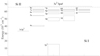 |
Fig. 1 Partial energy level diagram of Si I. The energy level values are from Martin & Zalubas (1983). Each box consists of several levels. |
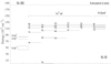 |
Fig. 2 Partial energy level diagram of Si II. The energy level values are from Martin & Zalubas (1983). Each box consists of several levels. |
3 Theoretical method
We used the RMCDHF method (Jönsson et al. 2013,2017) to calculate the oscillator strengths of Si I and Si II transitions. In this method, atomic state functions (ASF) are represented by linear combinations of configuration state functions (CSFs):
 (5)
(5)
In the equation, γj represents the information of the CSFs, that is, parity, orbital occupancy, and angular coupling scheme. The terms J and MJ represent the angular quantum numbers, whereas P represents the parity, and finally cj indicates the mixing coefficients. The CSFs are built from one-electron Dirac orbitals in the form of
 (6)
(6)
where Pnκ(r) and Qnκ(r) are the large and small components of the radial wavefunction and X±κ,m(θ, φ) are two-component spin-orbit functions. In the relativistic self-consistent field procedure, we optimise both the radial parts of the Dirac orbitals and the expansion coefficients.
The calculations for Si I were made for target states belonging to the configurations shown in Table 1. These configurations are referred to as the multireference (MR). For the initial calculation, the ASFs include all CSFs that can be formed from the configurations in the MR. To improve the ASFs, we performed calculations with systematically enlarged CSF expansions. For Si I, after analysing the eigenvector compositions, we found that the replacement of 3s2 with 3p2 gives important configurations. In addition, the first correlating d orbital, the 3d′ orbital, overlaps with the 3s and 3p orbitals. Therefore, replacement of 3s with 3d′ gives additional significant configurations. In both cases, the substitutions give rise to CSFs with expansion coefficients in the range 0.1–0.25. For these reasons, we expanded the MR as shown in Table 2 and allowed CSF expansions to form from these configurations by restricted single and double orbital replacements with orbitals in an active set. We applied the restriction that 1s2 should be a closed shell and at most one replacement from 2s22p6. Froese Fischer (2005) performed detailed correlation studies for Si I and showed that including core-valence correlation removes the discrepancy between computed and experimental fine-structure splittings of 3s3p3 levels. For this reason, we included both the valence-valence correlation (i.e. replacements from the valence orbitals outside the 2s22p6 core) and the core-valence correlation (i.e. one replacement from the valence and one from 2s22p6). No replacements were allowed from 1s2, which is always closed. The orbitals in the active set were systematically extended to include the 13s, 12p, 12d, 11f, 10g, 9h, and 7i orbitals when accounting for the valence-valence correlation, and the number of CSFs was 8427 862. Additionally, to account for the core-valence correlation, we used an active set including the 10s, 9p, 7d, 6f, and 5g orbitals. The number of CSFs thus increased to 17 886 964.
For Si II, we kept the MR as given in Table 1 and allowed single and double replacements from the given configurations with the same restrictions as applied to Si I. At most, one replacement from 2s22p6 and 1s2 should be a closed shell. To account for the valence-valence correlation, we extended the orbitals in the active set to include the 13s, 12p, 12d, 12f, 11g, 9h, and 7i orbitals containing 1693 014 CSFs. The number of CSFs expands to 11 850 176 when the core-valence correlation is accounted for. In our calculations, we included the Breit-interaction and leading QED effects.
After determining the ASFs, we calculated the oscillator strengths as expectation values of the transition operator. The calculations were performed both in the length and velocity gauges (Grant 1974). As an indicator of accuracy, the oscillator strengths calculated with these two gauges should give the same value. We determined the uncertainty indicator as a relative difference between the two gauges, u(f)/f = (Al − Av)/max(Al, Av) (Ekman et al. 2014). In our calculations, the uncertainty indicator is very low for the transitions involving the low-lying states. However, the agreement between the length and velocity forms is slightly worse for transition from highly excited states, as discussed in Pehlivan Rhodin et al. (2017). In addition, we estimated the uncertainty of the lifetimes, which were used for deriving the log(𝑔f) values, from error propagation. Since the lifetime of an upper level is τu = 1/ΣiAi, the uncertainty contribution from each A value is weighted by its own BF, following the expression from error propagation.
Configurations of targeted states for Si I and Si II.
Extended multireference for Si I calculations.
4 Results and conclusions
4.1 Si I
One of the quality indicators of calculations is the ability to reproduce the energy structure. Table B.1 shows the good quality of our calculated energy levels when compared to the experimental energy values in NIST (Kramida et al. 2022), which are the values of Martin & Zalubas (1983). In addition, we included the energy values determined from other theoretical studies (Froese Fischer et al. 2006; Wu et al. 2016; Savukov 2016). In general, our calculations are in better agreement with the experimental values of Martin & Zalubas (1983) compared to previous calculations. Relative differences are as low as 0.2%. The Froese Fischer et al. (2006) values have the same relative differences; however, the calculations were only performed for the low-lying levels up to 3s23p3d 3Do.
In Table B.2, we compare our theoretical lifetimes with the lifetimes of Froese Fischer (2005) calculated with the Breit-Pauli approximation and with the experimental lifetimes of O’Brian & Lawler (1991) from laser-induced fluorescence. The uncertainties of our theoretical lifetimes are in the range of 5 to 10%. Overall, there is a very good agreement between our values and the values of Froese Fischer (2005), with an exception of shorter lifetimes for the 3p3d 3Fo levels and longer lifetimes for the 3p3d1 Po and 3Do levels in our calculations compared to the values in Froese Fischer (2005). When comparing these lifetimes with the experimental values of O’Brian & Lawler (1991), we found an improvement in the theoretical lifetimes with our calculation. The agreement between our values and those of O’Brian & Lawler (1991) is mostly within 2σ when using their experimental uncertainty, but there is a more than 20% variation for the high-lying 3p5d 1Po, 1Fo, 3Do, 3p7s1/2(1/2,1/2), 3p7s1/2(3/2,1/2), and 3p6d 1Fo levels. Figures A.1 and A.2 show these comparisons between our lifetime values and those of O’Brian & Lawler (1991) and Froese Fischer (2005). In Fig. A.1, the error bars include only the uncertainty from the experiments and no uncertainty added to the calculated values. The blue dotted line shows the 10% relative difference. From these figures, it can be seen that the agreement with the literature values is mostly within 10%. This is in agreement with the overall uncertainties of our calculated lifetimes.
We derived 17 log(𝑔ƒ) values from calculated lifetimes and experimental BFs for the infrared lines from the 3p4p 3D1,2, 3P1,2, and 3S1 levels with uncertainties in the ƒ-value varying from 3 to 10%, and 20% for two lines. We note that for strong lines, the uncertainty of the BF becomes negligible, and the uncertainty in the log 𝑔ƒ is determined by the uncertainty in the lifetime. (See the discussion by Sikström et al. (2002) for details.)
This is the first time that the log(𝑔ƒ) values of these lines have been determined from experimental BFs. To our knowledge, there are no lifetime measurements of these levels. The calculated lifetimes are dominated by the strong transition probabilities, and they can be computed accurately. For this reason, we combined our experimental BFs with our computed lifetime values. Additionally, we performed theoretical calculations and determined log(𝑔ƒ) values of transitions from levels up to 3p7s. We note that the transitions from states belonging to configurations including any of the 7p, 6f, 8s, 6d, and 5g orbitals are not included in the transition data table, as the differences in the velocity and length forms of the A values are large, on the order of 50%, for these transitions. Nevertheless, those orbitals were needed for accurate calculation of other orbitals with large radii, which is similar to the findings reported for the calculations of neutral magnesium in Pehlivan Rhodin et al. (2017). We scaled our calculated transition probabilities and log(𝑔ƒ) values to experimental wavelengths.
Figure A.3 shows a comparison of our experimental log(𝑔ƒ) values with our theoretical log(𝑔ƒ) values. The very good agreement between the two methods validates the quality of our theoretical values. Table B.3 presents our experimental log(𝑔ƒ) values with their uncertainties, corresponding theoretical log(𝑔ƒ) values with their uncertainties, the branching fractions, BFs, and the transition probabilities, Aul. We determined the uncertainties of the theoretical log(𝑔ƒ) values using the equations presented by Froese Fischer (2009). However, the difference between the observed and calculated transition energy is small compared to the difference in length and velocity gauges. Therefore, it is adequate to consider the relative difference between the two gauges as an uncertainty indicator, as suggested by Ekman et al. (2014) in Eq. (5).
In Fig. A.4, we compare our theoretical log(𝑔ƒ) values with the values of Froese Fischer et al. (2006). The calculations performed by Froese Fischer et al. (2006) were only for the lowest lying levels up to the 3p3d 3Do levels, whereas in our calculations we have included additional levels up to 3p7s1/2(3/2,1/2). There is a good agreement between our theoretical values and those of Froese Fischer et al. (2006). This further illustrates the quality of our calculation. Our values complement those of Froese Fischer et al. (2006) by covering many more levels.
In addition, we compared our theoretical log(𝑔ƒ) values with the experimental values of O’Brian & Lawler (1991). Figure A.5 shows the good agreement between these values. We note that the log(𝑔ƒ) = −2.47 value for the  transition and log(𝑔ƒ) = −3.17 value for the
  transition in O’Brian & Lawler (1991) are given as upper limits and differ from our theoretical values.
Moreover, we compared the differences between our experimental log(𝑔ƒ) values and scaled theoretical log(𝑔ƒ) as a function of the line strength, S, in Fig. A.6. In this way, we could eliminate the wavelength dependence of the log(𝑔ƒ) values and clearly see that the variation is larger for weak lines (small line strength values), as expected. We note that in this figure, we only added the uncertainty from the experimental log(𝑔ƒ) values. We made similar comparisons in Figs. A.7 and A.8 with values of Froese Fischer et al. (2006) and O’Brian & Lawler (1991), respectively. The differences are larger for weaker lines (i.e. lines with smaller line strengths). In Fig. A.8, the largest differences are from the transitions mentioned above ( and
and  ), where only the upper limits are given in O’Brian & Lawler (1991). In this figure, we only added the uncertainty of the experimental values.
In Table B.4, we present our extended set of theoretical log(𝑔ƒ) values in addition to the comparisons we made in Table B.3. The log(𝑔ƒ) are given together with the transition probabilities and the estimated relative uncertainties, u(ƒ)/ƒ, for each transition. The wavenumber and wavelength values presented are from the NIST database, which are the values from Reader et al. (1980). For most of the transitions, the estimated relative uncertainties are less than 10%. However, for some transitions, the uncertainties are very large. This is mostly due to difficulties in calculating the transition rates of lines with upper and lower levels that differ by two or more electrons, such as  , or intercombination lines, such as
  . The former transition rates are identically zero at the lowest approximation of the wavefunction and are induced by correlation effects. Thus, they are highly challenging to compute. We note that the effects of them have been studied by Bogdanovich et al. (2007). In relativistic theory, the rates of intercombination transitions are formed by large and cancelling contributions and are therefore difficult to calculate (Ynnerman & Froese Fischer 1995). Nevertheless, these transitions are included in the table, but we urge the reader to be aware of the uncertainties of the transitions they are interested in.
4.2 Si II
In Table B.5, we compare our calculated energy levels with the experimental values of Martin & Zalubas (1983) and the calculated values of Froese Fischer et al. (2006) and Aggarwal & Keenan (2014). On average, our values and those of Froese Fischer et al. (2006) agree very well with the experimental values. The relative differences with respect to the experimental values are as low as 0.2 and 0.4% on average, respectively. On the other hand, the relative differences of the Aggarwal & Keenan (2014) values are as high as 5% on average. This is an order of magnitude larger than for our calculations.
Table B.6 presents the theoretical lifetimes of this study together with the theoretical lifetimes of Froese Fischer et al. (2006) and the experimental values of Bashkin et al. (1980); Calamai et al. (1993); Bergeson & Lawler (1993), when available. Our theoretical data, with estimated uncertainties of 5% to 10%, agree with experiments within the combined uncertainties. In addition, most our values are in agreement with those of Froese Fischer et al. (2006), except for those from the lowest levels. Nevertheless, our values for those levels show much better agreement with experiments than the values of Froese Fischer et al. (2006) do. Comparisons between our values and those in the literature are shown in Figs. A.9 and A.10. We note that there are few values that have the same relative difference between our values and those of Froese Fischer et al. (2006), and they are close in energy levels; therefore, it is difficult to visually distinguish them in the plot.
In Fig. A.11, we compare our scaled log(𝑔ƒ) values with those of Froese Fischer et al. (2006). Froese Fischer et al. (2006) calculated the log(𝑔ƒ) values for transitions up to the 3s3p2 2P3/2 level, while our calculation included the  level. There is a good agreement between the values for the common transitions, and our additional data are complementary to those of Froese Fischer et al. (2006).
A comparison of our scaled log(𝑔ƒ) values with the recommended Bautista et al. (2009) values is presented in Fig. A.12. Bautista et al. (2009) calculated the log(𝑔ƒ) values for the levels of 3s23p, 3s3p2, 3s24s, and 3s33d configurations. The authors performed calculations using different codes and approximations, including relativistic Hartree-Fock (HFR), Breit-Pauli calculations based on the Thomas-Fermi-Dirac-Amaldi central potential, and Multiconfiguration Dirac Fock (MCDF), and they reported the recommended log(𝑔ƒ) values derived from the comparisons of these calculations and experiments in the literature. Our values agree with the recommended values of Bautista et al. (2009) within the uncertainties. The comparison of our theoretical results with the experimental values of Matheron et al. (2001) in Fig. A.13 shows a good agreement, except for the weakest line at λ4072.7 Å.
Moreover, we compared the log(𝑔ƒ) values as a function of the line strength, S. These comparisons are presented in Figs. A.14, A.15, and A.16. In the figures, our values are compared to those of Froese Fischer et al. (2006), Bautista et al. (2009), and Matheron et al. (2001), respectively. We note that we only added the uncertainties of the recommended values and experimental values. As the figures clearly show, the variation is larger for the weaker lines.
Laha et al. (2016b) suggested that the long-standing discrepancy between the theory and observations in the line intensity ratios of the Si II UV lines may be due to the atomic data. They did an analysis using the theoretical transition probabilities of Aggarwal & Keenan (2014). However, there are large variations between the Aggarwal & Keenan (2014) values and the previous theoretical values of Nahar (1998) as well as the experimental values of Calamai et al. (1993). Table B.7 presents the transitions Laha et al. (2016b) used together with the transition probabilities of our theoretical study, the experimental values of Calamai et al. (1993), and the theoretical values of Nahar (1998) and Aggarwal & Keenan (2014). We note that the uncertainties given in Calamai et al. (1993) are relative, while in Table B.7 we cite the absolute uncertainties. For the intercombination lines, it is clear that our values agree both with the experimental values and the theoretical ones of Nahar (1998) rather than those of Aggarwal & Keenan (2014). Moreover, our values for the 3s23p 2P ‐ 3s3p2 2D transitions are closer to Nahar (1998) values than to Aggarwal & Keenan (2014). Our new calculations and their agreement with the recommended values by Nahar (1998) indicate that the silicon disaster could be caused by insufficient plasma models instead of inaccurate atomic data.
Finally, Table B.8 presents the theoretical log(𝑔ƒ) values of this work together with the transition probabilities and the estimated relative uncertainties, u(f)/f, for each transition. The wavenumber and wavelength values are from the NIST database, which adopted the values in Reader et al. (1980). In general, the relative uncertainties are less than 10%, but for the two-electron transitions or intercombination lines, the relative uncertainties get larger.
5 Summary
In this article, we provide an extensive set of accurate experimental and theoretical log(𝑔ƒ) values. For the first time, we derived 17 log(𝑔ƒ) values of Si I lines in the infrared from experimental measurements, and we report data for 1500 Si I lines and 500 Si II lines. The experimental uncertainties of our f-values vary between 5% for the strong lines and 25% for the weak lines. The theoretical log(𝑔ƒ) values for the Si I lines in the range 161 nm to 6340 nm agree very well with the experimental values of this study and complete the missing transitions involving levels up to 3s23p7s (61970 cm−1). In addition, we provide accurate calculated log(𝑔ƒ) values of Si II lines from the levels up to 3s27f (122 483 cm−1) in the range 81 nm to 7324 nm.
Acknowledgements
We acknowledge the grants no 2011-4206, 2015-0947 and 2016-04185 from the Swedish Research Council (VR) and Crafoord foundation. The infrared FTS at the Edlén laboratory is made available through a grant from the Knut and Alice Wallenberg Foundation. We acknowledge a project grant from the Krapperup Foundation no 2017-0123. We are grateful for valuable comments from an anonymous referees on the current and earlier version of this manuscript.
Appendix A Figures
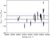 |
Fig. A.1 Relative difference of the Si I lifetimes between this work and the experimental values of O’Brian & Lawler (1991). The blue dashed line indicates a 10% difference. The error bars show the uncertainties of O’Brian & Lawler (1991). |
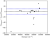 |
Fig. A.2 Relative difference of the Si I lifetimes between this work and the calculated values of Froese Fischer (2005). The blue dashed line indicates a 10% difference. |
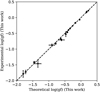 |
Fig. A.3 Comparison between the Si I log(𝑔f) values of this study determined from the experiments and scaled theoretical calculations. |
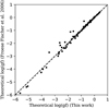 |
Fig. A.4 Comparison between the Si I scaled theoretical log(𝑔f) values of this study and those of Froese Fischer et al. (2006). |
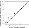 |
Fig. A.5 Comparison between the Si I scaled theoretical log(𝑔f) values of this study and the experimental values of O’ Brian & Lawler (1991). |
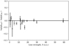 |
Fig. A.6 Difference between the Si I log(𝑔f) values of this study determined from the experiments and scaled theoretical calculations and their variation with the line strength, S. The errors bars shown are the experimental uncertainties. |
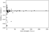 |
Fig. A.7 Difference between the Si II log(𝑔f) values of this study determined from the scaled theoretical calculations and those of Froese Fischer et al. (2006) and their variation with the line strength, S. |
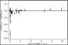 |
Fig. A.8 Difference between the Si I log(𝑔f) values of this study determined from the scaled theoretical calculations and the experimental values of O’Brian & Lawler (1991) and their variation with the line strength, S. The error bars shown are from O’Brian & Lawler (1991). |
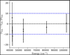 |
Fig. A.9 Relative difference of the Si II lifetimes between this work and the experimental values of Bashkin et al. (1980); Calamai et al. (1993); Bergeson & Lawler (1993), as reported in Table B.6. The blue dotted line indicates a 10% difference. |
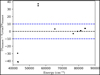 |
Fig. A.10 Relative difference of the Si II lifetimes between this work and the calculated values of Froese Fischer et al. (2006). The blue dotted line indicates a 10% difference. |
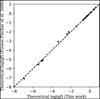 |
Fig. A.11 Comparison between the Si II theoretical log(𝑔f) values of this study and those of Froese Fischer et al. (2006). |
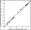 |
Fig. A.12 Comparison between the Si II theoretical log(𝑔f) values of this study and the values recommended by Bautista et al. (2009). |
 |
Fig. A.13 Comparison between the Si II theoretical log(𝑔f) values of this study and the experimental values of Matheron et al. (2001). |
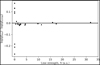 |
Fig. A.14 Difference between the Si II log(𝑔f) values of this study determined from the scaled theoretical calculations and those of Froese Fischer et al. (2006) and their variation with the line strength, S. |
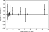 |
Fig. A.15 Difference between the Si II log(𝑔f) values of this study determined from the scaled theoretical calculations and the recommended values of Bautista et al. (2009) and their variation with the line strength, S. |
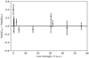 |
Fig. A.16 Difference between the Si II log(𝑔f) values of this study determined from the scaled theoretical calculations and the experimental values of Matheron et al. (2001) and their variation with the line strength, S. |
Appendix B Tables
Comparison of the Si I energy levels calculated in this work with the experimental values of Martin & Zalubas (1983) and other calculated values from Wu et al. (2016); Froese Fischer et al. (2006); Savukov (2015). Energies presented are in inverse centimeters (cm−1). This table is available in its entirety at the CDS.
Presentation of the radiative lifetimes of Si I levels computed in this work, τthis calc., and comparison with the theoretical values of Froese Fischer (2005) and the experimental values of O’Brian & Lawler (1991), when possible. Excitation energies are from Martin & Zalubas (1983). The uncertainties of the lifetimes vary, see text for details. This table is available in its entirety at the CDS.
Presentation of log(𝑔f) values for Si I based on the experimental branching fractions and the theoretical lifetimes of this work together with the wavelength, λ; wavenumber, σ; branching fraction, BF; transition probability, A; and corresponding theoretical log(𝑔f) values of this work.
Presentation of the computed Si I radiative transition data together with the relative uncertainties in f-values. An explanation of the columns is given at the end of the table. The table is published at CDS in electronic form, where it is available in its entirety.
Comparison of the Si II energy levels calculated in this work with the experimental values of Martin & Zalubas (1983) and calculated values from Froese Fischer et al. (2006); Aggarwal & Keenan (2014). Energies presented are in inverse centimeters (cm-1). This table is available in its entirety at the CDS.
Presentation of the radiative lifetimes (in nanoseconds) of Si II levels computed in this work, τthis calc., and comparison with other computed values and experimental values. Excitation energies are from Martin & Zalubas (1983). Energies presented are in inverse centimeters (cm−1). This table is available in its entirety at the CDS.
Comparison of Sill A values from this study with the existing experimental and theoretical values.
Presentation of the computed radiative transition data of Si II lines together with the relative uncertainties in f-values. An explanation of the columns is given at the end of the table. The table is published at CDS in electronic form.
References
- Aggarwal, K. M., & Keenan, F. P. 2014, MNRAS, 442, 388 [NASA ADS] [CrossRef] [Google Scholar]
- Amarsi, A. M., & Asplund, M. 2017, MNRAS, 464, 264 [Google Scholar]
- Asplund, M. 2000, A&A, 359, 755 [NASA ADS] [Google Scholar]
- Asplund, M., Grevesse, N., Sauval, A. J., & Scott, P. 2009, ARA&A, 47, 481 [NASA ADS] [CrossRef] [Google Scholar]
- Asplund, M., Amarsi, A. M., & Grevesse, N. 2021, A&A, 653, A141 [NASA ADS] [CrossRef] [EDP Sciences] [Google Scholar]
- Baldwin, J. A., Ferland, G. J., Korista, K. T., et al. 1996, ApJ, 461, 664 [NASA ADS] [CrossRef] [Google Scholar]
- Bashkin, S., Astner, G., Mannervik, S., et al. 1980, Phys. Scr, 21, 820 [Google Scholar]
- Bautista, M. A., Quinet, P., Palmeri, P., et al. 2009, A&A, 508, 1527 [NASA ADS] [CrossRef] [EDP Sciences] [Google Scholar]
- Becker, U., Kerkhoff, H., Kwiatkowski, M., et al. 1980a, Phys. Lett. A, 76, 125 [NASA ADS] [CrossRef] [Google Scholar]
- Becker, U., Zimmermann, P., & Holweger, H. 1980b, Geochim. Cosmochim. Acta, 44, 2145 [NASA ADS] [CrossRef] [Google Scholar]
- Bensby, T., Feltzing, S., & Oey, M. S. 2014, A&A, 562, A71 [NASA ADS] [CrossRef] [EDP Sciences] [Google Scholar]
- Bergemann, M., Kudritzki, R.-P., Würl, M., et al. 2013, ApJ, 764, 115 [NASA ADS] [CrossRef] [Google Scholar]
- Bergeson, S. D., & Lawler, J. E. 1993, ApJ, 414, L137 [NASA ADS] [CrossRef] [Google Scholar]
- Blanco, F., Botho, B., & Campos, J. 1995, Phys. Scr, 52, 628 [Google Scholar]
- Bogdanovich, P., Karpuskiene, R., & Rancova, O. 2007, Phys. Scr, 75, 669 [Google Scholar]
- Brewer, J. M., Fischer, D. A., Valenti, J. A., & Piskunov, N. 2016, ApJS, 225, 32 [Google Scholar]
- Buder, S., Sharma, S., Kos, J., et al. 2021, MNRAS, 506, 150 [NASA ADS] [CrossRef] [Google Scholar]
- Burheim, M., Hartman, H., & Nilsson, H. 2023, A&A, 672, A197 [NASA ADS] [CrossRef] [EDP Sciences] [Google Scholar]
- Calamai, A. G., Smith, P. L., & Bergeson, S. D. 1993, ApJ, 415, L59 [NASA ADS] [CrossRef] [Google Scholar]
- Cashman, F. H., Kulkarni, V. P., Kisielius, R., Ferland, G. J., & Bogdanovich, P. 2017, ApJS, 230, 8 [NASA ADS] [CrossRef] [Google Scholar]
- Charro, E., & Martín, I. 2000, ApJS, 126, 551 [NASA ADS] [CrossRef] [Google Scholar]
- Coutinho, L. H., & Trigueiros, A. G. 2002, J. Quant. Spectrosc. Radiat. Transf., 75, 357 [NASA ADS] [CrossRef] [Google Scholar]
- Dufton, P. L., Keenan, F. P., Hibbert, A., et al. 1991, MNRAS, 253, 474 [NASA ADS] [CrossRef] [Google Scholar]
- Ekman, J., Godefroid, M., & Hartman, H. 2014, Atoms, 2, 215 [CrossRef] [Google Scholar]
- Engström, L. 1998, GFit, A Computer Program to Determine Peak Positions and Intensities in Experimental Spectra., Technical Report LRAP-232, Atomic Physics, Lund University [Google Scholar]
- Engström, L. 2014, GFit, https://www.atomic.physics.lu.se/fileadmin/atomfysik/AF_Personal/Professors/GFit.html [Google Scholar]
- Froese Fischer, C. 2005, Phys. Rev. A, 71, 042506 [Google Scholar]
- Froese Fischer, C. 2009, Phys. Scrip. Vol. T, 134, 014019 [Google Scholar]
- Froese Fischer, C., Tachiev, G., & Irimia, A. 2006, Atm. Data Nucl. Data Tables, 92, 607 [NASA ADS] [CrossRef] [Google Scholar]
- Garz, T. 1973, A&A, 26, 471 [NASA ADS] [Google Scholar]
- Grant, I. P. 1974, J. Phys. B Atm. Mol. Phys., 7, 1458 [NASA ADS] [CrossRef] [Google Scholar]
- Hanke, M., Hansen, C. J., Ludwig, H.-G., et al. 2020, A&A, 635, A104 [NASA ADS] [CrossRef] [EDP Sciences] [Google Scholar]
- Heiter, U., Lind, K., Bergemann, M., et al. 2021, A&A, 645, A106 [EDP Sciences] [Google Scholar]
- Howes, L. M., Asplund, M., Keller, S. C., et al. 2016, MNRAS, 460, 884 [NASA ADS] [CrossRef] [Google Scholar]
- Jofré, E., Petrucci, R., Saffe, C., et al. 2015, A&A, 574, A50 [Google Scholar]
- Jönsson, H., Ryde, N., Nissen, P. E., et al. 2011, A&A, 530, A144 [NASA ADS] [CrossRef] [EDP Sciences] [Google Scholar]
- Jönsson, P., Gaigalas, G., Bieroń, J., Fischer, C. F., & Grant, I. P. 2013, Comp. Phys. Commun., 184, 2197 [CrossRef] [Google Scholar]
- Jönsson, P., Gaigalas, G., Rynkun, P., et al. 2017, Atoms, 5, 16 [CrossRef] [Google Scholar]
- Judge, P. G., Carpenter, K. G., & Harper, G. M. 1991, MNRAS, 253, 123 [NASA ADS] [CrossRef] [Google Scholar]
- Kramida, A., Ralchenko, Yu., Reader, J., & NIST ASD Team 2022, NIST Atomic Spectra Database (ver. 5.10), [Online]. Available: https://physics.nist.gov/asd. National Institute of Standards and Technology, Gaithersburg, MD [Google Scholar]
- Kurucz, R. M. 2016, Kurucz database, http://kurucz.harvard.edu/atoms/1400/ [Google Scholar]
- Laha, S., Keenan, F. P., Ferland, G. J., Ramsbottom, C. A., & Aggarwal, K. M. 2016a, ApJ, 825, 28 [NASA ADS] [CrossRef] [Google Scholar]
- Laha, S., Keenan, F. P., Ferland, G. J., et al. 2016b, MNRAS, 455, 3405 [NASA ADS] [CrossRef] [Google Scholar]
- Magg, E., Bergemann, M., Serenelli, A., et al. 2022, A&A, 661, A140 [NASA ADS] [CrossRef] [EDP Sciences] [Google Scholar]
- Martin, W. C., & Zalubas, R. 1983, J. Phys. Chem. Ref. Data, 12, 323 [NASA ADS] [CrossRef] [Google Scholar]
- Mashonkina, L. 2020, MNRAS, 493, 6095 [CrossRef] [Google Scholar]
- Matheron, P., Escarguel, A., Redon, R., Lesage, A., & Richou, J. 2001, J. Quant. Spectrosc. Radiat. Transf., 69, 535 [NASA ADS] [CrossRef] [Google Scholar]
- Mikolaitis, Š., Hill, V., Recio-Blanco, A., et al. 2014, A&A, 572, A33 [NASA ADS] [CrossRef] [EDP Sciences] [Google Scholar]
- Nahar, S. N. 1993, Phys. Scr, 48, 297 [Google Scholar]
- Nahar, S. N. 1998, Atm. Data Nucl. Data Tables, 68, 183 [NASA ADS] [CrossRef] [Google Scholar]
- O’Brian, T. R., & Lawler, J. E. 1991, Phys. Rev. A, 44, 7134 [CrossRef] [Google Scholar]
- Pehlivan, A., Nilsson, H., & Hartman, H. 2015, A&A, 582, A98 [NASA ADS] [CrossRef] [EDP Sciences] [Google Scholar]
- Pehlivan Rhodin, A., Hartman, H., Nilsson, H., & Jönsson, P. 2017, A&A, 598, A102 [NASA ADS] [CrossRef] [EDP Sciences] [Google Scholar]
- Radziemski, L. J., Jr., & Andrew, K. L. 1965, J. Opt. Soc. Am., 55, 474 [NASA ADS] [CrossRef] [Google Scholar]
- Reader, J., Corliss, C. H., Wiese, W. L., & Martin, G. A. 1980, Wavelengths and transition probabilities for atoms and atomic ions: Part 1. Wavelengths, part 2. Transition probabilities (U.S. Government Printing Office) [Google Scholar]
- Rosman, K. J. R., & Taylor, P. D. P. 1998, J. Phys. Chem. Ref. Data, 27, 1275 [Google Scholar]
- Savukov, I. M. 2015, Phys. Rev. A, 91, 022514 [Google Scholar]
- Savukov, I. M. 2016, Phys. Rev. A, 93, 022511 [Google Scholar]
- Scott, P., Grevesse, N., Asplund, M., et al. 2015, A&A, 573, A25 [NASA ADS] [CrossRef] [EDP Sciences] [Google Scholar]
- Shaltout, A. M. K., Beheary, M. M., Bakry, A., & Ichimoto, K. 2013, MNRAS, 430, 2979 [CrossRef] [Google Scholar]
- Shchukina, N. G., Sukhorukov, A. V., & Trujillo Bueno, J. 2017, A&A, 603, A98 [NASA ADS] [CrossRef] [EDP Sciences] [Google Scholar]
- Shi, J. R., Gehren, T., Butler, K., Mashonkina, L. I., & Zhao, G. 2008, A&A, 486, 303 [NASA ADS] [CrossRef] [EDP Sciences] [Google Scholar]
- Shi, J. R., Takada-Hidai, M., Takeda, Y., et al. 2012, ApJ, 755, 36 [NASA ADS] [CrossRef] [Google Scholar]
- Sikström, C. M., Nilsson, H., Litzen, U., Blom, A., & Lundberg, H. 2002, J. Quant. Spectrosc. Radiat. Transf., 74, 355 [CrossRef] [Google Scholar]
- Smith, P. L., Huber, M. C. E., Tozzi, G. P., et al. 1987, ApJ, 322, 573 [NASA ADS] [CrossRef] [Google Scholar]
- Smith, V. V., Bizyaev, D., Cunha, K., et al. 2021, AJ, 161, 254 [NASA ADS] [CrossRef] [Google Scholar]
- Tan, K., Shi, J., Takada-Hidai, M., Takeda, Y., & Zhao, G. 2016, ApJ, 823, 36 [NASA ADS] [CrossRef] [Google Scholar]
- Tayal, S. S. 2007, J. Phys. B Atm. Mol. Phys., 40, 2551 [NASA ADS] [CrossRef] [Google Scholar]
- Tsujimoto, T., Nomoto, K., Yoshii, Y., et al. 1995, MNRAS, 277, 945 [Google Scholar]
- Woosley, S. E., & Weaver, T. A. 1995, ApJS, 101, 181 [Google Scholar]
- Wu, M., Bian, G., Li, X., et al. 2016, Canadian J. Phys., 94, 359 [NASA ADS] [CrossRef] [Google Scholar]
- Ynnerman, A., & Froese Fischer, C. 1995, Phys. Rev. A, 51, 2020 [Google Scholar]
- Zhang, J., Shi, J., Pan, K., Allende Prieto, C., & Liu, C. 2016, ApJ, 833, 137 [NASA ADS] [CrossRef] [Google Scholar]
All Tables
Comparison of the Si I energy levels calculated in this work with the experimental values of Martin & Zalubas (1983) and other calculated values from Wu et al. (2016); Froese Fischer et al. (2006); Savukov (2015). Energies presented are in inverse centimeters (cm−1). This table is available in its entirety at the CDS.
Presentation of the radiative lifetimes of Si I levels computed in this work, τthis calc., and comparison with the theoretical values of Froese Fischer (2005) and the experimental values of O’Brian & Lawler (1991), when possible. Excitation energies are from Martin & Zalubas (1983). The uncertainties of the lifetimes vary, see text for details. This table is available in its entirety at the CDS.
Presentation of log(𝑔f) values for Si I based on the experimental branching fractions and the theoretical lifetimes of this work together with the wavelength, λ; wavenumber, σ; branching fraction, BF; transition probability, A; and corresponding theoretical log(𝑔f) values of this work.
Presentation of the computed Si I radiative transition data together with the relative uncertainties in f-values. An explanation of the columns is given at the end of the table. The table is published at CDS in electronic form, where it is available in its entirety.
Comparison of the Si II energy levels calculated in this work with the experimental values of Martin & Zalubas (1983) and calculated values from Froese Fischer et al. (2006); Aggarwal & Keenan (2014). Energies presented are in inverse centimeters (cm-1). This table is available in its entirety at the CDS.
Presentation of the radiative lifetimes (in nanoseconds) of Si II levels computed in this work, τthis calc., and comparison with other computed values and experimental values. Excitation energies are from Martin & Zalubas (1983). Energies presented are in inverse centimeters (cm−1). This table is available in its entirety at the CDS.
Comparison of Sill A values from this study with the existing experimental and theoretical values.
Presentation of the computed radiative transition data of Si II lines together with the relative uncertainties in f-values. An explanation of the columns is given at the end of the table. The table is published at CDS in electronic form.
All Figures
|
Fig. 1 Partial energy level diagram of Si I. The energy level values are from Martin & Zalubas (1983). Each box consists of several levels. |
| In the text | |
|
Fig. 2 Partial energy level diagram of Si II. The energy level values are from Martin & Zalubas (1983). Each box consists of several levels. |
| In the text | |
|
Fig. A.1 Relative difference of the Si I lifetimes between this work and the experimental values of O’Brian & Lawler (1991). The blue dashed line indicates a 10% difference. The error bars show the uncertainties of O’Brian & Lawler (1991). |
| In the text | |
|
Fig. A.2 Relative difference of the Si I lifetimes between this work and the calculated values of Froese Fischer (2005). The blue dashed line indicates a 10% difference. |
| In the text | |
|
Fig. A.3 Comparison between the Si I log(𝑔f) values of this study determined from the experiments and scaled theoretical calculations. |
| In the text | |
|
Fig. A.4 Comparison between the Si I scaled theoretical log(𝑔f) values of this study and those of Froese Fischer et al. (2006). |
| In the text | |
|
Fig. A.5 Comparison between the Si I scaled theoretical log(𝑔f) values of this study and the experimental values of O’ Brian & Lawler (1991). |
| In the text | |
|
Fig. A.6 Difference between the Si I log(𝑔f) values of this study determined from the experiments and scaled theoretical calculations and their variation with the line strength, S. The errors bars shown are the experimental uncertainties. |
| In the text | |
|
Fig. A.7 Difference between the Si II log(𝑔f) values of this study determined from the scaled theoretical calculations and those of Froese Fischer et al. (2006) and their variation with the line strength, S. |
| In the text | |
|
Fig. A.8 Difference between the Si I log(𝑔f) values of this study determined from the scaled theoretical calculations and the experimental values of O’Brian & Lawler (1991) and their variation with the line strength, S. The error bars shown are from O’Brian & Lawler (1991). |
| In the text | |
|
Fig. A.9 Relative difference of the Si II lifetimes between this work and the experimental values of Bashkin et al. (1980); Calamai et al. (1993); Bergeson & Lawler (1993), as reported in Table B.6. The blue dotted line indicates a 10% difference. |
| In the text | |
|
Fig. A.10 Relative difference of the Si II lifetimes between this work and the calculated values of Froese Fischer et al. (2006). The blue dotted line indicates a 10% difference. |
| In the text | |
|
Fig. A.11 Comparison between the Si II theoretical log(𝑔f) values of this study and those of Froese Fischer et al. (2006). |
| In the text | |
|
Fig. A.12 Comparison between the Si II theoretical log(𝑔f) values of this study and the values recommended by Bautista et al. (2009). |
| In the text | |
|
Fig. A.13 Comparison between the Si II theoretical log(𝑔f) values of this study and the experimental values of Matheron et al. (2001). |
| In the text | |
|
Fig. A.14 Difference between the Si II log(𝑔f) values of this study determined from the scaled theoretical calculations and those of Froese Fischer et al. (2006) and their variation with the line strength, S. |
| In the text | |
|
Fig. A.15 Difference between the Si II log(𝑔f) values of this study determined from the scaled theoretical calculations and the recommended values of Bautista et al. (2009) and their variation with the line strength, S. |
| In the text | |
|
Fig. A.16 Difference between the Si II log(𝑔f) values of this study determined from the scaled theoretical calculations and the experimental values of Matheron et al. (2001) and their variation with the line strength, S. |
| In the text | |
Current usage metrics show cumulative count of Article Views (full-text article views including HTML views, PDF and ePub downloads, according to the available data) and Abstracts Views on Vision4Press platform.
Data correspond to usage on the plateform after 2015. The current usage metrics is available 48-96 hours after online publication and is updated daily on week days.
Initial download of the metrics may take a while.