| Issue |
A&A
Volume 674, June 2023
|
|
|---|---|---|
| Article Number | A148 | |
| Number of page(s) | 8 | |
| Section | Galactic structure, stellar clusters and populations | |
| DOI | https://doi.org/10.1051/0004-6361/202245449 | |
| Published online | 16 June 2023 | |
Globular clusters in the Galactic center region: Expected behavior within the infall and merger scenario⋆
1
INAF – Osservatorio Astronomico di Roma, Via di Frascati 33, 00040 Monteporzio Catone, Italy
e-mail: maria.navarro@inaf.it
2
Dipartimento di Fisica, Università degli Studi di Roma “La Sapienza”, P.le Aldo Moro, 2, 00185 Rome, Italy
3
Department of Physics and Astronomy, University of Padova, Via Marzolo 8, 35131 Padova, Italy
4
Departamento de Ciencias Físicas, Facultad de Ciencias Exactas, Universidad Andrés Bello, Av. Fernández Concha 700, Las Condes, Santiago, Chile
5
Vatican Observatory, 00120 Vatican City State, Italy
6
Departamento de Fisica, Universidade Federal de Santa Catarina, Trinidade, 88040-900 Florianópolis, Brazil
Received:
12
November
2022
Accepted:
19
January
2023
In this work, we reexamine the infall and merger scenario of massive clusters in the Milky Way’s potential well as a plausible Milky Way formation mechanism. We aim to understand how the stars of the merging clusters are redistributed during and after the merger process. We used, for the first time, high-resolution simulations with concentrated in the 300 pc around the Galactic center. We adopted simulations developed in the framework of the Modelling the Evolution of Galactic Nuclei (MEGaN) project. We compared the evolution of representative clusters in the mass and concentration basis in the vicinity of a supermassive black hole. We used the spatial distribution, density profile, and the 50% Lagrange radius (half mass radius) as indicators along the complete simulation to study the evolutionary shape in physical and velocity space and the final fate of these representative clusters. We find that the least massive clusters are quickly (< 10 Myr) destroyed. On the other hand, the most massive clusters have a long evolution, showing variations in the morphology, especially after each passage close to the supermassive black hole. The deformation of the clusters depends on the concentration, with general deformations for the least concentrated clusters and outer strains for the more concentrated ones. At the end of the simulation, a dense concentration of stars belonging to the clusters was formed. The particles that belong to the most massive and most concentrated clusters are concentrated in the innermost regions, meaning that the most massive and concentrated clusters contribute a more significant fraction of particles to the final concentration. This finding suggests that the population of stars of the nuclear star cluster formed through this mechanism comes from massive clusters rather than low-mass globular clusters.
Key words: Galaxy: formation / Galaxy: evolution / Galaxy: center / globular clusters: general
Movies associated to Figs. 4 and 5 are available at https://www.aanda.org.
© The Authors 2023
 Open Access article, published by EDP Sciences, under the terms of the Creative Commons Attribution License (https://creativecommons.org/licenses/by/4.0), which permits unrestricted use, distribution, and reproduction in any medium, provided the original work is properly cited.
This article is published in open access under the Subscribe to Open model. Subscribe to A&A to support open access publication.
1. Introduction
Several mechanisms have been proposed within the framework of galactic formation. Among the most widely accepted scenarios, the monolithic collapse model is notable, given its support of galactic formation via the collapse of a massive gas cloud. This scenario was first proposed by Eggen et al. (1962) and it now known as the ELS model. Another proposed scenario is the hierarchical model, a generic feature of cold dark matter (CDM) models, which suggests that the galaxies were formed by building blocks that formed first and then, the Galaxy was formed from smaller galaxies carrying globular clusters (GCs) with them, and deposited them mainly in the outskirts of the Galactic halo (White & Rees 1978; Baugh et al. 1996; Neistein et al. 2006). Overall, GCs are the oldest stellar systems known and they provide information that is vital to improving our understanding the earliest stages of the Milky Way.
From an observational point of view, the census of GCs in the Milky Way increased in number in the last years, reaching 156 GCs (Harris 2010), with many more candidates to be confirmed (Minniti et al. 2017; Garro et al. 2022a,b). One of the most critical limitations of studying GCs is extinction, which prevents the detection of clusters in the densest areas, such as the innermost region of the Milky Way, where we expect to find them and also their remnants because the potential well of the Galaxy is deeper and the disruptive dynamical effects should be stronger. This situation is improved with the new era of infrared surveys such as 2MASS (Skrutskie et al. 2006) and VVV Survey (Minniti et al. 2010). Minniti et al. (2021) investigated the GCs in the innermost regions of the Milky Way. They confirmed that VVV-GC002 is the closest known GC to the Galactic center. This metal-rich GC located at only 1.1 deg from the Galactic center, equivalent to RG = 0.4 kpc, was discovered initially by Moni Bidin et al. (2011).
Minniti et al. (2021) also found that there appears to be a forbidden zone of radius RG ∼ 0.1 kpc around the Galactic center, where GCs are crushed, and only young clusters can be seen. These young clusters would presumably not last long (Habibi et al. 2013, 2014; Hosek et al. 2015; Rui et al. 2019; Libralato et al. 2020, 2022). The debris of destroyed GCs might be found in this zone of tidal disruption surrounding the supermassive black hole (BH). Some of these destroyed primordial GCs (hereafter PGCs) may have helped build the massive nuclear star cluster at the center of our Galaxy (Capuzzo-Dolcetta 1993; Arca-Sedda & Capuzzo-Dolcetta 2014). This scenario is also supported by the presence of RR Lyrae stars in this region (Minniti 1995; Navarro et al. 2021), which are excellent indicators for studying the spatial distribution and dynamics of the population that comes from these GCs.
On the theoretical side, there have been numerous GC simulations that consider the different dynamical processes that affect their evolution (Chandrasekhar 1942; Hénon 1961; Larson 1970; Aarseth et al. 1974; Tremaine et al. 1975; Fall & Rees 1977, 1985; Heggie 1979, 2014; Tremaine & Weinberg 1984; Chernoff & Weinberg 1990; Vesperini & Heggie 1997; Gnedin & Ostriker 1997; Aarseth 1999; Baumgardt et al. 2002; Baumgardt & Makino 2003; Gieles et al. 2006; Gnedin et al. 2014; Carlberg 2017, 2018; Khoperskov et al. 2018). In particular, we are interested in the evolutionary shape in physical and velocity space and their survival and destruction mechanisms in the presence of a single supermassive BH, such as the one located at the center of the Milky Way. This study is crucial for its subsequent comparison with the population of clusters around the Galactic center, which has been increasing in recent years thanks to the new generation of infrared telescopes, which will further increase thanks to new missions such as the James Webb Space Telescope (JWST) and the Roman Space Telescope (WFIRST; Green et al. 2012; Spergel et al. 2015).
This paper presents new simulations for GCs in the Galactic center region. In Sect. 2, the details of the model and the initial conditions used are presented. Section 3 presents the method to study the evolution and morphology of the representative GCs in the vicinity of the supermassive BH. Our results are discussed in Sect. 4, and in Sect. 5, our findings are compared with the observations. Finally, our conclusions are presented in Sect. 5.
2. Galactic model and initial conditions
We used the HiGPUs code (Capuzzo-Dolcetta et al. 2013), an N-body code suitable for studying the dynamical evolution of stellar systems composed of up to 10 million stars with precision guaranteed by direct summation of the pair-wise forces. The code is written by combining C and C++ programming languages, and it is parallelized using a message passing interface (MPI), along with OpenMP and OpenCL to allow for the utilization of GPUs of different vendors. The code implements the Hermite’s sixth order time integration scheme (Nitadori & Makino 2008) with block time steps, allowing for high levels of precision and speed in studying the dynamical evolution of star systems. The coarse-grained parallelization establishes a one-to-one correspondence between MPI process and computational nodes, and each MPI process manages all the GPUs available per node.
For this analysis, we used simulations of GCs decaying to the center of the Galaxy (Arca-Sedda & Capuzzo-Dolcetta 2017, 2019). The simulation is performed in the framework of the Modelling the Evolution of Galactic Nuclei (MEGaN) project and consists of studying the evolution and merger of 41 GCs in the presence of a supermassive BH. We used a Dehnen model (Dehnen 1993) to model the Galactic bulge. The number of GCs is an arbitrary choice based on the limiting computing facilities.
The total number of particles is N = 220 = 1 048 576, which includes the Supermassive BH of MSMBH = 4.5 × 10⁶ M⊙, N = 478 107 particles belonging to the 41 GCs with stellar masses of M = 92 M⊙ and N = 570 468 background particles with particle masses of M = 180 M⊙ each. Due to computational limitations, the field particles are twice as massive as the cluster particles. The GCs have different density distributions and cover a range from N = 1477 to N = 21 383 particles, that is, from MGC = 105 M⊙ to MGC = 2 × 10⁶ M⊙ and core radii from Rc = 0.2 pc to Rc = 1.7 pc, which is the radius where the density has dropped to half the central value. Table 1 presents the main characteristics (core radius, number of particles, and total mass) of the GCs used in this simulation. The system’s total mass is M = 1.5 × 10⁸ M⊙ and the whole sample is initially confined within a radius of 300 pc, which is justified by previous effects of dynamical friction.
Properties of the Globular clusters in the simulation.
The simulation evolves during ∼200 Myr with timestamps of ΔT = 0.083125 Myr within a radius of 300 pc (∼2.1 deg). No external potential is applied in this simulation because the nuclear bulge is modeled in a self-consistent way with field stars. Further details of the simulations are presented in detail in our following article (Capuzzo-Dolcetta et al., in prep.).
Our first and foremost assumption is that the supermassive BH was already in place when these PGCs merged. The outcome of the simulations is that all of these PGCs no longer exist, having formed the nuclear star cluster. Figure 1 shows the 3D spatial distribution of the first snapshot of the simulation, where the 41 GCs begin to fall in the potential well of the Galaxy generated by background particles (which are not included in the figure). The blue dot represents the supermassive BH at the center of the Galaxy.
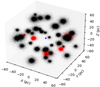 |
Fig. 1. First snapshot of the simulation plotted on a 60 pc scale, including the 41 Globular clusters with a wide range of masses. The blue dot corresponds to the supermassive BH in the center. The red clusters correspond to the clusters analyzed in this article selected according to mass and density, which act as representative samples for the analysis. |
We assume that star cluster positions and velocities follow the same distribution as the stars in the host galaxy. Thus, their initial conditions are drawn accordingly to the galaxy distribution function of the energy, which in our case, corresponds to the aforementioned Dehnen model. This choice is not unique and it is intrinsically linked to the star cluster formation process and its dependence on the galaxy’s structure and evolution. Still, it represents a good balance between the reliability of the initial conditions and the computational cost of the simulation. A different distribution of the cluster’s initial conditions would likely affect their overall evolution. For example, a more concentrated distribution of star clusters would favor a more significant amount of mass that is delivered into the Galactic center and likely a larger nuclear cluster mass. In contrast, a looser distribution would favor the tidal disruption of the clusters and the formation of a less massive and dense nuclear cluster (Arca-Sedda et al. 2015).
3. Method
We studied the evolution throughout the simulation of five representative clusters of different masses and concentrations. For the mass, we selected de clusters using the number of particles since the particle mass is constant (M = 92 M⊙). For the concentration, we used the concentration parameter (c) defined as c = log(rt/rc) where rt is the tidal radius, that is, the value of the radius at which the density profile reaches zero and rc the core radius which is the radius where the density has dropped to half the central value (King 1962).
The final sample consists of GC3 as the least massive, GC31 as the intermediate-mass, and GC23 as the most massive clusters. For the different concentrations, the clusters selected are GC3, GC26, and GC4 for the least, intermediate, and most concentrated, respectively. We note that GC3 was used in both analyses as the least massive and concentrated cluster. The five GCs selected are well distributed around the center (Fig. 1), which avoids any dependence on the initial position of the cluster that can influence the results. Table 2 lists the five clusters selected along with the number of particles (N), total mass (MGCs), Lagrange radius (rL), Tidal radius (rt), Core radius (rc), and concentration parameter (c).
Properties of the Globular clusters in the simulation according to mass (GC3, GC31, and GC23) and concentration (GC3, GC26, and GC4).
Figure 2 (mass comparison of GC3, GC31 and GC23) and Fig. 3 (concentration comparison of GC3, GC26, and GC4) present the spatial distribution of the clusters in the first snapshot, volumetric density profile, and Lagrange radius evolution. The differences in mass and concentration of the clusters selected for the comparison are clear from the spatial distribution and the density profile (left and middle panels of Figs. 2 and 3). Although the GC23 (lower panel of Fig. 2) is the most massive cluster of the simulation, the cluster GC4 (lower panel of Fig. 3) is more concentrated, reaching a value of ∼1010 particles per deg3.
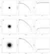 |
Fig. 2. Globular clusters with different masses. Left: spatial distribution of the particles belonging to the clusters in the first snapshot of the simulation. Middle: volumetric density profiles for the clusters in the first snapshots of the simulation. Right: implemented conversion from parsecs to degrees, assuming the Galactocentric distance R0 = 8.2 kpc (GRAVITY Collaboration 2019). Right: evolution of the 50% Lagrange radius of the clusters during the simulation. Top, middle, and lower panels show the least massive cluster (GC3), the intermediate mass cluster (GC31), and the most massive cluster (GC23), respectively. |
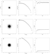 |
Fig. 3. Globular clusters with different concentrations. Left: spatial distribution of the particles belonging to the clusters in the first snapshot of the simulation. Middle: volumetric density profiles for the clusters in the first snapshots of the simulation. Right: implemented conversion from parsecs to degrees, assuming the Galactocentric distance R0 = 8.2 kpc. (GRAVITY Collaboration 2019). Right: evolution of the 50% Lagrange radius of the clusters during the simulation. Top, middle, and lower panels show the least massive cluster (GC3), the intermediate mass cluster (GC26), and the most massive cluster (GC4), respectively. |
In Fig. 4 (mass comparison of GC3, GC31 and GC23) and Fig. 5 (concentration comparison of GC3, GC26 and GC4) a graphical representation of the spatial distribution of three representative snapshots at t = 0 Myr, t = 8.3 Myr, and t = 41.5 Myr are shown. We show three representative snapshots, but the complete evolution was used to analyze the evolution in morphology properly. The full animations of the GCs evolution are available in online version of this paper.
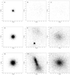 |
Fig. 4. Spatial distribution of the least massive cluster GC3 during the simulation, shown at the top. Middle: intermediate mass cluster GC31. Bottom: most massive cluster GC23. Left plots show the first snapshot of the simulation (t = 0 Myr), while the middle and right plots correspond to t = 8.3 Myr and t = 41.5 Myr, respectively. Complete animations for the simulations are available online. |
These simulations clearly show that effect of the supermassive BH is truly devastating. All GCs are destroyed (most of them very rapidly) and their debris mixed. These remains end up forming an extended structure around the supermassive BH that is akin to a nuclear star cluster. During the process, we observe the emergence of complex features in the individual GCs. When observed from different viewing angles, these features appear as threads, multiple blobs, shells, sausages, and so on. We also note that thin long, and coherent tidal tails, which are very common in disrupting halo GCs, are not present in these simulations.
4. Results
The evolution of the different clusters can be analyzed from different points of view, as discussed in the following. In terms of morphology and survival, we used two indicators to evaluate the evolution of the different clusters, the 50% Lagrange radius (half-mass radius), as shown in the right panels of Figs. 2 and 3, and the graphical representation of the spatial distribution of the clusters during the complete simulation. The latter is displayed as three representative snapshots in Figs. 4 and 5, whereas the full animations of the GCs evolution shown in these figures are available in the online version of this paper to illustrate the morphological changes.
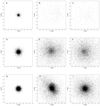 |
Fig. 5. Spatial distribution of the least concentrated cluster GC3 during the simulation, shown at the top. Middle: intermediate concentration cluster GC26. Bottom: most concentrated cluster GC4. Left plots show the first snapshot of the simulation (t = 0 Myr), while the middle and right plots correspond to t = 8.3 Myr and t = 41.5 Myr, respectively. Complete animations for the simulations are available online. |
When analyzing the GCs of different masses (Figs. 2 and 4), the results show that the least massive cluster (GC3) is completely destroyed and falls into the potential well very quickly. Panel B of Fig. 4 shows that the cluster is already completely disrupted at t = 8.3 Myr. This is also evident in the Lagrange radius evolution in panel C of Fig. 2, where the cluster experiences prominent variations in the initial snapshots, reaching a value of R = 0.511 deg (72.9 pc) at 8 Myr. The intermediate-mass cluster (GC31) keeps its high stellar concentration core during the first part of the simulation and then no longer has a defined shape. In panel E of Fig. 4, the core is still clearly defined at t = 8.3 Myr, but in panel F at t = 41.5 Myr, we can see that it is destroyed. The Lagrange radius of this cluster stabilizes at ∼19 Myr, without presenting significant variations in size, reaching a value of R = 0.234 deg (33.3 pc). The most massive cluster (GC23) instead undergoes deformations and elongations of the most central and concentrated part (see H panel of Fig. 4) and then it is destroyed, leaving an appreciable concentration of stars in the center. The Lagrange radius evolution shows a bump at ∼5 Myr following its first passage near the Galactic center, where the potential is maximized (I panel of Fig. 2). This means that the destructive effect of the supermassive BH is more critical than that of cluster-cluster collisions. Then this massive GC takes 25.7 Myr to reach stability at a value of R = 0.136 deg (19.4 pc).
On the other hand, the clusters of different concentrations exhibit different behavior (Figs. 3 and 5). The least concentrated cluster corresponds to the least massive already analyzed (GC3). As mentioned, this cluster is disrupted quickly, spreading its stars into the field. The intermediate concentration one (GC26) does not keep the core for a long time. According to panels D, E, and F of Fig. 5, at t = 8.3 Myr, the cluster no longer has a defined shape. The Lagrange radius begins to stabilize at 17 Myr but reaches stability at 36 Myr, with a value of R = 0.165 deg (23.5 pc) (see F panel of Fig. 3). In the lower panels (G, H, and I of Fig. 5), the most concentrated cluster (GC4) exhibits various changing shapes in its outskirts while the central core survives. It begins to stabilize at 30 Myr and reaches stability at 42 Myr with a Lagrange radius of only R = 0.065 deg (9.2 pc) (panel I of Fig. 3). Therefore, the least concentrated clusters are destroyed faster than the more concentrated ones at a given mass. The clusters’ morphological evolution and destruction during the simulation strongly depend on their mass and concentration.
At the end of the simulation, a concentrated nuclear star cluster is formed, containing the bulk of the total GC mass. Its evolution is discussed in detail by Navarro et al. (in prep.). We observe that for low mass and low concentration clusters (panel C of Figs. 2 and 3, respectively), the Lagrange radius stabilizes faster, reaching a higher value, meaning that the least massive and concentrated clusters disrupt fast and spread the particles around without yielding an evident concentration of stars around the Galactic center. The high mass and concentrated clusters (panel C of Figs. 2 and 3, respectively) reach smaller values for the Lagrange radius, meaning that the stars belonging to these clusters remain confined around the Galactic center after the simulation. This implies that the massive and concentrated GCs contribute to a higher percentage of stars in the Galactic center than the least massive GCs. Therefore, the population of stars concentrated in the Galactic center comes primarily from massive clusters.
It can also be observed that the massive clusters suffer deformations in their shapes (lower panels G, H, and I of Fig. 4). The deformation can be general or limited to the outer particles depending on the concentration of the cluster. We see that the morphology is directly affected by the passages of the clusters near the supermassive BH. Interestingly, a close passage by the central BH can split the cluster into two well-separated structures that are not necessarily symmetric as we find, for example, in GC tidal tails. This is shown as bumps in the Lagrange radius evolution at the moment when these passages occur. The clusters may exhibit different morphologies during this process.
Additionally, we studied the evolution of another sample of six clusters from the simulation, along with the parameters mentioned before. The test in terms of mass was also carried out for the clusters GC30, GC25, and GC14 as the second most massive, intermediate-mass, and least massive clusters. In terms of concentration, we also analyzed the clusters GC10, GC18, and GC11 as the second most concentrated, intermediate, and least concentrated clusters. The behavior is similar to the clusters selected here (GC3, GC4, GC23, GC26, and GC31) in terms of the morphology evolution and final distribution of particles depending on mass and concentration.
One of the motivations of our simulations has been to guide a future search for GCs hidden in the Galactic center region with the Roman Space Telescope. Still, this work implies that these GCs should be long gone within ∼300 pc. We thus chose to examine the specific example of VVV-GC002, the closest GCs to the Galactic center at RG = 400 pc (Minniti et al. 2021). Even though this distance range is just outside our simulations that reach 300 pc, we can predict that this GC should not have survived in that environment. Therefore, it either consists of the remains of a much more massive structure or it has formed farther away and is now observed close to the perigalactic of its orbit – or both assumptions may be true. The GCs of our simulation are massive and some are comparable in mass to VVV-GC002. However, a direct comparison with the orbital evolution of this cluster is not yet warranted because the orbit of VVV-GC002 is still unknown, as this GC lacks radial velocities (Minniti et al. 2021).
5. Conclusions
We use N-body simulations based on the MEGaN project, consisting of the evolution of 41 Globular clusters falling into the potential well of the Milky Way nucleus as one of its main formation mechanisms. We analyzed the morphology evolution and final fate of five Globular clusters as a representative sample to evaluate the evolution dependence on mass and concentration. As indicators, we use the clusters’ morphology in all the simulation snapshots projected in the three axes, along with the spatial distribution, density profile, and the evolution of the 50% Lagrange radius (half mass radius). We study the behavior of GC3, GC31, and GC23 as the least, intermediate, and most massive clusters, respectively. Using the concentration parameter (c) defined as c = log(rt/rc) as an indicator, we selected GC3 as the least concentrated cluster, GC26 for the intermediate concentrated one, and GC4 for the most concentrated cluster.
From the Lagrange radius evolution, we see that while the looser globular clusters are destroyed very quickly (< 10 Myr), some can survive a few passages close to the supermassive BH before completely disappearing. Instead, the most massive clusters survive for more extended periods before being wholly disrupted. During their evolution, they show variations in morphology depending on their concentration and the distance to the central supermassive BH. The least concentrated clusters are more likely to show essential variations in their shape. Instead, the more concentrated ones remain in a quasi-spherical shape during the complete simulation, showing superficial deformations in their shapes, particularly from the outer particles.
At the end of the simulation, the particles coming from the most massive and concentrated clusters are confined in the inner region; instead, the least massive and concentrated clusters get disrupted early and spread particles at distances longer to the center. This means that the stars from massive and concentrated primordial globular clusters have contributed a higher percentage to the nuclear star cluster than those from lower mass clusters.
The Galactic center region is difficult to explore in detail from the ground due to extreme crowding and high extinction. However, it could be mapped most efficiently at high resolution in the near-infrared with the wide-field camera of the Roman Space Telescope (WFIRST; Green et al. 2012; Spergel et al. 2015). We could then search for dissolving clusters and their remaining cores and carry out a complete census of the stellar populations composing the nuclear star clusters to carry out a comparison with the simulations presented here.
Movies
Movie 1 associated with Fig. 4 (CL3CM) Access here
Movie 2 associated with Fig. 4 (CL23CM) Access here
Movie 3 associated with Fig. 4 (CL31CM) Access here
Movie 4 associated with Fig. 5 (CL26CM) Access here
Movie 5 associated with Fig. 5 (CL4CM) Access here
Acknowledgments
DM acknowledges support from CNPq/Brazil through project 350104/2022-0.
References
- Aarseth, S. J. 1999, PASP, 111, 1333 [NASA ADS] [CrossRef] [Google Scholar]
- Aarseth, S. J., Hénon, M., & Wielen, R. 1974, A&A, 37, 183 [NASA ADS] [Google Scholar]
- Arca-Sedda, M., & Capuzzo-Dolcetta, R. 2014, ApJ, 785, 51 [Google Scholar]
- Arca-Sedda, M., & Capuzzo-Dolcetta, R. 2017, MNRAS, 471, 478 [CrossRef] [Google Scholar]
- Arca-Sedda, M., & Capuzzo-Dolcetta, R. 2019, MNRAS, 483, 152 [NASA ADS] [CrossRef] [Google Scholar]
- Arca-Sedda, M., Capuzzo-Dolcetta, R., Antonini, F., & Seth, A. 2015, ApJ, 806, 220 [NASA ADS] [CrossRef] [Google Scholar]
- Baugh, C. M., Cole, S., & Frenk, C. S. 1996, MNRAS, 283, 1361 [NASA ADS] [CrossRef] [Google Scholar]
- Baumgardt, H., & Makino, J. 2003, MNRAS, 340, 227 [NASA ADS] [CrossRef] [Google Scholar]
- Baumgardt, H., Hut, P., & Heggie, D. C. 2002, MNRAS, 336, 1069 [NASA ADS] [CrossRef] [Google Scholar]
- Brown, W. R. 2015, ARA&A, 53, 15 [Google Scholar]
- Brown, W. R., Geller, M. J., Kenyon, S. J., & Kurtz, M. J. 2005, ApJ, 622, L33 [Google Scholar]
- Carlberg, R. G. 2017, ApJ, 838, 39 [Google Scholar]
- Carlberg, R. G. 2018, ApJ, 861, 69 [NASA ADS] [CrossRef] [Google Scholar]
- Capuzzo-Dolcetta, R. 1993, ApJ, 415, 616 [NASA ADS] [CrossRef] [Google Scholar]
- Capuzzo-Dolcetta, R., Spera, M., & Punzo, D. 2013, J. Comput. Phys., 236, 580 [NASA ADS] [CrossRef] [Google Scholar]
- Chandrasekhar, S. 1942, Principles of Stellar Dynamics (Chicago: Univ. of Chicago Press) [Google Scholar]
- Chernoff, D. F., & Weinberg, M. D. 1990, ApJ, 351, 121 [NASA ADS] [CrossRef] [Google Scholar]
- Dehnen, W. 1993, MNRAS, 265, 250 [NASA ADS] [CrossRef] [Google Scholar]
- Eggen, O. J., Lynden-Bell, D., & Sandage, A. R. 1962, ApJ, 136, 748 [NASA ADS] [CrossRef] [Google Scholar]
- Evans, F., Marchetti, T., & Rossi, E. 2022, MNRAS, 517, 3 [Google Scholar]
- Fall, S. M., & Rees, M. J. 1977, MNRAS, 181, 37 [Google Scholar]
- Fall, S. M., & Rees, M. J. 1985, ApJ, 298, 18 [Google Scholar]
- Fragione, G., & Capuzzo-Dolcetta, R. 2016, MNRAS, 458, 2596 [NASA ADS] [CrossRef] [Google Scholar]
- Garro, E., Minniti, D., Alessi, B., et al. 2022a, A&A, 659, A155 [NASA ADS] [CrossRef] [EDP Sciences] [Google Scholar]
- Garro, E., Minniti, D., Gomez, M., et al. 2022b, A&A, 662, A95 [NASA ADS] [CrossRef] [EDP Sciences] [Google Scholar]
- Gieles, M., Portegies Zwart, S. F., Baumgardt, H., et al. 2006, MNRAS, 371, 793 [Google Scholar]
- Gnedin, O. Y., & Ostriker, J. P. 1997, ApJ, 474, 223 [Google Scholar]
- Gnedin, O. Y., Ostriker, J. P., & Tremaine, S. 2014, ApJ, 875, 71 [Google Scholar]
- GRAVITY Collaboration (Abuter, R., et al.) 2019, A&A, 625, L10 [NASA ADS] [CrossRef] [EDP Sciences] [Google Scholar]
- Green, J., Schechter, P., Baltay, C., et al. 2012, ArXiv e-prints [arXiv:1208.4012] [Google Scholar]
- Habibi, M., Stolte, A., Brandner, W., Hussmann, B., & Motohara, K. 2013, A&A, 556, A26 [NASA ADS] [CrossRef] [EDP Sciences] [Google Scholar]
- Habibi, M., Stolte, A., & Harfst, S. 2014, A&A, 566, A6 [NASA ADS] [CrossRef] [EDP Sciences] [Google Scholar]
- Harris, W. E. 2010, ArXiv e-prints [arXiv:1012.3224] [Google Scholar]
- Heggie, D. C. 1979, MNRAS, 76, 525 [NASA ADS] [CrossRef] [Google Scholar]
- Heggie, D. C. 2014, MNRAS, 445, 3435 [NASA ADS] [CrossRef] [Google Scholar]
- Hénon, M. 1961, Ann. Astrophys., 24, 369 [Google Scholar]
- Hills, J. G. 1988, Nature, 331, 687 [Google Scholar]
- Hosek, M. W., Lu, J. R., Anderson, J., et al. 2015, ApJ, 813, 27 [Google Scholar]
- Khoperskov, S., Mastrobuono-Battisti, A., Di Matteo, P., & Haywood, M. 2018, A&A, 620, A154 [NASA ADS] [CrossRef] [EDP Sciences] [Google Scholar]
- King, I. 1962, AJ, 67, 471 [Google Scholar]
- Larson, R. B. 1970, MNRAS, 147, 323 [NASA ADS] [Google Scholar]
- Lennon, D., van der Marel, R. P., Ramos Lerate, M., et al. 2017, A&A, 603, A75 [NASA ADS] [CrossRef] [EDP Sciences] [Google Scholar]
- Libralato, M., Fardal, M., Lennon, D., et al. 2020, MNRAS, 497, 4 [Google Scholar]
- Libralato, M., Bellini, A., Vesperini, E., et al. 2022, ApJ, 934, 2 [NASA ADS] [CrossRef] [Google Scholar]
- Luna, A., Minniti, D., & Alonso-Garcia, J. 2019, ApJ, 887, L39 [NASA ADS] [CrossRef] [Google Scholar]
- Marchetti, T., Contigiani, O., Rossi, E. M., et al. 2018, MNRAS, 476, 4697 [NASA ADS] [CrossRef] [Google Scholar]
- Minniti, D. 1995, AJ, 109, 1663 [NASA ADS] [CrossRef] [Google Scholar]
- Minniti, D., Lucas, P. W., Emerson, J., et al. 2010, New Astron., 15, 433 [NASA ADS] [CrossRef] [Google Scholar]
- Minniti, D., Geisler, D., Alonso-García, J., et al. 2017, ApJ, 849, 24 [Google Scholar]
- Minniti, D., Fernández-Trincado, J. G., Smith, L. C., et al. 2021, A&A, 648, A86 [NASA ADS] [CrossRef] [EDP Sciences] [Google Scholar]
- Moni Bidin, C., Mauro, F., & Geisler, D. 2011, A&A, 535, A33 [NASA ADS] [CrossRef] [EDP Sciences] [Google Scholar]
- Navarro, M. G., Minniti, D., Capuzzo-Dolcetta, R., et al. 2021, A&A, 646, A45 [NASA ADS] [CrossRef] [EDP Sciences] [Google Scholar]
- Neistein, E., van den Bosch, F. C., & Dekel, A. 2006, MNRAS, 372, 933 [NASA ADS] [CrossRef] [Google Scholar]
- Nitadori, K., & Makino, J. 2008, New Astron., 13, 498 [NASA ADS] [CrossRef] [Google Scholar]
- Przybilla, N., Nieva, M. F., Heber, U., et al. 2008, A&A, 480, L37 [NASA ADS] [CrossRef] [EDP Sciences] [Google Scholar]
- Rui, N. Z., Hosek, M. W., Jr., Lu, J. R., et al. 2019, ApJ, 877, 37 [NASA ADS] [CrossRef] [Google Scholar]
- Spergel, D., Gehrels, N., Baltay, C., et al. 2015, ArXiv e-prints [arXiv:1503.03757] [Google Scholar]
- Skrutskie, M. F., Cutri, R. M., Stiening, R., et al. 2006, AJ, 131, 1163 [NASA ADS] [CrossRef] [Google Scholar]
- Tremaine, S., & Weinberg, M. D. 1984, MNRAS, 209, 729 [Google Scholar]
- Tremaine, S. D., Ostriker, J. P., & Spitzer, L. 1975, ApJ, 196, 407 [Google Scholar]
- Vesperini, E., & Heggie, D. C. 1997, MNRAS, 289, 898 [Google Scholar]
- White, S. D. M., & Rees, M. J. 1978, MNRAS, 183, 431 [Google Scholar]
All Tables
Properties of the Globular clusters in the simulation according to mass (GC3, GC31, and GC23) and concentration (GC3, GC26, and GC4).
All Figures
|
Fig. 1. First snapshot of the simulation plotted on a 60 pc scale, including the 41 Globular clusters with a wide range of masses. The blue dot corresponds to the supermassive BH in the center. The red clusters correspond to the clusters analyzed in this article selected according to mass and density, which act as representative samples for the analysis. |
| In the text | |
|
Fig. 2. Globular clusters with different masses. Left: spatial distribution of the particles belonging to the clusters in the first snapshot of the simulation. Middle: volumetric density profiles for the clusters in the first snapshots of the simulation. Right: implemented conversion from parsecs to degrees, assuming the Galactocentric distance R0 = 8.2 kpc (GRAVITY Collaboration 2019). Right: evolution of the 50% Lagrange radius of the clusters during the simulation. Top, middle, and lower panels show the least massive cluster (GC3), the intermediate mass cluster (GC31), and the most massive cluster (GC23), respectively. |
| In the text | |
|
Fig. 3. Globular clusters with different concentrations. Left: spatial distribution of the particles belonging to the clusters in the first snapshot of the simulation. Middle: volumetric density profiles for the clusters in the first snapshots of the simulation. Right: implemented conversion from parsecs to degrees, assuming the Galactocentric distance R0 = 8.2 kpc. (GRAVITY Collaboration 2019). Right: evolution of the 50% Lagrange radius of the clusters during the simulation. Top, middle, and lower panels show the least massive cluster (GC3), the intermediate mass cluster (GC26), and the most massive cluster (GC4), respectively. |
| In the text | |
|
Fig. 4. Spatial distribution of the least massive cluster GC3 during the simulation, shown at the top. Middle: intermediate mass cluster GC31. Bottom: most massive cluster GC23. Left plots show the first snapshot of the simulation (t = 0 Myr), while the middle and right plots correspond to t = 8.3 Myr and t = 41.5 Myr, respectively. Complete animations for the simulations are available online. |
| In the text | |
|
Fig. 5. Spatial distribution of the least concentrated cluster GC3 during the simulation, shown at the top. Middle: intermediate concentration cluster GC26. Bottom: most concentrated cluster GC4. Left plots show the first snapshot of the simulation (t = 0 Myr), while the middle and right plots correspond to t = 8.3 Myr and t = 41.5 Myr, respectively. Complete animations for the simulations are available online. |
| In the text | |
Current usage metrics show cumulative count of Article Views (full-text article views including HTML views, PDF and ePub downloads, according to the available data) and Abstracts Views on Vision4Press platform.
Data correspond to usage on the plateform after 2015. The current usage metrics is available 48-96 hours after online publication and is updated daily on week days.
Initial download of the metrics may take a while.