| Issue |
A&A
Volume 677, September 2023
|
|
|---|---|---|
| Article Number | A133 | |
| Number of page(s) | 14 | |
| Section | Planets and planetary systems | |
| DOI | https://doi.org/10.1051/0004-6361/202245287 | |
| Published online | 19 September 2023 | |
Estimating the number of planets that PLATO can detect
1
Institute of Planetary Research, German Aerospace Center,
Rutherfordstrasse 2,
12489
Berlin, Germany
e-mail: matuszewskifil@gmail.com
2
Institute of Optical Sensor Systems, German Aerospace Center,
Rutherfordstr. 2,
12489
Berlin, Germany
3
Department of Geological Sciences, Freie Universität Berlin,
12249
Berlin, Germany
4
Center for Astronomy and Astrophysics, Technical University Berlin,
Hardenberstrasse 36,
10623
Berlin, Germany
Received:
25
October
2022
Accepted:
5
July
2023
Context. The PLATO mission is scheduled for launch in 2026. It will monitor more than 245 000 FGK stars of magnitude 13 or brighter for planet transit events. Among the key scientific goals are the detection of Earth-Sun analogs; the detailed characterization of stars and planets in terms of mass, radius, and ages; the detection of planetary systems with longer orbital periods than are detected in current surveys; and to advance our understanding of planet formation and evolution processes.
Aims. This study aims to estimate the number of exoplanets that PLATO can detect as a function of planetary size and period, stellar brightness, and observing strategy options. Deviations from these estimates will be informative of the true occurrence rates of planets, which helps constraining planet formation models.
Methods. For this purpose, we developed the Planet Yield for PLATO estimator (PYPE), which adopts a statistical approach. We apply given occurrence rates from planet formation models and from different search and vetting pipelines for the Kepler data. We estimate the stellar sample to be observed by PLATO using a fraction of the all-sky PLATO stellar input catalog (PIC). PLATO detection efficiencies are calculated under different assumptions that are presented in detail in the text.
Results. The results presented here primarily consider the current baseline observing duration of 4 yr. We find that the expected PLATO planet yield increases rapidly over the first year and begins to saturate after 2 yr. A nominal (2+2) 2-yr mission could yield about several thousand to several tens of thousands of planets, depending on the assumed planet occurrence rates. We estimate a minimum of 500 Earth-size (0.8−1.25 RE) planets, about a dozen of which would reside in a 250–500 days period bin around G stars. We find that one-third of the detected planets are around stars bright enough (V ≤11) for RV-follow-up observations. We find that a 3-yr-long observation followed by 6 two-month short observations (3+1 yr) yield roughly twice as many planets as two long observations of 2 yr (2+2 yr). The former strategy is dominated by short-period planets, while the latter is more beneficial for detecting earths in the habitable zone.
Conclusions. Of the many sources of uncertainties for the PLATO planet yield, the real occurrence rates matters most. Knowing the latter is crucial for using PLATO observations to constrain planet formation models by comparing their statistical yields.
Key words: methods: numerical / methods: statistical / planets and satellites: detection / space vehicles
© The Authors 2023
 Open Access article, published by EDP Sciences, under the terms of the Creative Commons Attribution License (https://creativecommons.org/licenses/by/4.0), which permits unrestricted use, distribution, and reproduction in any medium, provided the original work is properly cited.
This article is published in open access under the Subscribe to Open model. Subscribe to A&A to support open access publication.
1 Introduction
Since the discovery of an exoplanet around a main-sequence star (Mayor & Queloz 1995) and the first radius measurement of an exoplanet (Charbonneau et al. 2000), over 5000 planets have been confirmed to exist in extrasolar systems (NASA Exoplanet Archive1). Results from the NASA Kepler mission show that the number of exoplanets exceeds the number of stars (e.g., Fressin et al. 2013). Accordingly, Poleski et al. (2021) inferred a planet-to-star ratio of ~1.4 for planets at wide (5–15 AU) orbits.
The Kepler mission (2009–2013) has been one of the most successful missions, with more than 2700 discovered planets and an additional ~2000 planetary candidates. This mission was designed foremost to determine the occurrence rate of planets of different sizes and orbital distances around different stellar types, in particular, the occurrence rate of Earth-size planets near the habitable zone (HZ) of Sun-like stars (Borucki et al. 2010; Batalha 2014), where Sun-like here refers to FGK main-sequence stars.
However, the question of the occurrence rate of planets in dependence on their size and orbital distance around FGK stars is not yet settled. To some extent, this is due to the uncertainties in the detection efficiency of the telescopes that were used (Bryson et al. 2021; Poleski et al. 2021), and it is due to challenges in the recognition of false positives (Fressin et al. 2013) or false negatives (Hsu et al. 2019). The uncertainty on the stellar radius also matters because it directly reflects on the inferred planet radius.
Nevertheless, Earth-size objects in the HZ of Sun-like stars have been detected. Using stellar radii from the Gaia DR2-catalog and Kepler data from the DR25 release (Thompson et al. 2018), Bryson et al. (2021) identified four planets in the 0.8–1.3 Earth-radius (RE) range that reside in the respective HZs of their parent GK stars. The NASA Exoplanet Archive lists seven confirmed or candidate Kepler objects of interest (KOIs) in this size range that receive an incident flux within 0.15 and 1.0 that of Earth, consistent with the conservative HZ definition of Kopparapu et al. (2013). However, their masses are unknown, and hence we cannot characterize their composition. These planets orbit faint stars at magnitude 13 or fainter, rendering a mass measurement and thus a characterization challenging with current instrumentation.
The mission called PLAnetary Transits and Oscillation of stars (PLATO; Rauer et al. 2014) has been designed to detect and characterize terrestrial planets in the HZ of Sun-like stars as well as other planetary systems. These goals will be achieved by high-precision photometry and long monitoring of bright (V ≤ 13) FGK stars in the search for transit events. The ESA PLATO mission will be able to characterize the planets by complementing the radius measurements with information on mass and age for the bright end (V ≤ 11 ). The age of the system can be inferred from astroseismology, while the planet mass can be measured from the ground by the radial velocity method. Moreover, by detecting a large number of planets, the PLATO observations are expected to help constrain planet formation models (see the PLATO definition study report or “red book”2).
It is clear that the number of planets that PLATO can detect correlates with the intrinsic number of planets. Using the occurrence rate estimates of Fressin et al. (2013), a PLATO planet yield (PPY) of 4600 to 11000 transiting planets, of which 3–280 will lie in the habitable zone, has been estimated (red book).
Subsequent years have seen improvements in planet occurrence rate estimates and in the characterization of the stellar sample to be observed by PLATO. This indicates that a reevaluation of the PLATO capabilities and an update of previous planet yield estimates is required. Previously, Heller et al. (2022) revised the estimate of the PPY for Earth-size planets in the HZ of the bright P1 subsample of stars to be observed by PLATO. In this study, we aim to estimate the PLATO planet yield across a wide range of planet sizes and orbital distances, using improved estimates for the occurrence rate, the knowledge of the stellar sample to be observed by PLATO, and its detection efficiency. To capture current uncertainties in the planet occurrence rates, we employed two different approaches using three different sources. On the one hand, we applied predictions from planet formation models (Emsenhuber et al. 2021a,b). On the other hand, we used empirical estimates from Kepler observations (Hsu et al. 2019; Kunimoto & Matthews 2020). We investigated the PPY in dependence on planet size, orbital distance, and possible mission scenarios because the PLATO observing strategy is not yet fixed.
Results from this study can help in the decision making, in particular, regarding the observing duration of single fields. We primarily focus on the current baseline observing duration of 4 yr (as constrained by the ESA schedule planning) and the scenarios as addressed in the red book. We recall that PLATO is designed for a 6-yr observing duration and will have consumables for up to 8 yr of operations. To take advantage of these options, mission extensions can be applied for after launch of the mission. These scenarios deserve further studies, which are currently ongoing.
The paper is structured as follows. In Sect. 2, we describe the three external planet input occurrence rates we used as input and how we converted them into planet population models (Sect. 2.4). In Sect. 3, we describe the input stellar sample, and in Sect. 4 we present our detection efficiency model. Section 5 presents our combination of input parameters with which we obtained the PPY as output, using our new code PYPE. Section 6 contains the results for the PPY for the nominal assumptions (Sects. 6.1, 6.2), but also for the assumptions of single-transit detections (Sect. 6.3) and the LOP1 stellar fields (Sect. 6.4). Given the importance of potentially habitable planets but their poorly known occurrence rate, we make an estimate of the PPY for this class of planets in Sect. 7. We also compare our PPY with the current TESS project candidates. Section 8 summarizes our conclusions.
2 Input planetary samples
We applied three different models for the assumed true population of planets in the orbital period-planet radius space. We labeled them NGPPS, HSU19, and KM20, and we describe them in the following three subsections.
2.1 The NGPPS model
The NGPPS model is the generation III version of the new generation planetary population synthesis (NGPPS-76) model of Emsenhuber et al. (2021a,b). This work is based on previous population synthesis models with theoretical formation models (Alibert et al. 2005; Mordasini et al. 2009a,b).
In the generation III model, the formation of planets in a protoplanetary disk is simulated starting from 100 Moon-size embryos that are distributed between the solar-mass star and a semi-major axis a of 40 AU with a uniform probability in log a. The evolution of the disk, the luminosity evolution of the star, the growth of the embryos, and the planet-disk interaction are simulated, including a wide range of physical processes such as planetesimal accretion, gas accretion, migration, and N-body interactions between the protoplanets. The long evolution of the planets and the star is followed for up to several billion years, including possible atmospheric escape, planet cooling, and contraction. Moreover, the NGPPS model takes into account various uncertainties in disk properties and treats collisions and plan-etesimal capture as a probabilistic process. Different simulation runs yield somewhat different outcomes of multiplanet systems. By summarizing the outcome of different runs, this diversity can be captured in the resulting planet population.
We used the nominal planetary population model NGPPS-76 of Emsenhuber et al. (2021b). It contains the outcome of 1000 simulation runs around a 1 MSun star and starts from 100 embryos. The model was kindly provided to us in form of tables (Ch. Mordasini, pers. comm. 2020). We used the particular table for the outcome after 5 Gyr of long-term evolution, as we anticipate that the majority of stars will be mature. Of the parameters relevant to this work, the table includes the planetary radius Rp, the semi-major axis a, the orbital inclination, the eccentricity, and a starID for each planet to follow the system to which a planet belongs. A few out of the 1000 simulated systems do not harbor any planet. Their starIDs thus do not occur in the table. We calculated the fraction of systems with at least one planet to be η = 0.98 for the NGPPS population model. When we assumed a sample of planets >0.5 RE up to an orbital period of 8 yr, the average number of planets per star is almost nine. Jupiter-size planets are least abundant, which is consistent with Kepler observations (Fressin et al. 2013; Hsu et al. 2019; Kunimoto & Matthews 2020), but it is different from the Solar System, where the Neptune-to-Jupiter ratio is 1:1. Moreover, Earth-size planets are formed in the NGPPS model as often as super-Earths and sub-Neptunes, while Kepler observations indicate that the latter group is most abundant (Fulton et al. 2017; Kunimoto & Matthews 2020), although the Kepler detection limit for Earth-size planets at orbital periods of months or longer still precludes a definite conclusion (Hsu et al. 2019). Figure 1 illustrates the distribution of planets in this catalog over the radius and orbital period.
2.2 The Hsu 19 planet occurrence rate
Hsu et al. (2019) revisited the empirical occurrence rate of Kepler planets around main-sequence FGK stars over a wide range of radii and orbital periods. They used what is still the latest catalog of planets that are characterized as candidates by the Kepler Transiting Planet Search Pipeline (DR25); they used improved stellar parameter values (radius and spectral class) from the current Gaia mission (Gaia Collaboration 2018) provided in form of the DR2 catalog. They improved the estimation of the false-negative rate, also known as completeness, of the Kepler pipeline in recognizing a planet-caused transit signal as a threshold crossing event, and on its vetting as a planet candidate or false alarm as conducted by the robovetter (Mullally et al. 2016; Thompson et al. 2018).
In particular, Hsu et al. (2019) employed a statistical method for the consideration of uncertainties. The inferred planet occurrence rates depend on the probability distributions of imperfectly known parameters. Approximate Bayesian computing (ABC) is a powerful statistical method particularly in cases when the likelihood functions for the data given the model are poorly known. Hsu et al. (2018) introduced the ABC method to the planet occurrence rate estimation from observational data. With this method, it is possible to predict upper limits in areas of Rp−Porb space that are empty because no planet has been detected there yet, which is particularly relevant to Earth-size planets in the HZ of Sunlike stars. Because it can account for observational uncertainties in a forward modeling approach, the ABC method is argued (Kunimoto & Matthews 2020) to be more accurate than the inverse detection efficiency method applied in previous works (Fressin et al. 2013). Overall, Hsu et al. (2019) obtained an average occurrence rate of 2.5 planets per star when areas of upper limits only were excluded. In contrast, the average occurrence rate rises to 5.2 planets per star when these areas are included by using a uniform distribution between zero and the given upper limit.
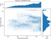 |
Fig. 1 Planets of the NGPPS76 5e9 population model for 1000 stars. We show only planets up to an orbital period of 8 yr, which are of interest for this study. The top panel shows the histogram over orbital period, and the right panel shows the histogram over planet radius. |
2.3 The KM20 planet occurrence rate
Despite recent improvements, the planet occurrence rate from the Kepler data is still not entirely agreed upon. Uncertainty persists due to our limited knowledge of the host star properties, and thus of the planet radius derived from the transit depth. For instance, the Kepler pipeline of transiting planet determinations assumes star-averaged radii for the estimation of the Kepler detection efficiency. This leaves further room for improvement.
In an effort to improve the inference of the planet occurrence rates of FGK stars from the Kepler data, Kunimoto & Matthews (2020) compiled an independent catalog of Kepler planet candidates. They employed the ABC method and included the star-specific radii in the calculation of the detection and vetting efficiencies. Their analysis is based on the Kepler subsample of 116 637 FGK stars with a radius measurement accuracy of 10% or better. For these stars, they searched the Kepler Q1–Q17 database for transit events. They defined an event as a transit candidate when at least three events with a signal-to-noise ratio S/N > 6 were observed. They applied their own vetting procedure to distinguish false positives and false negatives from what otherwise could be considered a planet candidate. With their method, Kunimoto & Matthews (2020) achieved a recovery rate of 99% of the confirmed KOIs and 65% of the candidate KOIs labeled as such in the NASA exoplanet Archive for the same stellar sample. Their planetary sample comprises 2533 planets, which populate 79 out of the 9 × 10 cells in Porb−Rp space between 0.78–400 days and 0.5–16 RE. Compared to Hsu et al. (2019), their detection and vetting efficiency values are lower for S/N values below 16 by up to a factor of a few, yielding lower planet occurrence rates where the S/N is this low. Marginalized over all FGK-type stars and all planets, they arrived at an occurrence rate of  planets per star. Furthermore, Kunimoto & Matthews (2020) did not find a statistically significant planet radius valley over a large Porb range as Fulton et al. (2017) did, but instead found an increased abundance of 2.0–2.8 RE planets. The accumulated estimates for P < 50 and P < 100 agree well in general with previous works that used the inverse detection efficiency method. We used their occurrence rate diagram, which is marginalized over FGK stars, and call our population created from this input data set KM20.
2.4 From occurrence rates to population models
In this section, we describe how we translated the planet occurrence rate into a planet population model similar to the NGPPS data set.
Formally, the occurrence rates of Hsu et al. (2019) and Kunimoto & Matthews (2020) are provided as mean values, and their 1σ uncertainty ranges over a set of cells. Each 2D cell is bounded by a lower and an upper value of Rp and Porb. While the Rp and the Porb grids can be unequally spaced, the 2D grid is rectangular. For each individual cell, the 1σ uncertainties are the maximum values of a possibly asymmetric occurrence rate distribution in that cell. In order to not only recover the mean but also represent its uncertainty in the planet population, we approximated the occurrence rate distributions of each cell as a symmetric Gaussian with 3σ upper and lower limits. For each cell, occurrence rate values were picked randomly until 100 values were admitted in a way to preserve a Gaussian distribution. With 100 draws, we represent the original mean values to within a few percent and the original 1σ uncertainty to within 10%,
Given 1000 stars, an occurrence rate of 1% means that there are 10 planets around these stars on average within the bounding Rp and Porb values of that cell. Our aim is to simulate a relatively large number of planets to ensure that that the cells are approximately equally populated. Therefore, we used three different numbers of input stars per cell. For occurrence rates below 0.2%, we took 50 000 stars (yielding a maximum of 100 planets per cell), for rates below 2%, we took 10 000 stars (yielding between 20–200 planets per cell, and above 2%, this yielded 1000 stars (Np > 20). For cells with only an upper limit, we assumed a uniform occurrence rate distribution between 0 and the upper-limit value, and we represented the population by 2000 stars.
An occurrence rate o in percent and a number of stars Ns yields the number of planets populating that cell as Np = 0.01 × o × Ns. These planets were assigned with a radius value assuming a uniform likelihood and a Porb value assuming a uniform log likelihood within the bounding Porb–Rp ranges of that cell. Finally, each planet was randomly assigned with a starID between 1 and the Ns value for that cell. This implies that we assumed random planet architectures. For the subsequent calculation of the PPY, we kept track of the cell scaling factor Ns. As a result, we obtained a table of planets with the starID, Rp, and Porb value.
This process was repeated 100 times for the 100 occurrence rate representations of each cell, yielding 100 tables. Together, they built the population model given the input occurrence rate diagram. The 100 tables can also be viewed as 100 snapshots of sky observations in time. From the 100 tables, we can calculate the mean occurrence rate of each cell. These values are displayed in Fig. 2 for HSU19 and KM20, respectively.
3 Input stellar samples
The PLATO mission has been designed to monitor a large sample of ≳245 000 K7-F5 dwarf or subgiant stars of magnitude 13 or brighter, observed at 500-1000 nm wavelengths. Out of this P5 sample, a subset of ≳15 000 stars shall be observable at a photometric noise of 50 parts-per-million in 1h (ppmh−1) or better; the subset with magnitude 11 or brighter forms the P1 sample (red book). The figure of 245 000 targets assumes two long-duration observations, possibly separated into the northern and southern hemispheres. According to the nominal mission design, each of the fields will be monitored for transit events over a duration of 2yr. This is the 2+2 mission scenario (red book). An alternative scenario could be to stare at one field for 3 yr and at several other fields for a shorter period of time (e.g., two months) in order to cover a larger portion of the sky during the 4-yr prime mission (the 3+ 1 mission scenario; red book).
A compilation of 2 378 177 stars fulfilling the above criteria and distributed throughout the sky is provided in the all-sky PLATO input catalog asPIC (Montalto et al. 2021). However, only the fraction of stars that falls within the fields of view will actually be observed by PLATO. The PLATO FsoV are of squarish shape and cover about 2000 deg2 of the sky (Nascimbeni et al. 2022; Pertenais et al. 2021). Approximating this shape by a square would yield a solid angle of 49 deg2 according to Nascimbeni et al. (2022), which is 5.15% of the sky. Assuming a uniform distribution of the stars on the sky, we can estimate that each FoV contains 122 476 asPIC stars. This is consistent with the minimum requirement of 122 500 stars at mission level, although the eventually chosen fields in the 2+2 mission scenario may contain 20% more stars (Nascimbeni et al. 2022).
We sorted the stars into magnitude V bins of 5–8, 9, 10, 11, 12, and 13 by rounding the values for Gaia V provided in the catalog without accounting for their uncertainties, which are around 0.2 (Montalto et al. 2021).
We determined the spectral class of each star from their Teff values provided in the asPIC, neglecting the provided 1σ uncertainty σTeff (case 0 × σTeff). We used the relation between Teff and spectral class for main-sequence stars of Pecaut & Mamajek (2013) as presented in their Table 5. If we are to collect KGF stars, we need to define boundaries between K0/G9 and G0/F9 stars, respectively.
Linear interpolation between the classes K0 and G9, which are separated in Teff by 30 K (Pecaut & Mamajek 2013), yields a G to K transition at 5310 K. Linear interpolation between the classes G0 and F9, which are separated in Teff by 120 K, Pecaut & Mamajek (2013), yields an F to G transition at 5980 K. To sort the stars into spectral class, we used these sharp F to G and G to K transitions. The respective upper limit for F-type stars of 7320 K and the lower limit of K-type stars of 3865 K is not important here as the asPIC only contains stars between K7 and F5.
Neglecting the uncertainty  induces an uncertainty in the star count. The individual 1σ uncertainties of a star are around 227 K (Montalto et al. 2021). Taking them into account (case 1 × σTeff) and averaging over 100 iterations, we obtain a 1σ uncertainty in the number of stars in each class of about 0.1% for magnitudes 13 to 12, which increases to 1% for the less abundant magnitude 8 stars. However, the mean values for the star numbers in each class differ from those obtained above, where we neglected σTeff, by more than 3σ in some cases; see Table 1. These differences are more pronounced the more unequal the number of stars in adjacent classes are, and they arise because a higher number of stars are distributed down the slope than upward.
To address a maximum uncertainty in the F to G and G to K transitions, we shifted the first by +120 K and the second subsequently by −30 K. The first modification would decrease the number of F stars over all magnitudes by up to 23% and increase the number of G stars by 22%. The second modification would increase the number of G stars by 3% and decrease the number of K stars by 7%. While spectral classes do not enter the computations of the PPY, they are important when the PPY for a certain stellar class is to be determined.
For comparison, Kunimoto & Matthews (2020) adopted values for F to G and G to K transitions of 6000 K and 5300 K, respectively. Montalto et al. (2021) used a Teff value of 6510 K (3870 K) that is representative of F5 (K7) stars (Pecaut & Mamajek 2013) to limit their sample to K7-F5 stars.
In Table 1, we list the input stars obtained in this way before taking their 5.15% fractions. To sort the spectral type by the effective temperature, we interpolated linearly in the F/G and G/K transition values of Pecaut & Mamajek (2013) and neglected the uncertainty in Teff (0 × σ). For comparison, we show the included case (1 × σ).
Taking a fraction of 5.15% of the stars of the asPIC as done in this work is equivalent to assuming a random pointing direction of PLATO. In Table A.1, we compare this stellar sample from a random pointing direction with the pointing directions of LOPN1 and LOPS1 defined in Nascimbeni et al. (2022).
While the LOP1 fields contain 26-30% more stars than the P5 requirement, we find 32-35% more stars in these pointing directions that satisfy the P5 sample criteria. We also find that these fields contain disproportionally more F stars and more faint stars than the average sky field. As at the current stage the final pointing direction is not yet fixed, we consider a random pointing a more robust approach than using a specific field for estimating the PPY.
Finally, we binned the stars into about 100 radius bins of constant width 0.05 Rsim. Figure 3 shows the normalized histograms of stellar radius after our sorting for stellar class and magnitude.
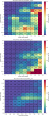 |
Fig. 2 Inferred planet occurrence rates (color code) for the NGPPS76 5e9 population model (top) and mean values from 100 iterations for Hsu19 (middle) and KM20 (bottom panel), where we used the grid in orbital period and planet radius as in the original work, but the same color-coding for all three data sets. |
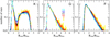 |
Fig. 3 Histograms of the asPIC stars normalized to 1 and sorted for spectral class and apparent magnitudes between m = 8 to 13 (color code as labeled). |
Number of stars in the asPIC catalog according to our sorting.
4 Detection efficiencies
The planet yield of a transit survey such as Kepler or PLATO depends on several factors, including the detection efficiency of the search methods applied in the data pipeline (see, e.g., Christiansen et al. 2020).
The detection efficiency can be parameterized as a function of the S/N. The signal is the measured transit. It is characterized by the transit depth (proportional to the radius ratio), its duration (proportional to the orbital period), and the number of observed transits (constrained by the observational strategy). The noise includes photon noise from the target, but also residuals from instrumental noise and stellar variability.
The PLATO space telescope is equipped with 24 normal cameras. They are separated into four groups, which overlap each other in their viewing angle. When detection efficiencies are calculated, it is important to estimate how many cameras observe any given target.
The PLATO payload is required to achieve an overall reliability >79% at the end of the extended mission lifetime (6.5 yr). In order to account for the aging of the instrument and possible failures of hardware components, we defined two scenarios. At the begin-of-life, the instrument has full performance and 24 operational cameras. At the end-of-life, the photometric performance has degraded (e.g., because of lens darkening or because of radiation damage of the CCDs) and up to 2 cameras might have failed and may not deliver any data. Consequently, the free parameters added to our detection efficiency model are i) eight different numbers of cameras for a begin (24, 18, 12, 6; BOL) and end-of-life (22, 17, 11, 5; EOL) scenarios, ii) a stellar magnitude range between V 8 and 13, iii) the mission durations (0.1667, 1, 2, 3, 4, 6, and 8 yr), and iv) the stellar types (F, G, K, and M).
4.1 Relation between detection efficiency and signal-to-noise ratio
The detection efficiency can be approximated as a simple function of the S/N with a finite-size threshold. Below the threshold, no planets are detected. Above the threshold, a certain fraction of planets is detected. In between, a smooth transition can be created by linear interpolation (see Jenkins et al. 1996, 2010, but also Hsu et al. 2019; Kunimoto & Matthews 2020; Christiansen et al. 2020).
For Kepler, Fressin et al. (2013) suggested that the threshold should be between S/N = 6 and 16, where above the latter, 100% of the planets should be detectable. These limits are more conservative than previous calculations from the PLATO definition study report, which used an upper boundary of S/N = 10. For consistency with the previous PLATO estimates, we adopted the values from the red book.
4.2 Signal and noise models
The S/N is the ratio of the transit depth δ, functioning as the received signal, and the noise N. The transit depth is calculated by

where R* is the stellar radius. Other geometrical parameters such as impact parameter or limb darkening, which influence the transit depth, are not considered in this work.
The noise can be addressed with the help of the effective combined differential photometric precision CDPPeff , as outlined below. The noise

is given in ppm h−1, but is dimensionless. The number of transits Ntransits is calculated with the mission duration tmission, the orbital period of the planet, and the transit duration ttransit,


The semi-major axis α is calculated with Kepler's third law (Eq. (4)), where G is the gravitational constant, and M, is the mass of the star. The mass of the planet Mp is neglected here because Mp ≪ M*. For large numbers of transits, a common approximation is

We requested a minimum number of transits of two before a signal was classified as a transiting planet. For instance, assuming a planet has Porb = 1.5 yr and tmission = 2 yr, Eq. (5) yields, and thus the planet would be classified as a nondetection, although two transits could take place within 2 yr. Therefore, we also took the timing of the first transit, t0, and the transit duration into account. As t0 is not known, we generated 100 random numbers with a uniform distribution for t0 within the interval 0–Porb. If:

the number of transits increases to Ntransits + 1 . This occurred in n+1 cases. We assigned the probability of n+1/100 of observing one additional transit. We verified that the resulting probability is well converged for the choice of 100 random numbers.
The consideration of the timing of the first transit is particularly relevant for long-period planets such as Earth around Sun-like stars, which have only a small number of transits within a few years of uninterrupted observation time.
4.3 CDPPeff and the noise model
The PLATO mission consortium has developed tools and models to assess the expected performance of the PLATO instrument. They can be used to predict the measured flux and the expected noise at pixel level and at mission level for a given star. The noise budget of the PLATO light curves can be approximated with a model that includes photon noise from the target, spacecraft jitter, and read-out and background noise. An additional noise parameter is the stellar variability σ*. This simplified model is appropriate for estimating the detection efficiency for a planet detection. We express the noise budget as the CDPPeff in ppmh−1 (the noise in ppm for a signal that is averaged over 1h), although its dimension is  . The relevant timescale is represented by the transit duration in hours,

The first three terms are collectively labeled CDPP, so that

Jitter describes the noise that is produced by small-amplitude high-frequency movements of a satellite (Drummond et al. 2006). This error source affects the geometric accuracy of highresolution satellite imagery (Pan et al. 2017). For the Transiting Exoplanet Survey Satellite (TESS), Ricker et al. (2014) pointed out that the most important source of systematic noise is due to jitter, while other noise sources decrease with the brightness of the observed star. For PLATO, jitter is estimated to be the dominant noise source at V < 9 (Cabrera et al., in prep.). We write the jitter noise as σjitter = kjitter with kjitter = 10 ppmh−1 (Cabrera et al., in prep.).
The CCDs work by amplifying the voltage induced by the electrons that were lifted into the conduction band after the absorption of photons in an array of pixels. The accumulated charge of the electrons in a pixel is read out before the pixel can be exposed to the light source again. However, the measurement of the electron charge and thus the number of electrons is imperfect. This instrumental noise source is called readout noise and is given as the number of electrons (Richmond 2004). We considered readout noise to be mixed with background noise (caused by background stellar contaminants or stray light) up to a value of kreadout = 4 × 57.8 electrons (Cabrera et al., in prep.). The values for kjįtter and kreadout may be subject to change in the course of progress in the understanding of the PLATO instrument performance. The value of kreadout is provided in electrons, but it has to be combined with the other quantities that at system level are presented in ppm. For the estimate of the impact of the readout noise at system level, we assumed that it is not correlated in time or among cameras, hence

Electronics readout and background noise are the leading noise source at the faint end (V > 13 ).
Photon noise is a fundamental form of uncertainty in the measurement of light, inherent in the quantized nature of light (Hasinoff 2014). As emission of photons from a star is a spontaneous process, the uncertainty of the number of photons hitting the detector increases with the square root of the signal, which is the flux ƒ of incoming photons per unit area. The photon noise is expressed as a noise-to-signal ratio  so that
  . This stellar incoming flux changes with apparent magnitude m as

where ƒmag11 is our reference point for an magnitude 11 star. The electronic devices of the spacecraft are designed to yield an accuracy of CDPP = 50 ppmh−1 for an m = 11 star observed by 22 cameras (EOL) simultaneously. We ensured this requirement by the choice of ƒmag11 = 1.6 × 10⁵ (Cabrera et al., in prep.).
The stellar variability σ* was set to 10 ppm in 1h following the approach for Kepler, with its white noise being 10 ppm for a 12th magnitude G2V planetary target star (Van Cleve & Caldwell 2016).
Figure 4 illustrates the noise CDPP in dependence on the apparent stellar magnitude and the assumed number of cameras observing the target.
Finally, we can calculated the S/N and interpolated the detection efficiency (DE) from this. While in the simulation, we calculated DE values for the individual planet-star combinations, we show in Fig. 5 the detection efficiency on a grid of Rp and Porb values for illustrative purpose specifically for a magnitude 11 G star and an observation time of 2 yr.
5 Planet Yield for PLATO Estimator
The tool called Planet Yield for PLATO estimator is a Python program for the determination of the number of planets that can be detected, given a planet population model, a sample of stars that shall be observed, and the characteristics of the detection efficiency. The development of PYPE has been heavily inspired by and benefited from the open-source program Exoplanet Population Observation Simulator (EPOS) of Mulders et al. (2018, 2019), which we used initially.
The basic approach of PYPE is structured as follows:
- (i)
Defining a planetary population model. Orbital period values are converted into orbital distance and vice versa, assuming a planet mass Mp = 0 unless the Mp values are provided with the population model, which is the case for NGPPS.
- (ii)
Defining a stellar sample to be observed. If the number of stars to be observed (M*,obs) exceeds the number of systems with planets Nsys in the planet population model by a factor of two or more, identical copies of the planetary systems are made to approximate N*,obs. The following steps are thus made for a number of stars m × Nsys, m ≥ 1. This idea has been adapted from the EPOS code. Here, we used 5.15% of the number of stars from Table 1 and scaled the resulting PPY down to 5.15% to account for the effective FoV of PLATO, as discussed in Sect. 3.
- (iii)
The next step is to separate the transiting from the non-transiting planets. This step is purely geometric and calculates the probability of a transit using
where R* is one of the binned R* values. If the geometric transit probability ƒgeo is greater than a random variable e [0, 1], the transit occurs. Unlike the EPOS code, which does take care of mutual inclinations between planets in the same system, we neglected information on planetary architectures. This perhaps unnecessary simplification matters when only a few systems are observed, but it will average out when many systems are observed. We may therefore underestimate the uncertainty in the PPY when the PPY is low.
- (iv)
We separated detected and nondetected transiting planets using the detection efficiencies of PLATO (Sect. 4), which adopt values between fdet = 0 and 1 (100%). If a random value ϵ [0, 1] is lower than fdet, the planet is counted for the PPY. In steps (iii) and (iv), the stellar radius distribution matters most.
- (v)
While we ensured that the planets have semi-major axes a greater than 1 R*, observed ultrashort-period planets are found to be limited to a/R* > 2 (Adams et al. 2021) and to be small. Larger gaseous planets may be more readily subject to Roche-lobe overflow, and disintegrate. By neglecting these constraints, we slightly overestimate the PPY for planets at small orbital distances.
- (vi)
The obtained PPY is scaled from the simulated number of stars, m × Nsys, to Nobs. The PPY obtained from PYPE in this way is valid for a given single-mission duration, number of cameras, stellar class, stellar magnitude, and a single input population model.
- (vii)
After-PYPE: The complex lotus-shaped FoV is taken into account. PLATO does not observe the whole FoV with all cameras simultaneously. Instead, different fractions of the field are observed with 6, 12, 18, or 24 cameras. We multiplied the PPY with a factor that stands for the percentage of the FoV observed by each number of cameras. For example, only 13.79% of the FoV are observed with 24 cameras, meaning that the results for the computation with 24 cameras was multiplied by 0.1379.
- (viii)
The above steps were repetitively executed for different mission durations, spectral class, and stellar magnitude.
- (ix)
The entire process was repeated 10 × (NGPPS) or 100 × (HSU19, KM20) in order to estimate the 1σ uncertainties and the mean values of the PPY.
- (x)
Finally, the PPY was sorted into Rp and Porb bins. We adopted the classification of planets according to their radius similar to Fressin et al. (2013) (see Table 2), which precedes the finding of a radius gap at 1.5–2.0 in the Rp–incident flux relation (Fulton et al. 2017).

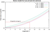 |
Fig. 4 Noise model for a begin-of-life scenario with four camera configurations (6, 12, 18, and 24 cameras). The dotted red line shows the reference point of 50 ppm h−1 for a magnitude 11 star. |
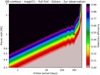 |
Fig. 5 Example detection efficiency contour grid observing an 11 magnitude G star for 2 yr with 24 cameras. |
Planet radius bins for the PPY.
6 Results
Our calculations with PYPE for an estimate of the PPY have led to an immense amount of data regarding the number of detected planets as a function of mission duration, stellar radius, stellar magnitude, and planet type. The following graphs in this section display only a small portion of the results. Figures similar to Fig. 8 displaying the results for other parameter choices as well as comprehensive data tables of PPY as a function of magV, mission duration, stellar class, and planet type can be found in more detail in the online repository3.
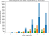 |
Fig. 6 Number of detected planets for given magnitude range for NGPPS (blue), HSU19 (orange), and KM20 (green). The darker bars show planets <2 RE , and the lighter bars show planets >2 RE. Every bar represents the PPY for BOL. |
6.1 Planet yield dependence on free parameters
In Fig. 6, we plot the PPY in dependence on the stellar magnitude for a 2+2 mission scenario and BoL. We find that most planets will be detected around magnitude 12 stars, followed by stars of magnitude 13 and 11. The relative behavior of PPY over magnitude V is similar for all three population models (green, orange, and blue); strong differences occur in absolute numbers. The majority of planets are detected around fainter stars (V > 11), while the RV-feasible planets (V ≤ 11) make up between 38% and 49% of detections. The PPY ratios of these two magnitude groups are 2.4 (NGPPS), 2.1 (HSU19), and 2.6 (KM20).
6.2 Detectable planet occurrence rates
Figure 7 shows the PPY subdivided into planet type and orbital period bins for the 2+2 yr and 3+1 yr mission scenarios. For most bins, the 3+1 yr case yields a higher planet count than the 2+2 yr case. The larger a planet and the shorter its orbital period, the more strongly the PPY benefits from the 3+1 case. This is because in the 3+1 case, seven different fields are observed and thus a larger number of different planets, which can be rather quickly detected with two transits when they are on short orbital distance and large.
The opposite holds for smaller and more distant planets with an orbital period greater than 50 days (i.e., approaching two months). Clearly, in the +1 short-duration case, Earth-size planets in the HZ cannot be found when the FoV is changed every two months. On the other hand, smaller planets on long orbital periods benefit from a third year of continuous observations of the same field as compared to only 2 yr. Together, these opposing effects lead to a ∼50% higher PPY in the 2+2 than in the 3+1 case when the orbital period exceeds one month.
The PPY between the NGPPS population and the HSU19-KM20 populations shows large Rp, Porb specific differences. For instance, with NGPPS, we estimate the detection of ∼6320 hot Neptunes in 2–5 days, whereas with HSU 19 and KM20, we estimate only ~550 and ~420, respectively. For earths in the 250–500 days bin, which partially overlaps with HZs of GK stars, we see a different picture. There, the highest PPY is found with the HSU 19 population in the amount of 24 ± 4, followed by NGPPS with ~6.6 ~ 1.0, and KM20 with only 0.7 ± 0.4 planets. Planet yields for orbital periods greater than 500 days are at zero for HSU 19 and KM20 because the given occurrence rates do not cover this area.
In Fig. 8, we show an example in which the PPY is subdivided according to stellar type. This particular example is for a 2+2 yr mission scenario with the HSU 19 population, but the same pattern is seen for every possible constellation of planet populations and mission scenarios. The tables for other parameter choices can be found in the online repository.
Figure 8 shows that G stars generally have the greatest number of planets flagged as detections, followed by F stars and К stars, except for small planets at wide orbits. F stars have the highest abundance in the PIC catalog, followed by G and K stars. However, the transit depth of small planets around F stars is lower than for K stars. The low signal for F stars can be compensated for by a low noise level, which can be achieved by multiple transits and thus is possible for short-period planets, but not for long-period planets. Thus for the latter, the deeper transit in front of K stars leads to more detections of small planets, even though K stars are less abundant in the PIC catalog. Furthermore, for HSU 19 and the 2+2 case, which we argued above is more favorable to detecting earths at wide orbits, we obtain a maximum of a dozen ±2 detected Earth-size planets around G stars in the 250–500 days period bin. While agreeing with the value of 11 detected Earth-size planets in the conservative HZ around Sun-size stars predicted by Heller et al. (2022) for a 2+2 mission scenario, we add a word of caution as the assumptions behind both studies are very different. Heller et al. (2022) assumed 2 × 7500 bright bright (mag V ≤11) stars, corresponding to the P1 sample, and a higher true ηE of 37%, whereas our estimate is derived from the larger but on average fainter P5 sample and a lower ηE of 16–28%. Our estimated value decreases by 20% when changing to a 3+1 yr mission. For NGPPS, we find 3.7 ± 0.7 , and for KM20 0.3 ± 0.3 for a 2+2 yr case.
When we allow for a planet radius up to 2RE (as for habitable planets in the PLATO definition study report), we estimate the planet yield around G stars to be 100 ± 7, 42 ± 3, and 1.6 ± 0.7 for HSU19, NGPPS, and KM20 in the 250–500 days period bin, respectively.
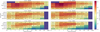 |
Fig. 7 PPY as a function of binned planet size and binned orbital period for NGPPS (top row), HSU19 (middle), and KM20 (bottom), and for a 2+2 mission scenario (left) or a 3+1 mission scenario (right). |
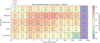 |
Fig. 8 PPY as a function of binned planet size and binned orbital period for the 2+2 yr mission scenario and the HSU19 population around F (red), G (green), and K stars (blue). |
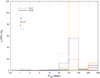 |
Fig. 9 Relative change in the statistical mean values of the PPY that results from the inclusion of planets that are observed to transit only once. Results are presented for the HSU19 planet occurrence rate and the 2+2 (solid) or the 3+1 (dashed) mission scenarios at BOL for Jupiters (J, yellow), Neptunes (N, blue), Super-Earths (sE/mN, brown), Earths (E, green), and Sub-Earths (subE, gray). |
6.3 Single-transit detections
The results presented so far were obtained under the premise that at least two transits are observed by PLATO, in accordance with the definition study report. However, single-transit events will occur. In this section, we quantify the increment in the PPY that arises from single-transit events.
Figure 9 shows the relative increment of the statistical mean value of the PPY that results from the inclusion of planets that are observed in transit only once.
Small positive or negative fluctuations in the relative change can occur, which result from the 1 σ uncertainties of the statistical means. These fluctuations are lower than 1% for most Porb–Rp bins. Because negative values are solely due to this statistical uncertainty, only positive changes are shown.
A statistically significant change can occur if 0.5 < Porb/tmission < 1 (case i) or if Porb > tmission (case ii). In the first case, two transits might have been observed by PLATO, but due to unfortunate timing of the first transit, the second one is missed. Half of the planets with such an orbital period will appear as single-transit events on average, while the other half will appear with two transits, and will be detected or not detected according to their DE. In the second case, PLATO can see one transit at most.
As expected, Fig. 9 therefore displays an increment in the PPY when cases i or ii apply. In the 2+2 mission scenario (solid lines), the increment adopts statistically relevant values only in the longest-period bin, where both cases apply. As larger planets have a better DE, their detectability with only one transit is higher, and thus their PPY benefits more than that of smaller planets. For Neptune- to Jupiter-size planets, the PPY increases by 9–13%, given the input occurrence rate. It is clear that transit detections of extrasolar Neptune- and Jupiter-analogs in terms of Rp and Porb can only occur via single-transit events.
The largest increments of up to a factor of two are obtained for the 3+1 mission scenario. As they occur for Porb within 20–100 days, these strongest increments entirely result from the step-and-stare phase. A much smaller increment of up to 5% is seen in the 250- to 500-days bin, which results from the 3-yr observing phase.
This study emphasizes the importance of single-transit detections for the study of the architecture of Solar System analogs. Further figures for different mission scenarios and planet populations can be found in the Online repository.
6.4 Planet yield of LOPN1 and LOPS1
While the definite FoV for PLATO has not yet been chosen, Nascimbeni et al. (2022) has proposed two fields for the long-observation phases. One lies in the northern (LOPN1) and the other in the southern (LOPS1) ecliptic hemisphere. Taking the same pointings for PLATO as that study and cross-referencing it with the asPIC from Montalto et al. (2021), we obtain 165 351 and 161631 stars for LOPN1 and LOPS1, respectively. These stars underwent the same treatment as the asPIC in Sect. 3. The PPY was calculated for the HSU19 population for a 2+2 yr mission scenario as a 3+1 yr mission would not qualify because the additional +1 yr period would not be a long observation, but a step-and-stare phase that changes the pointings every two months. For the 2+2 yr mission, the first 2 yr calculation was made with LOPN1 and the second with LOPS1. The results in Fig. 10 for the nominal pointings LOPN1/LOPS1 can be compared directly with the results from Fig. 7 for a random pointing. The nominal pointings yield a larger number of planets, but it is not dramatically different, as the expected result of the optimization criteria used in the selection of the PLATO pointing fields (see Nascimbeni et al. 2022 for details).
7 Discussion
The scenarios presented here primarily studied the current baseline observing duration of 4 yr (as constrained by the ESA schedule planning) and the scenarios as addressed in the red book. We recall that PLATO is designed for a 6-yr observing duration and will have consumables for up to 8 yr of operations. To take advantage of these options, mission extensions can be applied for after launch of the mission. These scenarios deserve further studies that are currently ongoing.
NGPPS model. With input occurrence rates a factor of a few higher than that of HSU19, NGPPS unsurprisingly predicts the largest PPY. Thus, the bulk PPY from NGGPS model appears to represent the high end of expectations for the PLATO mission. However, it necessarily makes a number of simplifying assumptions. Every planetary system in the NGPPS model is assumed to form and evolve around a Sun analog with a mass of 1 MSun. This does not reflect the variety of stars that will be observed. Planetary systems formed around stars of different mass and metallicity are observed to exhibit different architectures. Moreover, some planets may have formed by means other than core accretion, as indicated by the recent combined ALMA and HST observations of a few million years old young protostellar disk (Currie et al. 2022). A pathway to understand planet formation could be to compare different predictions to the observed planet yield.
HZ. The location of an HZ is still a matter of ongoing debate as it depends on our understanding of the stellar flux (Ahlers et al. 2022), the effect of clouds in the planetary atmosphere (Leconte et al. 2013), and of geological processes such as plate tectonics and the temperature-stabilizing carbon cycle (Kruijver et al. 2021), although the ability to sustain liquid water on the surface is commonly considered a necessary condition for habitability.
The HZ of a planet could be calculated with the effective temperature and luminosity of its host star and a model for the radiation transport in the planetary atmosphere (Kopparapu et al. 2013; Kopparapu et al. 2014). Uncertainties then result from the global mean properties such as atmospheric composition, in particular, the abundance of greenhouse gases, and from opacities. Kopparapu et al. (2013) related the CO2 abundance to incident flux at the top of the atmosphere. Conditions satisfying the criterion for liquid water at the bottom of the atmosphere result in a conservative habitable zone of 0.99–1.70 AU for the Sun. Kopparapu et al. (2013) provided a relation to estimate the HZs of other stars. Calculating a specific habitable zone for every individual star (Bryson et al. 2021) would exceed the scope of this study. Given the uncertainties, we are only interested in estimates here. Assuming representative values for the effective temperatures (5000, 5800, and 6500 K) and stellar radii (0.7, 1, and 1.3 Rsun), we can calculate the HZs of 153–358, 340–797, and 733–1678 days for KGF stars, respectively. With KM20 and HSU19, which only reach orbital periods of up to 400 and 500 days, respectively, the HZ around K stars is fully covered, while the G-star HZ is only partly covered and the F-star HZ is entirely missed.
Using NGPPS, we estimate that PLATO can find one planet there when the monitoring duration is limited to 3 yr. Given the closer-in HZ boundaries around K stars, we estimate that PLATO can detect a few (KM20) to a few dozen planets in the 0.8–1.25RE size range. These numbers increase quadratically if larger planets are admitted. Bryson et al. (2021) considered planets up to 1.5RE for their η⊕ estimate, while in the red book, radii of even up to 2 RE are considered.
Comparison to the red-book results. An earlier study (red book) predicted a total planet yield for planets around stars with magnitudes of V ≤ 13 to be ∼4600 and ∼11000 for the mission scenarios 2+2 yr and 3+1 yr. Our most conservative population KM20 predicts PPYs being respectively ∼70% and ∼32% higher than this. The NGPPS population exceeds the red-book estimates by a factor of 10 and 7.5. In the previous study, the estimates were based on the occurrence rates by Fressin et al. (2013), which are given there for similar planet types, but only an orbital period range of 0.8 to 85 days. This means that various assumptions regarding the occurrence rates of more distant planets have been made. Our estimates fill these unknowns with observational and theoretical values, showing that the previous assumptions were highly conservative.
RV feasibility. The brightness of a star determines the possibility of constraining the bulk properties of exoplanets. The fainter the star, the lower the likelihood of providing accurate planet parameters for a detected exoplanet through RV measurements. Figure 6 shows that the majority of detected planets are found for magnitude V > 11 stars and are therefore too faint for their follow-up RV measurements. Nonetheless, the number of detections around V ≤ 11 stars is still impressive compared to the 1228 already found and confirmed exoplanets at V ≤ 11 (NASA Exoplanet Archive, May 23, 2022). An objective of PLATO is to detect planets around stars with brightness V ≤ 11. With the presented estimates, this goal will be achieved for one-third of the planets, and following RV measurements will be enabled.
Rediscoveries. PLATO will detect several thousand planets. The question then is how many of these are already classified as candidates or confirmed planets by other space missions and ground-based observations. The Kepler FoV could be within one of PLATOs long-duration FsoV, depending on the final pointing strategy chosen by the PLATO team (Nascimbeni et al. 2022), meaning that a decent number of Kepler and K2 exoplanets will probably be rediscovered. However, TESS observed approximately 30000 deg2 of the sky for a minimum of 27.4 days (Howard 2015). Figure 11 shows the TESS project candidates4 (by 2022 May 13) that are similar in planet type and orbital period bins to Fig. 7 and distinguished for the status of confirmation, which is either candidate, false positive, confirmed (meaning verified through additional observations using other telescopes), or previously known planets that were discovered by other missions before TESS. As most of the TESS FoV is observed only up to 27 days, the majority of the candidates are found at short orbital periods; the TESS planet yield peaks for hot Jupiters. From the number of objects already evaluated to count as confirmed or a false positive, we estimate that 150 out of the 860 current hot-Jupiter candidate TESS planets may later be confirmed as planets. Together with the previously known hot Jupiters, the number of 314 previously known hot Jupiters is with a factor 0.5–3 about the same as our PPY estimate. This means that a significant fraction of the hot Jupiters to be found by PLATO will probably be rediscoveries. It should be noted that planets discovered by TESS include planets around M stars, which are not included in the star sample studied in this paper (although PLATO will observe M stars as part of the P4 population; see Montalto et al. 2021). For an estimate of the TESS-expected yield through the prime and extended missions, see Kunimoto et al. (2022).
Single-transit events. Single-transit events can occur if Porb > 0. 5tmission. In the 2+2 yr case, this applies to planets with Porb > 1 yr. In the respective bin of 250–500 days, an increment up to 14% is indeed seen. Although this is small, it suggests that an analysis of single-transit events may reveal planets at longer orbital distances that otherwise would be discarded, where the true occurrence rate is still highly uncertain.
For the 3+1 yr case, a strong PPY increase occurs at orbital periods of 20–100 days as it benefits from the step-and-stare phase (6 times two months) of this mission scenario. Lowering the Ntransits threshold enables us to detect some planets that were previously discarded. The detection of Earth-Sun analogs does not seem to profit from this change as other parameters such as the planet radius seem to play a stronger role.
On the other hand, even a few detections at wide orbital distances would be valuable for building up a data base for the occurrence rate of planets at wide orbital distances. This will have to be set up over decades and by combining single-transit observations from various missions such as Kepler, TESS, or NGTS. Even partial single-transit events from different observing programs might be combined that otherwise remained undetected. This may help to detect Earth-Sun analogs.
The LOPN1 and LOPS1 stellar fileds. By comparing the PPY using the average stellar sample with that obtained with LOPN1 and LOPS1, we see that the former results amount to about two-thirds of the LOPN1/LOPS1 results. The number of stars that were used show the reason for this. Scaling the 2 374 623 stars in the asPIC down to 5.15% (to account for the FoV size of PLATO in a given random pointing direction) and assuming a uniform distribution leaves us with 122 293 stars in each field. Observing two fields means 244 586 stars, which is about two-thirds of the 326982 stars of LOPN1+LOPS1. This is an expected consequence of the field optimization criteria used in Nascimbeni et al. (2022).
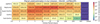 |
Fig. 10 BOL-PPY as a function of binned planet size and binned orbital period for the HSU19 population and the 2+2 yr mission scenario using the LOPN1 and LOPS1 stellar catalog. |
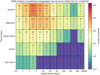 |
Fig. 11 TESS exoplanets as a function of planet type and orbital period, separated into planet candidates (black), false positives (red), previously known planets discovered by other missions than TESS (blue), and confirmed planets verified through additional observations using other telescopes (green). |
8 Conclusion
We have applied three different input occurrence rate estimates, information on the stellar distribution to be observed by PLATO from the asPIC catalog, and a noise model to estimate the PLATO planet yield as a function of planet size, orbital period, mission duration, and stellar magnitude. Our conclusions from this study are listed below.
The largest unknown in our model is the true number of planets regarding their sizes and orbital periods. We implemented the combined knowledge from real observational data and the most sophisticated theoretical model up to date to solve this problem. Both Kunimoto & Matthews (2020) and Hsu et al. (2019) relied on observational data acquired by the NASA Kepler mission. However, they covered only occurrence rates up to orbital periods of 400 and 500 days, respectively, while the core-accretion planet formation model NGPPS (Emsenhuber et al. 2021a) contains planets out to 2.7 yr. The bulk planet yields reach ∼4000 (KM20), ∼6000 (HSU19), and ∼24000 after 2 yr of uninterrupted monitoring. These rather large differences suggest that the uncertainty in the current PPY estimates might be as large as a factor of a few. The uncertainty from the number of stars contributes less than 20%, and the aging of the camera pixels (BOL versus EOL) contributes less than 10%.
We wish to stress that using a prediction from planet formation models offers a unique possibility to validate these models against observations. The PLATO mission will deliver constraints to improve planet formation models.
We find that a 3+1 scenario compared to a 2+2 scenario increases the PPY by roughly a factor of two with a significant difference depending on orbital distance. To detect Earth-size planets with an orbit duration of about 1 yr (our 250–500 days bin), the 2+2 case leads to a 50% higher yield.
More planets can be detected around fainter stars of magnitude 12 or 13 compared to the brighter ones of magV 11 or brighter, which are more favorable to RV follow-up observations. The PPY ratios of these two magnitude ranges are 2.4 (NGPPS), 2.1 (HSU19), and 2.6 (KM20).
We caution that the detection efficiency model may be subject to improvement in the course of mission preparation and after delivery of the first observational data from PLATO. Our procedure for computing the PPY can readily be adapted to other missions provided the detection efficiencies.
The final observing mission scenario will be determined 2 yr before launch (see “red book”). This study provides a valuable assessment of PLATO’s future mission performance and thus can facilitate this selection process.
Acknowledgements
We warmly thank C. Mordasini for access to the NGPPS model prior to publication and for his comments and insight into the analysis which improved our scientific results. We thank G. Mulders for the provided support with the EPOS code, G. Piotto for access to a preliminary PIC data base, and S. Udry for useful discussions on the scientific results that improved their interpretation. We thank the “transit” group at the EPA department of the Institute of Planetary Research at DLR for fruitful discussions. This work presents results from the European Space Agency (ESA) space mission PLATO. The PLATO payload, the PLATO Ground Segment and PLATO data processing are joint developments of ESA and the PLATO Mission Consortium (PMC). Funding for the PMC is provided at national levels, in particular by countries participating in the PLATO Multilateral Agreement (Austria, Belgium, Czech Republic, Denmark, France, Germany, Italy, Netherlands, Portugal, Spain, Sweden, Switzerland, Norway, and United Kingdom) and institutions from Brazil. Members of the PLATO Consortium can be found at https://platomission.com/. The ESA PLATO mission website is https://www.cosmos.esa.int/plato. We thank the teams working for PLATO for all their work. This research has made use of the NASA Exoplanet Archive, which is operated by the California Institute of Technology, under contract with the National Aeronautics and Space Administration under the Exoplanet Exploration Program.
Appendix A Average asPIC field versus LOPN1 and LOPS1
We derived the number of stars in the pointing directions of the LOPN1 and LOPS1 fields (Nascimbeni et al. 2022) by fixing the rotation of the payload to the pointings (YPLM pointing toward the north galactic pole). Then we determined whether the stars fall in the PLATO FoV.
In our derivation of the LOPN1 and LOPS1 fields, we obtain overall +6, 545 (+4.1%) and +6, 992 (+4.5%) more stars, respectively, than in the P5 sample according to Table 2 of Nascimbeni et al. (2022). As Table A.1. shows, there are disproportionally more F stars and more faint stars in these pointing directions than on the average sky.
Number of stars in percent in the LOP1 fields
The number of stars is given in percentage deviation to 5.15% of the respective number of stars in the asPIC according to our sorting for n = 0; see Table 1. N denotes LOPN1, and S denotes LOPS1.
With most of the PPY estimated to occur around magnitude 11–13 stars (Figure 6) and around F and G stars (Figure 8), the values in Table A.1. suggest a PPY enhancement by 30–40% if these particular pointing directions were adopted.
References
- Adams, E. R., Jackson, B., Johnson, S., et al. 2021, PSJ, 2, 152 [NASA ADS] [Google Scholar]
- Ahlers, J. P., Fromont, E. F., Kopparappu, R., Cauley, P. W., & Haqq-Misra, J. 2022, ApJ, 928, 35 [NASA ADS] [CrossRef] [Google Scholar]
- Alibert, Y., Mordasini, C., Benz, W., & Winisdoerffer, C. 2005, A&A, 434, 343 [NASA ADS] [CrossRef] [EDP Sciences] [Google Scholar]
- Batalha, N. M. 2014, PNAS, 111, 12647 [NASA ADS] [CrossRef] [Google Scholar]
- Borucki, W. J., Koch, D., Basri, G., et al. 2010, Science, 327, 977 [Google Scholar]
- Bryson, S., Kunimoto, M., Kopparapu, R., & etal. 2021, AJ, 161, 36 [Google Scholar]
- Charbonneau, D., Brown, T., Latham, D., & Mayor, M. 2000, ApJ, 529, L45 [Google Scholar]
- Christiansen, J. L., Clarke, B. D., Burke, C. J., et al. 2020, AJ, 160, 159 [NASA ADS] [CrossRef] [Google Scholar]
- Currie, T., Lawson, K., Schneider, G., et al. 2022, Nat. Ast., 6, 751 [NASA ADS] [CrossRef] [Google Scholar]
- Drummond, R., Vandenbussche, B., Aerts, C., Fialho, F. D. O., & Auvergne, M. 2006, PASP, 118, 874 [NASA ADS] [CrossRef] [Google Scholar]
- Emsenhuber, A., Mordasini, C., Burn, R., et al. 2021a, A&A, 656, A69 [NASA ADS] [CrossRef] [EDP Sciences] [Google Scholar]
- Emsenhuber, A., Mordasini, C., Burn, R., et al. 2021b, A&A, 656, A70 [NASA ADS] [CrossRef] [EDP Sciences] [Google Scholar]
- Fressin, F., Torres, G., Charbonneau, D., et al. 2013, ApJ, 766, 81 [NASA ADS] [CrossRef] [Google Scholar]
- Fulton, B. J., Petigura, E. A., Howard, A. W., et al. 2017, AJ, 154, 109 [Google Scholar]
- Gaia Collaboration (Brown, A. G. A., et al.) 2018, A&A, 616, A1 [NASA ADS] [CrossRef] [EDP Sciences] [Google Scholar]
- Hasinoff, S. W. 2014, in Computer Vision: A Reference Guide, ed. K. Ikeuchi (Boston, MA: Springer US), 608 [CrossRef] [Google Scholar]
- Heller, R., Harre, J.-V., & Samadi, R. 2022, A&A, 665, A11 [NASA ADS] [CrossRef] [EDP Sciences] [Google Scholar]
- Howard, A. W. 2015, J. Astron. Telescopes Instrum. Syst., 1, 014003 [Google Scholar]
- Hsu, D., Ford, E., Ragozzine, D., & Morehead, R. 2018, AJ, 155, 205 [NASA ADS] [CrossRef] [Google Scholar]
- Hsu, D. C., Ford, E. B., Ragozzine, D., & Ashby, K. 2019, AJ, 158, 109 [NASA ADS] [CrossRef] [Google Scholar]
- Jenkins, J. M., Doyle, L. R., & Cullers, D. 1996, Icarus, 119, 244 [NASA ADS] [CrossRef] [Google Scholar]
- Jenkins, J. M., Caldwell, D. A., Chandrasekaran, H., et al. 2010, ApJ, 713, L87 [Google Scholar]
- Kopparapu, R. K., Ramirez, R., Kasting, J. F., et al. 2013, ApJ, 765, 131 [NASA ADS] [CrossRef] [Google Scholar]
- Kopparapu, R. K., Ramirez, R. M., SchottelKotte, J., et al. 2014, ApJ, 787, L29 [Google Scholar]
- Kruijver, A., Höning, D., & van Westrenen, W. 2021, PSJ, 2, 208 [NASA ADS] [Google Scholar]
- Kunimoto, M., & Matthews, J. M. 2020, AJ, 159, 248 [NASA ADS] [CrossRef] [Google Scholar]
- Kunimoto, M., Winn, J., Ricker, G. R., & Vanderspek, R. K. 2022, AJ, 163, 290 [NASA ADS] [CrossRef] [Google Scholar]
- Leconte, J., Forget, F., Charnay, B., Wordsworth, R., & Pottier, A. 2013, Nature, 504, 268 [Google Scholar]
- Mayor, M., & Queloz, D. 1995, Nature, 378, 355 [Google Scholar]
- Montalto, M., Piotto, G., Marrese, P. M., et al. 2021, A& A, 653, A98 [NASA ADS] [CrossRef] [EDP Sciences] [Google Scholar]
- Mordasini, C., Alibert, Y., & Benz, W. 2009a, A&A, 501, 1139 [CrossRef] [EDP Sciences] [Google Scholar]
- Mordasini, C., Alibert, Y., Benz, W., & Naef, D. 2009b, A&A, 501, 1161 [NASA ADS] [CrossRef] [EDP Sciences] [Google Scholar]
- Mulders, G. D., Pascucci, I., Apai, D., & Ciesla, F. J. 2018, AJ, 156, 24 [Google Scholar]
- Mulders, G. D., Mordasini, C., Pascucci, I., et al. 2019, ApJ, 887, 157 [NASA ADS] [CrossRef] [Google Scholar]
- Mullally, F., Coughlin, J. L., Thompson, S. E., et al. 2016, PASP, 128, 074502 [NASA ADS] [CrossRef] [Google Scholar]
- Nascimbeni, V., Piotto, G., Börner, A., et al. 2022, A&A, 658, A31 [NASA ADS] [CrossRef] [EDP Sciences] [Google Scholar]
- Pan, J., Che, C., Zhu, Y., & Wang, M. 2017, Sensors, 17, 83 [CrossRef] [Google Scholar]
- Pecaut, M. J., & Mamajek, E. E. 2013, ApJS, 208, 9 [Google Scholar]
- Pertenais, M., Cabrera, J., Paproth, C., et al. 2021, SPIE Conf. Ser., 11852, 118524Y [NASA ADS] [Google Scholar]
- Poleski, R., Skowron, J., Mróz, P., et al. 2021, Acta Astron., 71, 1 [NASA ADS] [Google Scholar]
- Rauer, H., Catala, C., Aerts, C., et al. 2014, Exp. Astron., 38, 249 [Google Scholar]
- Richmond, M. 2004, http://spiff.rit.edu/classes/phys445/lectures/readout/readout.html [Google Scholar]
- Ricker, G. R., Winn, J. N., Vanderspek, R., et al. 2014, J. Astron. Telescopes Instrum. Syst., 1, 014003 [NASA ADS] [CrossRef] [Google Scholar]
- Thompson, S. E., Coughlin, J. L., Hoffman, K., et al. 2018, ApJS, 235, 38 [NASA ADS] [CrossRef] [Google Scholar]
- Van Cleve, J. E., & Caldwell, D. A. 2016, Kepler Science Document KSCI-19033-002, 1 [Google Scholar]
All Tables
All Figures
|
Fig. 1 Planets of the NGPPS76 5e9 population model for 1000 stars. We show only planets up to an orbital period of 8 yr, which are of interest for this study. The top panel shows the histogram over orbital period, and the right panel shows the histogram over planet radius. |
| In the text | |
|
Fig. 2 Inferred planet occurrence rates (color code) for the NGPPS76 5e9 population model (top) and mean values from 100 iterations for Hsu19 (middle) and KM20 (bottom panel), where we used the grid in orbital period and planet radius as in the original work, but the same color-coding for all three data sets. |
| In the text | |
|
Fig. 3 Histograms of the asPIC stars normalized to 1 and sorted for spectral class and apparent magnitudes between m = 8 to 13 (color code as labeled). |
| In the text | |
|
Fig. 4 Noise model for a begin-of-life scenario with four camera configurations (6, 12, 18, and 24 cameras). The dotted red line shows the reference point of 50 ppm h−1 for a magnitude 11 star. |
| In the text | |
|
Fig. 5 Example detection efficiency contour grid observing an 11 magnitude G star for 2 yr with 24 cameras. |
| In the text | |
|
Fig. 6 Number of detected planets for given magnitude range for NGPPS (blue), HSU19 (orange), and KM20 (green). The darker bars show planets <2 RE , and the lighter bars show planets >2 RE. Every bar represents the PPY for BOL. |
| In the text | |
|
Fig. 7 PPY as a function of binned planet size and binned orbital period for NGPPS (top row), HSU19 (middle), and KM20 (bottom), and for a 2+2 mission scenario (left) or a 3+1 mission scenario (right). |
| In the text | |
|
Fig. 8 PPY as a function of binned planet size and binned orbital period for the 2+2 yr mission scenario and the HSU19 population around F (red), G (green), and K stars (blue). |
| In the text | |
|
Fig. 9 Relative change in the statistical mean values of the PPY that results from the inclusion of planets that are observed to transit only once. Results are presented for the HSU19 planet occurrence rate and the 2+2 (solid) or the 3+1 (dashed) mission scenarios at BOL for Jupiters (J, yellow), Neptunes (N, blue), Super-Earths (sE/mN, brown), Earths (E, green), and Sub-Earths (subE, gray). |
| In the text | |
|
Fig. 10 BOL-PPY as a function of binned planet size and binned orbital period for the HSU19 population and the 2+2 yr mission scenario using the LOPN1 and LOPS1 stellar catalog. |
| In the text | |
|
Fig. 11 TESS exoplanets as a function of planet type and orbital period, separated into planet candidates (black), false positives (red), previously known planets discovered by other missions than TESS (blue), and confirmed planets verified through additional observations using other telescopes (green). |
| In the text | |
Current usage metrics show cumulative count of Article Views (full-text article views including HTML views, PDF and ePub downloads, according to the available data) and Abstracts Views on Vision4Press platform.
Data correspond to usage on the plateform after 2015. The current usage metrics is available 48-96 hours after online publication and is updated daily on week days.
Initial download of the metrics may take a while.