| Issue |
A&A
Volume 670, February 2023
|
|
|---|---|---|
| Article Number | A85 | |
| Number of page(s) | 13 | |
| Section | The Sun and the Heliosphere | |
| DOI | https://doi.org/10.1051/0004-6361/202245163 | |
| Published online | 08 February 2023 | |
The aperiodic firehose instability of counter-beaming electrons in space plasmas
1
Centre for mathematical Plasma Astrophysics/Dept. of Mathematics, Celestijnenlaan 200B, 3001 Leuven, Belgium
e-mail: marian.lazar@kuleuven.be
2
Institute for Theoretical Physics IV, Faculty for Physics and Astronomy, Ruhr-University Bochum, 44780 Bochum, Germany
e-mail: mlazar@tp4.rub.de
3
Departamento de Física, Universidad de Santiago de Chile, Usach, 9170124 Santiago, Chile
4
Departamento de Física, Facultad de Ciencias, Universidad de Chile, Las Palmeras 3425, Ñuñoa, Santiago 7800003, Chile
5
Institute of Physics, University of Maria Curie-Skłodowska, Pl. M. Curie-Skłodowska 5, 20-031 Lublin, Poland
6
Theoretical Physics Research Group, Physics Department, Faculty of Science, Mansoura University, 35516 Mansoura, Egypt
Received:
7
October
2022
Accepted:
10
December
2022
Context. Recent studies have revealed new unstable regimes of the counter-beaming electrons specific to hot and dilute plasmas from astrophysical scenarios: an aperiodic firehose-like instability is induced for highly oblique angles of propagation relative to the magnetic field, resembling the fast growing and aperiodic mode triggered by the temperature anisotropy T∥ > T⊥ (where ∥, ⊥ denote directions relative to the magnetic field).
Aims. The counter-beaming electron firehose instability is investigated here for space plasma conditions, which include not only a specific plasma parameterization but, in particular, the influence of an embedding background plasma of electrons and ions (protons).
Methods. We applied fundamental plasma kinetic theory to prescribe the unstable regimes, characterize the wave-number dispersion of the growth rates, and differentiate from the regimes of interplay with other instabilities. We also used numerical particle-in-cell (PIC) simulations to confirm the instability of these aperiodic modes, and their effects on the relaxation of counter-beaming electrons.
Results. Linear theory predicts a systematic inhibition of the (counter-)beaming electron firehose instability (BEFI) by reduction of the growth rates and the range of unstable wave-number with increasing relative density of the background electrons. To obtain finite and reasonably high values of the growth rate, the (relative) beam speed does not need to be very high (just comparable to the thermal speed), but the (counter-)beams must be dense enough, with a relative density of at least 15%–20% of the total density. Quantified in terms of the beam speed and the beta parameter, the plasma parametric conditions favorable to this instability are also markedly reduced under the influence of background electrons. Numerical simulations confirm not only that BEFI can be excited in the presence of background electrons, but also the inhibiting effect of this population, especially when this latter is cooler. In the regimes of transition to electrostatic (ES) instabilities, BEFI is still robust enough to develop as a secondary instability, after the relaxation of beams under a quick interaction with ES fluctuations.
Conclusions. To the features presented in previous studies, we can add that BEFI resembles the properties of solar wind firehose heat-flux instability triggered along the magnetic field by the anti-sunward electron strahl. However, BEFI is driven by a double (counter-beaming) electron strahl, and develops at highly oblique angles, which makes it potentially effective in the regularization and relaxation of the electron counter-beams observed in expanding coronal loops (with closed magnetic field topology) and in interplanetary shocks.
Key words: solar wind / Sun: coronal mass ejections (CMEs) / plasmas / instabilities / radiation mechanisms: non-thermal
© The Authors 2023
 Open Access article, published by EDP Sciences, under the terms of the Creative Commons Attribution License (https://creativecommons.org/licenses/by/4.0), which permits unrestricted use, distribution, and reproduction in any medium, provided the original work is properly cited.
This article is published in open access under the Subscribe-to-Open model. Subscribe to A&A to support open access publication.
1. Introduction
Wave instabilities generated by electron beams in various plasma setups are invoked in many applications in astrophysics and space plasmas. Magneto-genesis in galaxies and intergalactic medium can be explained by the Weibel-type instabilities involving interpenetrating electron beams, which can produce the primordial magnetic field seeds (Schlickeiser 2005; Lazar et al. 2009) to be amplified by cosmological dynamos (Beck 2015). Nonthermal emissions from cosmological sources, such as gamma-ray bursts, active galactic nuclei, pulsars, and so on, often invoke two-stream electrostatic (ES) or electromagnetic (EM) instabilities for the relaxation of the relativistic electron jets (Stockem et al. 2007; Bret 2009; Schlickeiser et al. 2013). Radio emissions (e.g., type-II or type-III bursts) associated to solar flares and heliospheric shocks driven by coronal mass ejections (CMEs) are believed to be the result of an ES Langmuir relaxation of electron beams with energy in the range of a few hundred keV (Ganse et al. 2012; Lee et al. 2019). Less energetic (up to a few keV) but more thermalized beams, known as strahls, are more recurrent in the solar wind, undergoing continuous erosion with heliocentric distance (Maksimovic et al. 2005; Anderson et al. 2012), most probably due to the self-induced instabilities and wave fluctuations (Verscharen et al. 2019; Che et al. 2019; Micera et al. 2020), whose nature highly depends on the properties of electron strahls (López et al. 2020a).
Recently, López et al. (2020b) revealed the existence of a firehose-like aperiodic instability driven by two symmetric populations of electrons counter-moving along the regular magnetic field. This instability develops only at oblique angles of propagation with respect to the regular magnetic field, and remains aperiodic only if the electron counter-beams are perfectly symmetric, namely, with the same number densities, the same temperatures, and the same beaming or drifting speeds. These properties and the fact that the trigger is an excess of kinetic (free) energy of electrons in parallel direction, and not in a parallel direction make this instability similar to the aperiodic firehose instability driven by a temperature anisotropy T∥ > T⊥ with ∥, ⊥ denoting directions relative to the magnetic field (Li & Habbal 2000; Gary & Nishimura 2003; Camporeale & Burgess 2008; Shaaban et al. 2019; López et al. 2019a; Moya et al. 2022). However, the ignition of this instability is conditioned by a relatively small drift (vd) between counter-beaming electrons, which should not exceed the electron thermal speed (αe); otherwise (if, e.g., vd > αe) it can interplay with the ES instabilities. Indeed, recent results provided by Moya et al. (2022) show that in the vd/αe > 1 regime, quasi-parallel ES instabilities dominate with growth rates of about one order of magnitude higher than the aperiodic (oblique) firehose instability1.
Focusing on solar plasma outflows, observations have revealed electron counter-beams parallel and anti-parallel to the local magnetic field (also known as counter-streaming or bi-directional electrons, or even double strahls in the literature) since the first satellite missions; for example, VELA 5 and 6, and IMP 6 (Montgomery et al. 1974), ISEE 3 (Bame et al. 1981; Gosling et al. 1987), but also by heliospheric spacecraft, such as Helios 1 and 2 (Pilipp et al. 1987; Macneil et al. 2020), as well as Ulysses outside the ecliptic (Hammond et al. 1996; Lazar et al. 2014). Electron counter-beams have also been reported by more recent missions, such as ACE (Skoug et al. 2000; Steinberg et al. 2005; Anderson et al. 2012), Wind (Larson et al. 1996; Fitzenreiter et al. 2003; Nieves-Chinchilla & Viñas 2008), and STEREO A/B (Lavraud et al. 2010; Kajdič et al. 2013; Carcaboso et al. 2020). In situ observations associate these electron counter-beams mainly with the foreshock or upstream regions of the bowshock (Fitzenreiter et al. 2003) and interplanetary shocks driven by corotating interactions regions (CIRs; Lavraud et al. 2010) and coronal plasma ejections (CMEs; Lazar et al. 2014; Cremades & Iglesias 2015). More energetic beams are also associated with the closed magnetic topology typical of CMEs with expanding coronal loops, more symmetric counter-beams at the apex, and less symmetric on flanks (Skoug et al. 2000; Lazar et al. 2014). The properties of electron (counter-)beams can be determined either directly from the in situ measurements of the velocity distributions (Maksimovic et al. 2005; Nieves-Chinchilla & Viñas 2008; Berčič et al. 2019), or indirectly, either from the analysis of the enhanced fluctuations detected also in situ (Pulupa & Bale 2008), or from the analysis of radio (or even harder) emissions of different nature, such as type-II bursts from upstream of the shock, or type-IV bursts related to the CME magnetic clouds (Pick & Vilmer 2008). The radiative or nonradiative relaxation of electron (counter-)beams may involve a wide palette of plasma wave instabilities, which depend on the properties of these beams, including, as already mentioned above, instabilities of ES, EM, or hybrid waves, either periodic or aperiodic, and propagating parallel or obliquely to the magnetic field (Verscharen et al. 2019; López et al. 2020a; Moya et al. 2022).
Here we investigate the aperiodic firehose instability driven by the counter-beaming electrons (López et al. 2020b; Moya et al. 2022), taking into account the fact that under common conditions in the heliosphere, the electron counter-beams are embedded in a background plasma of stationary electrons and ions, mainly protons (Fitzenreiter et al. 2003; Lavraud et al. 2010; Anderson et al. 2012; Carcaboso et al. 2020). We refer to this instability as the beaming electron firehose instability (BEFI). In the following section, we introduce the model for the electron distribution function, with two counter-beams and a stationary background population, and the parametric cases that we have analyzed. The results from the linear kinetic theory of wave instabilities are presented in Sect. 3. We analyze both the dispersion of the frequency and the growth rate as functions of the wave number, but also the threshold conditions of BEFI as a function of the main parameters of the plasma. Moreover, Sect. 4 presents the results from the numerical simulations which, at this moment, are designed to seek confirmation of the predictions of the linear theory, and to qualitatively describe the temporal evolution of BEFI. In the last section, we conclude our results, and discuss potential implications of this instability in heliospheric applications.
2. Plasma model and parameters
We consider a plasma of electrons (subscript e) and protons (subscript p), the dominant plasma species in the solar outflows. Of interest for the present study are events revealing counter-beaming electrons, for example those associated with interplanetary shocks, CIRs, and CME closed magnetic fields, and where the electron velocity distributions (VDs) exhibit three distinct populations:

With subscript numerals we indicate the stationary background component (subscript 0), and the approximately symmetric counter-beams (subscripts 1 and 2). Relative densities nj/ne (j = 0, 1, 2) are defined with respect to ne, the total electron number density, which is equal to the proton density ne = np.
For each individual beam, the VD is assumed to be a temperature-isotropic drifting Maxwellian of the form
where αj = (2kBTj/me)1/2 is the thermal velocity and Uj the drift velocity of the jth beam. Using the zero-current condition, we find the drift velocities related by n2U2 = −n1U1. Stationary or nondrifting (U0 = 0) background electrons are modelled by an isotropic Maxwellian distribution, and can be cooler or hotter than electron beams. Protons are also considered a stationary (neutralizing) background described by an isotropic nondrifting Maxwellian VD, and with the same temperature as the background electrons.
We also assume the electron counter-beams (subscript b in what follows) to be sufficiently symmetric, that is, with the same relative drifts, |U1|=|U2|=Ub, the same number densities, n1 = n2 = nb = (ne − n0)/2, and the same thermal velocities, α1 = α2 = αb. Although asymmetric counter-beams are far more likely to occur in CIRs and interplanetary shocks, the symmetry considered here allows us to reduce the parameter space, and thus focus on the effects of the background electron population, for a series of new cases obtained by varying the main properties of electron populations, which contrast to the previous results reported by López et al. (2020b) and Moya et al. (2022) for n0 = 0. The dispersion and stability properties are investigated for different parametrizations of electron populations, which are established by keeping the relative beaming speed constant, Ub = 0.065c (where c is the speed of light in vacuum), and varying thermal velocities α0 and αb, and also relative number densities, for example, nb/ne. Table 1 shows the parameters for the most relevant plasma configurations that we have analyzed. These are classified into four cases, corresponding to different thermal velocities α0 and αb (in units of c), and four subcases are defined for each of them with different relative number densities of the beams nb/ne. It should be noted that we also chose slightly lower thermal velocities than the beam or drift velocity, regimes for which previous qualitative estimates indicated a possible competition with electrostatic instabilities (parallel to the magnetic field). Here, we also discuss these regimes of transition from the dominance of BEFI to that of electrostatic instabilities, which are found to be sensitive not only to the properties of the counter-beams, but also to the presence of background electrons.
Four cases corresponding to different thermal velocities α0 and αb (in units of c), and for each case another four distinct subcases (a–d) defined by different relative number densities of the electron background n0/ne or beams nb/ne. For all cases Ub/c = 0.065 and βp = 1.96.
The first cases with electron counter-beams of lower relative density are more relevant to the space plasma conditions, including conditions at CIRs, CMEs, and interplanetary shocks, while other cases with a lower density of background electrons are more close to the configuration studied by López et al. (2020b). For similar relative beaming speeds, for example with Ub/c = 0.06, 0.065, and 0.07, and moderate values of plasma betas βe = 2, 4, but in the absence of the background population of electrons, linear theory predicts sufficiently high maximum growth rates of BEFI, and PIC simulations confirm that this unstable mode develops and can be faster than electrostatic instabilities (López et al. 2020b; Moya et al. 2022).
In the present analysis, the plasma beta parameter  (j = 0, b) is calculated for each electron population using the corresponding number density nj and temperature Tj. Our parameterization, shown in Table 1, attempts to cover conditions specific to interplanetary shocks triggered by fast winds, such as those in CIRs, where βe ≳ 1, but also the low βe ≲ 1 conditions more characteristic of CMEs. Calculated with the total number density, the plasma frequency
  intervenes in the normalization of the wave number, while the electron gyrofrequency Ωe = |e|B0/(mec) is used in the normalization of wave frequency and growth rate. For the plasma frequency to gyrofrequency ratio, we consider ωp, e/Ωe = 20, which is relevant for solar wind conditions, and ensures a reasonable computational time in the numerical simulations (see Sect. 4). We analyze the full spectrum of unstable modes triggered by the relative drift of the counter-beams (for all angles of propagation with respect to the magnetic field) by using the dispersion solver developed in López et al. (2019b, 2021). Previous studies have shown that BEFI is mainly conditioned by the ratio between this drift, Ub, and the thermal velocity of the beaming electrons, αb. Therefore, if αb is higher, and, implicitly, the corresponding βb is higher, then Ub must also increase in order to excite the instability (López et al. 2020b; Moya et al. 2022). This condition shapes the drifting velocity thresholds of BEFI; see Fig. 3 in López et al. (2020b), and resembles that of the firehose heat-flux instability induced at (quasi-)parallel angles of propagation by the uni-directional electron strahls or beams (carrying the main heat flux in the solar wind); see for example Fig. 11 in Shaaban et al. (2018a).
3. Linear theory
3.1. BEFI with background electrons: cases 1 and 2
We first discuss the linear dispersion properties of BEFI through a parametric analysis that allows the characterization of different regimes of this instability when predicted to be dominant or in competition with other unstable modes. Table 1 presents plasma configurations that are found to be relevant for the existence of BEFI. These are classified into four cases, corresponding to different thermal velocities α0 and αb (in units of c), and each of these is split into four distinct subcases, as defined by various relative number densities of the electron background n0/ne (or electron beams nb/ne). For all cases, we consider the same relative drift Ub/c = 0.065, and for protons βp = 1.96.
Figures 1–7 show the results for all these configurations, allowing us to delimit the specific regimes of this instability: (i) Near the instability thresholds, for example cases 1.a, 2.a, 3.a, and 4.a, the (maximum) growth rates are very small, approaching marginal stability, that is, γ → 0, but luckily there is no other instability predicted by the theory in competition with BEFI. (ii) Regimes where additional instabilities can be identified in the wave spectra, but against which BEFI remains the dominant unstable mode with the highest (maximum) growth rates. Overall, these results should show us how this instability is influenced by the background plasma, both by the relative density, n0/ne, and the thermal velocity, α0/c, of the background electrons. In Figs. 1, 4, 5, and 6, the white background signifies levels below the minimum level in the color bars (on the right) used to quantify the growth rate or wave frequency.
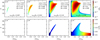 |
Fig. 1. Color coded growth rates γ/Ωe (top panels) and wave frequencies ω/Ωe (bottom panels) for cases 1.a, 1.b, 1.c, and 1.d (from left to right). |
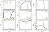 |
Fig. 2. Wave-number dispersion for the fastest-growing unstable modes (with maximum growth rates) in case 1.c, corresponding to different angles of propagation (θ) and different ranges of unstable wave-numbers: BEFI at θ = 65° (black), oblique HFI at θ = 45° (green), and FHFI at θ = 0° (orange). Top panels: wave frequency (left), growth rates (center), and polarization (right). Middle panels: longitudinal and transverse components of the wave electric components. Bottom panels: cartesian components of the wave magnetic field. See further details in the text. |
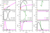 |
Fig. 3. Wave-number dispersion for the fastest growing unstable modes (with maximum growth rates) in case 1.d, corresponding to different angles of propagation (θ) and different ranges of unstable wave-numbers: BEFI at θ = 68° (black), oblique HFI at θ = 40° (green), beaming ESI at θ = 0° (purple), and FHFI at θ = 0° (orange). Top panels: wave frequency (left), growth rates (center), and polarization (right). Middle panels: longitudinal and transverse components of the wave electric components. Bottom panels: cartesian components of the wave magnetic field. See further details in the text. |
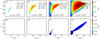 |
Fig. 4. Color coded growth rates γ/Ωe (top panels) and wave frequencies ω/Ωe (bottom panels) for cases 2.a, 2.b, 2.c and 2.d, from left to right. |
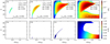 |
Fig. 5. Color coded growth rates γ/Ωe (top panels) and wave frequencies ω/Ωe (bottom panels) for cases 3.a, 3.b, 3.c and 3.d, from left to right. |
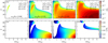 |
Fig. 6. Color coded growth rates γ/Ωe (top panels) and wave frequencies ω/Ωe (bottom panels) for cases 4.a, 4.b, 4.c and 4.d, from left to right. |
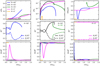 |
Fig. 7. Wave-number dispersion for the fastest-growing unstable modes (with maximum growth rates) in case 4.c, corresponding to different angles of propagation (θ) and different ranges of unstable wave-numbers: BEFI at θ = 63° (black), oblique HFI-1 at θ = 55° (green), oblique HFI-2 at θ = 83° (blue), beaming ESI at θ = 0° (purple), and FHFI at θ = 0° (orange). Top panels: wave frequency (left), growth rates (center), and polarization (right). Middle panels: longitudinal and transverse components of the wave electric components. Bottom panels: cartesian components of the wave magnetic field. See further details in the text. |
Figure 1 presents the four subcases of case 1, where thermal velocities of the beaming and background populations are comparable αb/c ≃ α0/c = 0.07, and are only slightly higher than beaming speed Ub/c = 0.065. The unstable spectra show the wave number (ck/ωpe) dispersion of the growth rate (γ/Ωe, upper panels) and the wave frequency (ωr/Ωe, lower panels) as functions of the propagation angle (θ). Both the growth rate and wave frequency are color coded on the right side of the respective panels. Very low growth rates of BEFI are obtained in case 1.a (left panels), with for example a maximum γmax/Ωe = 0.007 when background electrons have a major density n0/ne = 0.6 > nb/ne = 0.2. With decreasing density contrast between background and beaming electrons, the peak growth rate of BEFI increases by one order of magnitude for case 1.b, that is, for n0/ne = 0.5 and nb/ne = 0.25, and may reach γmax/Ωe ≃ 0.21 for case 1.d, for even more dense electron beams with nb/ne = 0.45 > n0/ne = 0.1. The results for case 1.d are indeed very similar to those obtained by López et al. (2020b) in the absence of background electrons. The comparison of the four cases shows a clear and significant inhibition of BEFI under the influence of background electrons. This instability remains aperiodic (ωr = 0) for all these plasma configurations, which is a specific feature that may help to differentiate from other unstable modes.
In the unstable spectra for cases 1.c and 1.d, we can also distinguish other modes of different nature, in general with finite wave frequency ωr ≠ 0, but with (maximum) growth rates much lower than those of BEFI. A distinction can still be made between these two spectra. Thus, in the panels for case 1.c, at small quasi-parallel angles θ < 20° and small wave-numbers, we may identify the firehose heat-flux instability (FHFI), and for more oblique angles and larger wave-numbers the oblique branches of heat-flux instabilities, which may combine FHFI and whistler heat-flux (WHF) instabilities, which are discussed in more detail in López et al. (2019a); see for example their Fig. 3. These heat-flux instabilities are triggered by an effective anisotropy in velocity space, as resulting from the asymmetry in the thermal spread of the beaming and background populations. These instabilities may therefore not be very sensitive to the variation of (relative) number density. For the denser counter-beams in case 1.d, the electrostatic beaming instabilities (i.e., with a major longitudinal electric field component EL = E ⋅ k) are also predicted at parallel and small θ propagation. In this case, the quasi-parallel unstable spectrum is already complex, showing a superposition of unstable modes with finite frequency, increasing with the wave number. However, the maximum growth rates of all the other unstable modes remain much lower than those of BEFI. Clearly, in all these cases, BEFI is not in competition with other instabilities, and is predicted to operate as the only radiative mechanism, with possible consequences on the relaxation of electron counter-beams. The corresponding plasma beta parameters, β0 and βb, as shown in Table 1, take comparable values around or slightly lower than 1, which means conditions near the equipartition of kinetic and magnetic energy specific to the solar wind in for example CIRs and terrestrial bow shock.
Aiming to decipher the nature of the unstable modes, in Fig. 2 we describe the main properties of the fastest growing modes, that is, those with maximum growth rates, corresponding to each instability in case 1.c from Fig. 1. The upper panels of Fig. 2 show the wave frequency (left), growth rate (middle), and polarization (right) defined as P = Sign(ωr)Re{i(Ex/Ey)}. This polarization is relevant to the electromagnetic modes, circular (or elliptically) polarized, with P > 0 meaning right-handed (RH) polarization and P < 0 left-handed (LH) polarization. The maximum growth rate (γmax/Ωe = 0.208), which is associated with the fastest growing mode, is obtained for BEFI at θ ≃ 65° (black lines), as an aperiodic mode (ωr = 0) purely growing in time. The lower panels in the middle row show components of the wave electric field, longitudinal (or parallel) and transverse to the direction of propagation (i.e., to k), for three distinct modes: BEFI with maximum growth rate at θ = 65° (black lines in the left panel); the oblique branch of the HFIs, in this case, firehose-like modes, LH-polarized (P < 0), and with maximum growth rate at θ = 45° (green lines in the middle panel); and for parallel propagation (θ = 0) a FHFI, circularly LH-polarized with P = −1 < 0 and only a transverse component (ET) of the wave electric field (orange lines in the right panel). Shown in the bottom panels are the corresponding cartesian components of the wave magnetic fields, which confirm the nature of these modes. We note that for BEFI the major component is By, which is another common feature of the firehose instability driven by the temperature anisotropy of electrons (Camporeale & Burgess 2008).
Figure 3 shows the same details as in Fig. 2, but for the main properties of the fastest growing unstable modes in case 1.d, those corresponding to the peaking growth rates in Fig. 1. In this case, the relative density of the background electrons is only n0/ne = 0.1, and the unstable wave spectra resemble those obtained by López et al. (2020b), for similar plasma parameters but in the absence of background electrons. For BEFI (black lines), the value of maximum grow rate is higher, and is obtained at θ ≃ 68°. The maximum growth rate of the oblique HFI (green lines) remains lower than that of BEFI, and is obtained at θ ≃ 40°. But in this case, in the oblique HFI, one may observe that FHF (LH-polarized, with P < 0, at lower wave-numbers) couples with WHF (RH-polarized, with P > 0, at higher wave-numbers), as also shown by López et al. (2020a). We also point out the similarity between the properties of these modes and those obtained for an asymmetric electron plasma-beam system (López et al. 2020a). For parallel propagation (θ = 0°), we find not only the FHFI (orange lines), but also the electrostatic (ES) electron beaming instability (EBI, with purple lines). For both of them, maximum growth rates are less than that of BEFI. This oscillatory (ω ≠ 0) beaming mode is most probably excited by the asymmetric counter-drifting beam and background populations of electrons, by contrast to previous studies in the absence of background electrons (López et al. 2020b), where symmetric counter-beams were able to trigger an aperiodic (ω = 0) two-stream instability. This ES mode seems to couple to EM modes, FHF modes with a Bx component at low wave-numbers, and the other oblique, BEFI or WHF modes, with a major By transverse component of the wave magnetic field. This mode (apparently of a hybrid nature) is not of interest in our present analysis, but could be investigated in future studies.
Figure 4 presents the unstable solutions obtained for cases 2.a-d, which are similar to cases 1.a-d, but for a cooler background population, this time with α0/c = 0.04 < αb/c = 0.07. For the same relative densities, as shown in Table 1, profiles of the unstable spectra are similar to those obtained in Fig. 1, showing a dominance of BEFI. The highest peaking (maximum) growth rates are obtained for BEFI, in general, at oblique angles, which increase with decreasing influence of the background electrons (from left to right). The growth rates increase similarly, but their maximum values, indicated in each panel in Fig. 4, are lower than those obtained in Fig. 1, meaning that BEFI is inhibited by a cooler background population of electrons. We also note that unlike case 1.d., the ES instabilities are missing from the unstable spectra of case 2.d, despite the similarity between the plasma configurations.
3.2. From BEFI to ES instabilities: cases 3 and 4
Next let us explore the properties of BEFI for cases 3.a-d, when the electron background population is even cooler, that is, α0/c = 0.02, and for the same set of relative number densities, as shown in Table 1. The unstable solutions are displayed in Fig. 5 as color coded wave frequencies (bottom panels) and growth rates (top panels). In this case, BEFI remains fairly distinct and dominant, with growth rates higher (or even much higher) than in all the other modes predicted by the linear theory. The inhibiting effect of a cooler electron background is confirmed by for example the maximum growth rates, which are indicated in each panel, and are lower than those obtained for the corresponding cases in Fig. 4. However, in case 3.d, when the relative density of the background population is very low, that is, n0/ne = 0.1, the growth rates of ES modes with (quasi-)parallel wave-vectors become important; they are still less than those of BEFI, but are already markedly higher than those of ES modes obtained in case 1.d. This is what we can call – as also suggested by López et al. (2020b) and Moya et al. (2022) – the transition from the dominance of BEFI to the regime of ES instabilities, which is specific to much cooler electron populations; see for example Fig. 4 in Moya et al. (2022). Although these electrostatic instabilities are not the object of our study, we can explain these results by mentioning that, in the velocity distributions (not shown here), case 3.d shows peaks of the counter-beams and corresponding slopes (δfb/δv ∝ γ > 0) that are more prominent than those for case 1.d. In case 2.d (and also case 1.c), the same peaks and corresponding slopes are much lower, below the threshold of these instabilities.
Figures 6 and 7 show that this transition can be even steeper when the electron beams are cooler than the background population; that is, for cases 4.a–d, when αb = 0.04 < α0 = 0.07. In Fig. 6, growth rates of BEFI (top panels) show the same inhibition under the influence of background electrons, but contrary to that, BEFI only keeps the highest growth rate for a sufficiently dense background population, for instance, in cases 4.a and 4.b. Already in case 4.b, but especially in the other two cases, 4.c and 4.d, the spectra of instabilities become much more complicated due to new unstable solutions, both at oblique propagation angles and in directions parallel and quasi-parallel to the magnetic field. By comparison with BEFI, these new instabilities are oscillatory (or periodic) in time, that is, with ωr ≠ 0; see the bottom panels in Fig. 6. This property helps us to differentiate them, given that their growth rates become comparable to (case 4.c) or even exceed (case 4.d) those of BEFI. We should not forget that the two-stream aperiodic instability predicted in the absence of a background population is expected in this case as well. This instability seems to be identified in case 4.d at low angles and large wave-numbers, as the mode with the highest (maximum) growing rates but with a very small frequency ωr → 0. For a better distinction, but also for a preliminary identification of the nature of the unstable modes, in Fig. 7 we represent the detailed properties of the most unstable modes, which are associated with the maximum growth rates of different modes distinguished in case 4.c (as above in Figs. 2 and 3).
The maximum growth rate of BEFI (black lines) is obtained at θ = 63°, and in this case is comparable with that of ES electron beaming instability (at θ = 0°), which is indicated with purple lines. At oblique angles, this time we can also identify two heat-flow (HF) instabilities with ωr ≠ 0. We already know of the oblique HF found at intermediary oblique angles and larger wave-numbers, which is a WHF with RH polarization and a maximum growth rate at θ = 55°, as indicated with green lines in Fig. 7, as in Fig. 3. A new unstable mode is predicted at very oblique angles (indicated with blue lines in Fig. 7), and combines a firehose HF (FHF) of LH polarization at low wave-numbers with a WHF of RH polarization at large wave-numbers. Even the profile of growth rates shows two humps, corresponding to two different modes. The one obtained at large wave-numbers appears to connect to the WHF mode obtained at lower oblique angles (e.g., for all cases 4.b, 4.c, and 4.d), but nevertheless remains distinct. For both cases 4.c and 4.d, the growth rates of these two modes remain lower than BEFI. The influence of these RH-polarized modes extends to low angles of propagation, becoming visible at sufficiently large wave-numbers and explaining the major magnetic field component By obtained already in case 1.d for the ES mode (purple lines). However, we note that in case 4.d, by far the highest growth rate is that of the aperiodic two-stream instability propagating in a parallel direction, a robust and highly competitive instability of two symmetric, highly dense counter-beams, as described by López et al. (2020b). For the oblique instabilities, the wave-number dispersion of the electric and magnetic field components shows similar profiles, and all resemble those obtained in Fig. 3. By comparison to case 1.d, BEFI already has a significant EL at low wave-numbers, where EL ∼ ET. However, the fastest growing mode, with a maximum growth rate, has the same hybrid nature, with a major EL ≫ ET, and a major By. For θ = 0°, we again find a purely electromagnetic FHF (orange lines) with LH polarization and a growth rate much lower than that of BEFI.
3.3. Maximum growth rates (thresholds) of BEFI
Linear theory can also offer a more comprehensive image of BEFI, if we compute the maximum growth rates and build maps of their contour levels as a function of the main plasma parameters; in this case, the (normalized) beam speed Ub/c, which is the main source of free energy, but also the plasma beta parameter, for example βb for the beam. Figure 8 displays the normalized maximum growth rates, γmax/Ωe, coded according to the color bar on the right side and obtained for BEFI for the situations specific to case 1, when the beam and background electrons have the same thermal spread αb = α0, and three different density ratios nb/ne = 0.15 (left), nb/ne = 0.25 (center), and nb/ne = 0.35 (right). The main features of BEFI are already known, that is, for the same βb the growth rates are significantly enhanced with increasing beam (or drift) speeds. Contour lines (black or white) can be fitted to various mathematical expressions of Ub/c as a function of βb (see e.g., Shaaban et al. 2018b; Moya et al. 2022) in order to quantify the beam speed thresholds of this instability, though here we limit ourselves to a qualitative analysis.
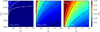 |
Fig. 8. Maximum growth rates γmax/Ωe (color coded) obtained for BEFI for α0 = αb (cases 1), and different density ratios nb/ne = 0.15 (left), nb/ne = 0.25 (center), and nb/ne = 0.35 (right). Levels above contours at γmax/Ωe = 0.3 correspond to the ESI (middle and right panels). |
The effect of background electrons also becomes obvious if we compare with the maximum growth rates of BEFI obtained in López et al. (2020b) for n0/ne = 0, which are markedly higher than those derived here; see for example those in the right panel for the same beam velocities and the same plasma beta. Moreover, the three panels in Fig. 8 show a uniform effect of the background population, which tends to suppress the instability, markedly inhibiting (from right to left) the maximum growth rates, and increasing the instability thresholds; see for example the contours at γmax/Ωe = 0.06 and 0.1 in the middle and right panels. In the middle panel, for a relative density of the beam of nb/ne = 0.25, and n0/ne = 0.5 for the background, one can observe that BEFI can still be triggered with a reasonable maximum growth rate γmax/Ωe ≃ [0.10 − 0.15], if the beta parameter and beam speed are sufficiently high2, that is, βb > 0.2 and Ub/c > 0.065, respectively. If the background electrons are dominant, for example, with a relative density n0/ne = 0.7, as in the left panel, BEFI can barely be excited, with very low growth rates γmax/Ωe ≃ 10−3 approaching and describing the plasma conditions of marginal stability (γ → 0) against BEFI. With a decreasing presence of background electrons, the beam speed characteristic of marginal stability is also markedly lowered, as already found for the instability thresholds. On the other hand, in the middle and right panels, above the contour level around γmax/Ωe ≃ 0.3 we can identify the regime of ESI, the maximum growth rates of which become far superior to BEFI.
The shape of these thresholds is very similar to that obtained for the thresholds of FHFI induced in the direction parallel to the magnetic field by a single (asymmetric) strahl or beam in the solar wind (Shaaban et al. 2018a,b). By virtue of these properties, we can treat BEFI as an instability triggered by a double heat flux. But moreover, BEFI is from the category of the oblique heat-flux instabilities that propagate or develop in highly oblique directions with respect to the magnetic field, as the oblique WHF instability (Verscharen et al. 2019; López et al. 2020a). In contrast to the parallel heat-flux instabilities, the oblique ones can effectively contribute to the relaxation of the electron beams through an efficient resonant scattering of beaming electrons (and do not require that the electrons and waves counter-propagate), as shown not only in numerical simulations (Micera et al. 2020; Vo et al. 2022) but also in a series of recent observations (Cattell et al. 2020). Therefore, we expect BEFI-like instabilities to play an effective role in the relaxation of double electron strahls or beams, that is, those counter-beams with a sufficiently high thermal spread, as predicted by their linear proprieties, as discussed in this section. This could be the case for the electron counter-beams observed in CIRs, but also in the interplanetary shocks and CME foreshocks at sufficiently large heliocentric distances (e.g., 1 AU and beyond). However, we must mention that the observed electron counter-beams are not necessarily symmetrical; where they are asymmetrical, the oblique instability can change its properties, becoming periodic (ωr ≠ 0) and possibly whistler-like in nature.
4. PIC simulations
In order to validate the predictions from linear theory examined in Sect. 3, here we present results from simulations that also describe the evolution of BEFI in time. We used a 2D explicit PIC code based on the KEMPO1 code from Matsumoto & Omura (1993). Our simulation domain is composed of 512 × 512 grid cells, with Lx = Ly = 153.6 cωpe and 625 particles per grid per species. The mass ratio is mp/me = 1836, the plasma to gyro-frequency ωpe/Ωce = 20, the time step is Δt = 0.01/ωpe, and the simulation runs until tmax = 2000/ωpe. We chose to present the simulation results for four cases, 1.c, 1.d, 3.d, and 4.d, which confirm the excitation of BEFI for different plasma conditions, but also allow us to compare the wave fluctuations triggered by different initial conditions; that is either for different relative densities of the electron beams, if we compare cases 1.c and 1.d, or for different thermal speeds of the electron populations, contrasting cases 1.d and 3.d, or 1.c and 4.d.
Figure 9 displays the evolution in time of the fluctuating magnetic field energy density  and the electric energy density
  for the time interval of the simulations. From the figure, we can see that cases 1.c, 1.d, and 3.d (all cases initially satisfying Ub ≲ αb) are qualitatively similar. In all three cases, in agreement with linear theory predictions, the fastest developing BEFI (i.e., with maximum growth rate) has a hybrid nature, with an electric field component (mainly contributing to WE) that grows at the beginning faster than the electromagnetic (EM) transverse component (WB). However, as time advances, the EM energy density WB arises and reaches levels of about one order of magnitude larger than the electric energy density WE. For cases 3.d and 4.d, the increasing slopes of WB are indeed higher than case 1.d, as predicted by the maximum growth rates (γmax) obtained from linear theory3.
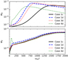 |
Fig. 9. Temporal evolution of the magnetic (top) and electric (bottom) field energy for cases 1.c, 1.d, 3.d, and 4.d. |
The growth of BEFI fluctuations in time is confirmed in Fig. 10 by the FFT spectra of the normalized energy density |FFT(δB/B0)|2, computed for the out-of-plane (perpendicular) component of the fluctuating magnetic field. The levels of fluctuations are coded in the right-hand color bars. Displayed are four time snapshots up to (or near) the saturation,, for the same cases 1.c, 1.d, 3.d, and 4.d, from top to bottom, respectively. The 2D dispersion at large propagation angles in the wave-vector space (k∥, k⊥) resemble those from linear theory, especially at early moments in time, when BEFI fluctuations do not yet reach very high amplitudes (intensities) where they are affected by nonlinear decays. Additional spots that are visible later in time at different propagation angles may indeed signify fluctuations of daughter waves generated nonlinearly via three- or four-wave nonlinear decays. These results are very similar to those from Fig. 5 in López et al. (2020b), which were obtained for BEFI in the case with no electron background. However, BEFI fluctuations are visibly inhibited by the presence of background electrons. In this sense, the contrast between the levels of fluctuation in Fig. 10 is also very relevant, such as that between the levels of fluctuation obtained for the same time snapshots in cases 1.c and 1.d.
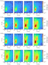 |
Fig. 10. Time snapshots of the FFT (normalized) energy density computed for the out-of-plane (perpendicular) component of the magnetic field for cases 1.c, 1.d, 3.d, and 4.d. |
In case 4.d (with Ub > αb), our BEFI is predicted by linear theory in close competition with the ES instabilities (see also the results presented in Figs. 9–11 in López et al. 2020b, where the initial conditions also entail beam speeds higher than thermal speeds, but in the absence of an electron background). Indeed, the green dotted line in Fig. 9 shows a quick increase and relaxation of the fluctuating electric energy density WE, with a narrow and relatively small peak followed by a drop and then a more robust growth of the magnetic energy density WB due to BEFI. In this case, the ES instability is excited first (at much lower timescales), as already indicated in Fig. 9. BEFI develops as a secondary but more robust instability, and this is also confirmed in the last row of Fig. 10 for the same timescales of BEFI in cases 1.c, 1.d, and 3.d. However, for case 4.d, the oblique maxima of BEFI are more disperse or less compact, most probably due to linear or nonlinear interactions with fluctuations of another nature. The earlier ES excitations propagating at small angles with respect to the magnetic field are confirmed in Fig. 11, where we display earlier time snapshots of the FFT (normalized) energy density for the parallel electric field component in case 4.d. The levels of fluctuation are color coded in the right-hand bars, and reach a maximum (saturation) at about ωpet = 61.44, much earlier than the first time snapshot shown in Fig. 10.
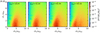 |
Fig. 11. Time snapshots of the FFT (normalized) energy density computed for the parallel electric field component in case 4.d, showing an early time fast growth and saturation of ES instability. |
5. Conclusions
As space plasmas are weakly collisional (or even noncollisional), we expect wave instabilities to have multiple implications, especially in that they may facilitate the conversion of free energy of plasma particles, as well as energy transfer between species. López et al. (2020b) and Moya et al. (2022) recently showed that two symmetric electron counter-beams aligned to the guiding magnetic field can induce an EM firehose-like instability, aperiodic and propagating highly obliquely to the magnetic field. In the present work, we investigate this instability under typical conditions found in the heliosphere, calling it the beaming electron firehose instability (BEFI). We assume a specific parameterization of the plasma system, including a background embedding plasma of electrons and ions (protons). Counter-beaming electrons penetrating the background solar wind are often reported by in situ observations, in various contexts such as interplanetary shocks, CIRs, and closed magnetic field topology specific to CMEs.
Here, we rely on such observations to define the plasma model introduced in Sect. 2, and to identify the conditions found favorable to BEFI; see parametric cases in Table 1. In Sect. 3, we describe the linear spectra of unstable waves for the selected cases in Table 1, varying the relative densities and thermal speeds of the electron components. Particularly relevant for BEFI are the regimes identified in Figs. 1–5 for cases 1.a–d, 2.a–d, and 3.a–c, when either BEFI alone is predicted, or has a (maximum) growth rate much higher than all the other instabilities in the spectra. The influence of the background population can be quantified in terms of relative density and thermal spread. For the cases studied here, BEFI growth rates are significantly reduced if relative beam densities are less than 20% of the total density (implying background electrons with relative density exceeding 80%), making the existence of this instability critical. For a slightly cooler background population – compare for instance cases 1 and 2 –, the range of unstable wave-numbers increases. A similar effect is obtained in case 3 for a slightly cooler beam. However, for even lower thermal speeds or higher densities of the beams, as in case 4, the (maximum) growth rates become dominated by the ES instabilities at lower angles of propagation, as already shown in López et al. (2020b) and Moya et al. (2022).
The linear properties of dispersion and stability, including the instability thresholds, lead us to the conclusion that BEFI is analogous to heat-flux instabilities generated by unidirectional electron strahls or beams in the solar wind. However, BEFI is triggered by the double heat flux of the counter-beams (or double strahl) of electrons, but for sufficiently low beaming speeds (or associated heat fluxes) in the range of the thermal speed of electron beams. However, in the present analysis with two electron counter-beams and background populations, the configuration of linear spectra of unstable modes becomes much more complicated. In addition to the ES instabilities (for higher beaming speeds), we also identify periodic instabilities (with ωr ≠ 0) that do not appear in the absence of the background electron population when only symmetric counter-beams are present (López et al. 2020b). These unstable wave modes are specific to asymmetric electron beam-plasma configurations, which here result from the combination of each electron beam with the background population. More details can be found in a recent parametric analysis of electron heat-flux instabilities in the solar wind conditions (López et al. 2020a). Future works should also investigate more complex plasma systems with asymmetric counter-beams embedded with background electrons, for which we expect BEFI to become a periodic mode as well; see for instance the case in Fig. 7 in López et al. (2020b). In such a case, BEFI will probably blend more easily with other modes and make them difficult to distinguish. From the analogy with the heat-flux instabilities, BEFI compares better with the oblique whistlers, which can contribute to the scattering and relaxation of unidirectional strahls in the solar wind (Micera et al. 2020; Cattell et al. 2020).
PIC simulations confirm the results of the linear kinetic theory (Sect. 4), not only for the conditions in which the BEFI is predicted to be the primary excitation, with major growth rates, but also when it develops as a secondary instability. We tested the cases associated with high growth rates in the PIC simulations in order to reduce the computational time and obtain results of increased confidence. The BEFI fluctuations develop (aperiodically) at highly oblique propagation angles to the magnetic field, in agreement with the wave-number and angular dispersion of the (initial) linear growth rates. Moreover, the levels reached by these fluctuations are diminished with the increasing presence of background electrons, which is also in contrast to the results in López et al. (2020b) obtained in the absence of background electrons. In the regimes of competition with ES instabilities, BEFI still develops as a secondary but sufficiently robust instability to produce intense EM fluctuations, which are long-lasting up until their saturation. Therefore, we can expect BEFI to be involved in the regulation of electron counter-beams with properties similar to those investigated here. The findings that we present here should motivate future theoretical and observational studies modeling the evolution of such double electron strahls or beams under the consistent action of BEFI-like fluctuations, and comparison with in situ observations in space plasmas would offer further insight.
For a more fluid-like regime of electron (counter-)beams, the instability wave spectra are dominated by the ES fluctuations (with the highest growth rates), while the EM or hybrid fluctuations may be predicted either for low drifts, i.e., vd < αe, or for very high, relativistic beaming speeds corresponding to more than 100 keV (Gary & Nishimura 2003; Lazar et al. 2009; Bret 2009; Jao & Hau 2016).
Acknowledgments
The authors acknowledge support from the Ruhr-University Bochum and the Katholieke Universiteit Leuven, and Mansoura University. These results were also obtained in the framework of the projects C14/19/089 (C1 project Internal Funds KU Leuven), G.0D07.19N (FWO-Vlaanderen), SIDC Data Exploitation (ESA Prodex-12), Belspo project B2/191/P1/SWiM, and Fondecyt No. 1191351 (ANID, Chile). P.S. Moya is grateful for the support of KU Leuven BOF Network Fellowship NF/19/001 and ANID Chile through FONDECyT grant No. 119135. R.A.L. acknowledges the support of ANID Chile through FONDECyT grant No. 11201048. Powered@NLHPC: This research was partially supported by the supercomputing infrastructure of the NLHPC (ECM-02). We thank the anonymous reviewer for a careful reading of our paper, as well as for the pertinent observations.
References
- Anderson, B. R., Skoug, R. M., Steinberg, J. T., & McComas, D. J. 2012, J. Geophys. Res.: Space Phys., 117, A04107 [NASA ADS] [Google Scholar]
- Bame, S. J., Asbridge, J. R., Feldman, W. C., Gosling, J. T., & Zwickl, R. D. 1981, Geophys. Res. Lett., 8, 173 [NASA ADS] [CrossRef] [Google Scholar]
- Beck, R. 2015, A&ARv, 24, 4 [Google Scholar]
- Berčič, L., Maksimović, M., Landi, S., & Matteini, L. 2019, MNRAS, 486, 3404 [Google Scholar]
- Bret, A. 2009, ApJ, 699, 990 [NASA ADS] [CrossRef] [Google Scholar]
- Camporeale, E., & Burgess, D. 2008, J. Geophys. Res.: Space Phys., 113, A07107 [NASA ADS] [Google Scholar]
- Carcaboso, F., Gómez-Herrero, R., Espinosa Lara, F., et al. 2020, A&A, 635, A79 [NASA ADS] [CrossRef] [EDP Sciences] [Google Scholar]
- Cattell, C. A., Short, B., Breneman, A. W., & Grul, P. 2020, ApJ, 897, 126 [Google Scholar]
- Che, H., Goldstein, M. L., Salem, C. S., & Viñas, A. F. 2019, ApJ, 883, 151 [NASA ADS] [CrossRef] [Google Scholar]
- Cremades, H., Iglesias, F. A., St. Cyr, O. C., et al. 2015, Sol. Phys., 290, 2455 [NASA ADS] [CrossRef] [Google Scholar]
- Fitzenreiter, R. J., Ogilvie, K. W., Bale, S. D., & Viñas, A. F. 2003, J. Geophys. Res.: Space Phys., 108, 1415 [NASA ADS] [CrossRef] [Google Scholar]
- Fried, B. D., & Conte, S. D. 1961, The Plasma Dispersion Function (New York: Academic Press) [Google Scholar]
- Ganse, U., Kilian, P., Vainio, R., & Spanier, F. 2012, Sol. Phys., 280, 551 [NASA ADS] [CrossRef] [Google Scholar]
- Gary, S. P., & Nishimura, K. 2003, Phys. Plasmas, 10, 3571 [NASA ADS] [CrossRef] [Google Scholar]
- Gosling, J. T., Baker, D. N., Bame, S. J., et al. 1987, J. Geophys. Res., 92, 8519 [Google Scholar]
- Hammond, C. M., Feldman, W. C., McComas, D. J., Phillips, J. L., & Forsyth, R. J. 1996, A&A, 316, 350 [Google Scholar]
- Jao, C. S., & Hau, L. N. 2016, Phys. Plasmas, 23, 112110 [NASA ADS] [CrossRef] [Google Scholar]
- Kajdič, P., Blanco-Cano, X., Opitz, A., et al. 2013, AIP Conf. Ser., 1539, 203 [Google Scholar]
- Larson, D. E., Lin, R. P., McFadden, J. P., et al. 1996, Geophys. Res. Lett., 23, 2203 [NASA ADS] [CrossRef] [Google Scholar]
- Lavraud, B., Opitz, A., Gosling, J. T., et al. 2010, Annal. Geophys., 28, 233 [NASA ADS] [CrossRef] [Google Scholar]
- Lazar, M., Schlickeiser, R., Wielebinski, R., & Poedts, S. 2009, ApJ, 693, 1133 [NASA ADS] [CrossRef] [Google Scholar]
- Lazar, M., Pomoell, J., Poedts, S., Dumitrache, C., & Popescu, N. A. 2014, Sol. Phys., 289, 4239 [NASA ADS] [CrossRef] [Google Scholar]
- Lee, S.-Y., Ziebell, L. F., Yoon, P. H., Gaelzer, R., & Lee, E. S. 2019, ApJ, 871, 74 [NASA ADS] [CrossRef] [Google Scholar]
- Li, X., & Habbal, S. R. 2000, J. Geophys. Res.: Space Phys., 105, 27377 [NASA ADS] [CrossRef] [Google Scholar]
- López, R. A., Lazar, M., Shaaban, S. M., et al. 2019a, ApJ, 873, L20 [CrossRef] [Google Scholar]
- López, R. A., Shaaban, S. M., Lazar, M., et al. 2019b, ApJ, 882, L8 [Google Scholar]
- López, R. A., Lazar, M., Shaaban, S. M., Poedts, S., & Moya, P. S. 2020a, ApJ, 900, L25 [Google Scholar]
- López, R. A., Lazar, M., Shaaban, S. M., Poedts, S., & Moya, P. S. 2020b, Plasma Phys. Control. Fusion, 62, 075006 [Google Scholar]
- López, R. A., Shaaban, S., & Lazar, M. 2021, J. Plasma Phys., 87, 905870310 [CrossRef] [Google Scholar]
- Macneil, A. R., Owens, M. J., Lockwood, M., Štverák, Š., & Owen, C. J. 2020, Sol. Phys., 295, 16 [Google Scholar]
- Maksimovic, M., Zouganelis, I., Chaufray, J. Y., et al. 2005, J. Geophys. Res.: Space Phys., 110, A09104 [NASA ADS] [CrossRef] [Google Scholar]
- Matsumoto, H., & Omura, Y. 1993, Computer Space Plasma Physics: Simulation Techniques and Software (Tokyo: Terra Scientific Publishing Company) [Google Scholar]
- Micera, A., Zhukov, A. N., López, R. A., et al. 2020, ApJ, 903, L23 [NASA ADS] [CrossRef] [Google Scholar]
- Montgomery, M. D., Asbridge, J. R., Bame, S. J., & Feldman, W. C. 1974, J. Geophys. Res., 79, 3103 [NASA ADS] [CrossRef] [Google Scholar]
- Moya, P. S., López, R. A., Lazar, M., Poedts, S., & Shaaban, S. M. 2022, ApJ, 937, 49 [NASA ADS] [CrossRef] [Google Scholar]
- Nieves-Chinchilla, T., & Viñas, A. F. 2008, J. Geophys. Res.: Space Phys., 113, A02105 [Google Scholar]
- Pick, M., & Vilmer, N. 2008, A&ARv, 16, 1 [NASA ADS] [CrossRef] [Google Scholar]
- Pilipp, W. G., Miggenrieder, H., Montgomery, M. D., et al. 1987, J. Geophys. Res., 92, 1093 [NASA ADS] [CrossRef] [Google Scholar]
- Pulupa, M., & Bale, S. D. 2008, ApJ, 676, 1330 [NASA ADS] [CrossRef] [Google Scholar]
- Schlickeiser, R. 2005, Plasma Phys. Control. Fusion, 47, A205 [Google Scholar]
- Schlickeiser, R., Krakau, S., & Supsar, M. 2013, ApJ, 777, 49 [NASA ADS] [CrossRef] [Google Scholar]
- Shaaban, S. M., Lazar, M., & Poedts, S. 2018a, MNRAS, 480, 310 [Google Scholar]
- Shaaban, S. M., Lazar, M., Yoon, P. H., & Poedts, S. 2018b, Phys. Plasmas, 25, 082105 [NASA ADS] [CrossRef] [Google Scholar]
- Shaaban, S. M., Lazar, M., López, R. A., Fichtner, H., & Poedts, S. 2019, MNRAS, 483, 5642 [NASA ADS] [CrossRef] [Google Scholar]
- Skoug, R. M., Feldman, W. C., Gosling, J. T., McComas, D. J., & Smith, C. W. 2000, J. Geophys. Res., 105, 23069 [NASA ADS] [CrossRef] [Google Scholar]
- Steinberg, J. T., Gosling, J. T., Skoug, R. M., & Wiens, R. C. 2005, J. Geophys. Res.: Space Phys., 110, A06103 [NASA ADS] [CrossRef] [Google Scholar]
- Stix, T. H. 1992, Waves in Plasmas (New York: AIP Press) [Google Scholar]
- Stockem, A., Lerche, I., & Schlickeiser, R. 2007, ApJ, 659, 419 [NASA ADS] [CrossRef] [Google Scholar]
- Verscharen, D., Chandran, B. D. G., Jeong, S.-Y., et al. 2019, ApJ, 886, 136 [Google Scholar]
- Vo, T., Lysak, R., & Cattell, C. 2022, Phys. Plasmas, 29, 012904 [NASA ADS] [CrossRef] [Google Scholar]
Appendix A: Kinetic dispersion formalism
Without loss of generality, we assume cartesian coordinates (x, y, z) with z-axis parallel to the magnetic field B, and with the wave vector k in the (x − z) plane, such that
where ∥, ⊥ are gyrotropic directions with respect to the magnetic field direction. From the Vlasov-Maxwell equations, one can derive the general wave equation (Stix 1992)

and the general dispersion relation for nontrivial (nonzero) plasma modes (far away from the initial perturbation),
![$$ \begin{aligned} \Lambda (\omega , k) \equiv \mathrm{det} [\Lambda _{ij}] = 0, \end{aligned} $$](/articles/aa/full_html/2023/02/aa45163-22/aa45163-22-eq9.gif)
in terms of the electric field of the wave fluctuation E(k, ω) and the dispersion tensor Λ = |Λij|. For gyrotropic distribution functions Fa(v⊥, v∥) of plasma species of the sort a (e.g., a = 0, 1, 2 for the electron populations, and a = p for protons), the components of the dispersion tensor read as follows:
with  , and
, and
where b = k⊥v⊥/Ωa, Jn(b) is the Bessel function with  being its first derivative, i the imaginary unit, and c the speed of light, and for each species of sort a,
  is the plasma frequency, Ωa = qaB0/(mac) the gyrofrequency, qa the charge, ma the mass, and na the number density.
With the three-component distribution function in Eqs. (1) and (2), the elements of the dispersion tensor take the following expressions:
where Λn(x) = In(x)e−x, with In(x) the modified Bessel function, and

where Z(x) is the standard plasma dispersion function for Maxwellian populations (Fried & Conte 1961). Equivalent expressions for the components of the dielectric tensor are also provided in Stix (1992), pp. 258–260.
All Tables
Four cases corresponding to different thermal velocities α0 and αb (in units of c), and for each case another four distinct subcases (a–d) defined by different relative number densities of the electron background n0/ne or beams nb/ne. For all cases Ub/c = 0.065 and βp = 1.96.
All Figures
|
Fig. 1. Color coded growth rates γ/Ωe (top panels) and wave frequencies ω/Ωe (bottom panels) for cases 1.a, 1.b, 1.c, and 1.d (from left to right). |
| In the text | |
|
Fig. 2. Wave-number dispersion for the fastest-growing unstable modes (with maximum growth rates) in case 1.c, corresponding to different angles of propagation (θ) and different ranges of unstable wave-numbers: BEFI at θ = 65° (black), oblique HFI at θ = 45° (green), and FHFI at θ = 0° (orange). Top panels: wave frequency (left), growth rates (center), and polarization (right). Middle panels: longitudinal and transverse components of the wave electric components. Bottom panels: cartesian components of the wave magnetic field. See further details in the text. |
| In the text | |
|
Fig. 3. Wave-number dispersion for the fastest growing unstable modes (with maximum growth rates) in case 1.d, corresponding to different angles of propagation (θ) and different ranges of unstable wave-numbers: BEFI at θ = 68° (black), oblique HFI at θ = 40° (green), beaming ESI at θ = 0° (purple), and FHFI at θ = 0° (orange). Top panels: wave frequency (left), growth rates (center), and polarization (right). Middle panels: longitudinal and transverse components of the wave electric components. Bottom panels: cartesian components of the wave magnetic field. See further details in the text. |
| In the text | |
|
Fig. 4. Color coded growth rates γ/Ωe (top panels) and wave frequencies ω/Ωe (bottom panels) for cases 2.a, 2.b, 2.c and 2.d, from left to right. |
| In the text | |
|
Fig. 5. Color coded growth rates γ/Ωe (top panels) and wave frequencies ω/Ωe (bottom panels) for cases 3.a, 3.b, 3.c and 3.d, from left to right. |
| In the text | |
|
Fig. 6. Color coded growth rates γ/Ωe (top panels) and wave frequencies ω/Ωe (bottom panels) for cases 4.a, 4.b, 4.c and 4.d, from left to right. |
| In the text | |
|
Fig. 7. Wave-number dispersion for the fastest-growing unstable modes (with maximum growth rates) in case 4.c, corresponding to different angles of propagation (θ) and different ranges of unstable wave-numbers: BEFI at θ = 63° (black), oblique HFI-1 at θ = 55° (green), oblique HFI-2 at θ = 83° (blue), beaming ESI at θ = 0° (purple), and FHFI at θ = 0° (orange). Top panels: wave frequency (left), growth rates (center), and polarization (right). Middle panels: longitudinal and transverse components of the wave electric components. Bottom panels: cartesian components of the wave magnetic field. See further details in the text. |
| In the text | |
|
Fig. 8. Maximum growth rates γmax/Ωe (color coded) obtained for BEFI for α0 = αb (cases 1), and different density ratios nb/ne = 0.15 (left), nb/ne = 0.25 (center), and nb/ne = 0.35 (right). Levels above contours at γmax/Ωe = 0.3 correspond to the ESI (middle and right panels). |
| In the text | |
|
Fig. 9. Temporal evolution of the magnetic (top) and electric (bottom) field energy for cases 1.c, 1.d, 3.d, and 4.d. |
| In the text | |
|
Fig. 10. Time snapshots of the FFT (normalized) energy density computed for the out-of-plane (perpendicular) component of the magnetic field for cases 1.c, 1.d, 3.d, and 4.d. |
| In the text | |
|
Fig. 11. Time snapshots of the FFT (normalized) energy density computed for the parallel electric field component in case 4.d, showing an early time fast growth and saturation of ES instability. |
| In the text | |
Current usage metrics show cumulative count of Article Views (full-text article views including HTML views, PDF and ePub downloads, according to the available data) and Abstracts Views on Vision4Press platform.
Data correspond to usage on the plateform after 2015. The current usage metrics is available 48-96 hours after online publication and is updated daily on week days.
Initial download of the metrics may take a while.