| Issue |
A&A
Volume 673, May 2023
|
|
|---|---|---|
| Article Number | A67 | |
| Number of page(s) | 18 | |
| Section | Extragalactic astronomy | |
| DOI | https://doi.org/10.1051/0004-6361/202244875 | |
| Published online | 08 May 2023 | |
Comparing the host galaxy ages of X-ray selected AGN in COSMOS
Obscured AGN are associated with older galaxies
1
Institute for Astronomy Astrophysics Space Applications and Remote Sensing (IAASARS), National Observatory of Athens, I. Metaxa & V. Pavlou, Penteli 15236, Greece
e-mail: ig@noa.gr
2
Instituto de Fisica de Cantabria (CSIC-Universidad de Cantabria), Avenida de los Castros, 39005 Santander, Spain
3
Sterrenkundig Observatorium, Universiteit Gent, Krijgslaan 281 S9, 9000 Gent, Belgium
4
Max-Planck Institut für Astronomie Königstuhl, 69117 Heidelberg, Germany
5
INAF – Osservatorio di Astrofisica e Scienza dello Spazio di Bologna, Via Piero Gobetti, 93/3, 40129 Bologna, Italy
6
Department of Physics and Astronomy, Clemson University, Kinard Lab of Physics, Clemson, SC 29634, USA
Received:
3
September
2022
Accepted:
25
January
2023
We explore the properties of the host galaxies of X-ray selected AGN in the COSMOS field using the Chandra Legacy sample and the LEGA-C survey VLT optical spectra. Our main goal is to compare the relative ages of the host galaxies of the obscured and unobscured AGN by means of the calcium break Dn(4000) and the Hδ Balmer line. The host galaxy ages are examined in conjunction with other properties such as the galaxy stellar mass, and star-formation rate as well as the AGN Eddington ratio. Our sample consists of 50 unobscured or mildly obscured (NH < 1023 cm−2) and 23 heavily obscured AGN (NH > 1023 cm−2) in the redshift range z = 0.6 − 1. We take specific caution to create control samples in order to match the exact luminosity and redshift distributions for the obscured and unobscured AGN. The majority of unobscured AGN appear to live in young galaxies in contrast to the obscured AGN which appear to live in galaxies located between the young and old galaxy populations. This finding may be in contrast to those evolutionary AGN unification models which postulate that the AGN begin their life in a heavy obscuration phase. The host galaxies of the obscured AGN have significantly lower levels of specific star-formation. At the same time the obscured AGN have lower Eddington ratios indicating a link between the star-formation and the black hole accretion. We find that the distribution of the stellar masses of the host galaxies of obscured AGN is skewed towards higher stellar masses in agreement with previous findings. Our results on the relative age of obscured AGN are valid when we match our obscured and unobscured AGN samples according to the stellar mass of their host galaxies. All the above results become less conspicuous when a lower column density (log NH(cm−2) = 21.5 or 22) is used to separate the obscured and unobscured AGN populations.
Key words: galaxies: nuclei / quasars: supermassive black holes / X-rays: galaxies / galaxies: active
© The Authors 2023
 Open Access article, published by EDP Sciences, under the terms of the Creative Commons Attribution License (https://creativecommons.org/licenses/by/4.0), which permits unrestricted use, distribution, and reproduction in any medium, provided the original work is properly cited.
This article is published in open access under the Subscribe to Open model. Subscribe to A&A to support open access publication.
1. Introduction
Active Galactic Nuclei (AGNs) are among the most luminous sources in the Universe. They are powered by accretion onto supermassive black holes (SMBHs) in their centres (Lynden-Bell 1969). Despite the difference in physical scale between the SMBH and the galaxy spheroid (about nine orders of magnitude), there is a tight correlation between the masses of the SMBH and the galaxy bulge (Silk & Rees 1998; Magorrian et al. 1998; Ferrarese & Merritt 2000; Gebhardt et al. 2000). The physical mechanisms that underlie this correlation are not properly understood but most theoretical models for galaxy evolution predict a regulating mechanism between the AGN power and the star-formation of the host galaxy. The models that explain the AGN and galaxy co-evolution on the basis of mergers (e.g., Hopkins et al. 2008) suggest that when the AGN becomes active it passes a long period in an obscured phase. The obscuring material feeds the AGN that eventually becomes powerful enough to push away the surrounding material and become unobscured (e.g., Ciotti & Ostriker 1997; Hopkins et al. 2006; Hopkins & Hernquist 2006; Somerville & Hopkins 2008; Blecha et al. 2018). Then the unobscured AGN passes a phase of coeval growth where the SMBH accretes material at high Eddington rates and at the same time this stimulates intense star-formation in the centre of the host galaxy (Di Matteo et al. 2005; Hopkins et al. 2008; Zubovas et al. 2013). These are the evolutionary unification models which are differentiated from the standard unification models. The latter postulate that the obscuration in an AGN depends only on the inclination angle relative to the line of sight (Antonucci 1993). A number of observational works provide evidence in support of the above evolutionary scenarios (e.g., Koss et al. 2018; Glikman et al. 2018; Banerji et al. 2021; Hatcher et al. 2021; Mountrichas & Shankar 2023).
In the past years there has been a number of works which examined the validity of the AGN/galaxy co-evolution models. The most widely applied method to study the AGN-galaxy co-evolution is via examining the correlation of the SMBH activity and the star formation rate (SFR) of the host galaxy (e.g., Rovilos et al. 2012; Rosario et al. 2012; Chen et al. 2013; Hickox et al. 2014; Stanley et al. 2015, 2017; Rodighiero et al. 2015; Aird et al. 2012, 2019; Lanzuisi et al. 2017; Harrison et al. 2018; Brown et al. 2019). In many of the above studies the star-formation is measured at far infrared wavelengths from the cold dust emission heated by young stars using data from the Herschel mission. The X-ray luminosity is used as a very good proxy of the AGN power. More recent works attempt to disentangle the effect of the host galaxy on the star-formation by taking into account the position of the host galaxy on the star-formation main sequence as defined by its redshift and stellar mass. These works (Mullaney et al. 2015; Bernhard et al. 2019; Masoura et al. 2018, 2021; Florez et al. 2020; Mountrichas et al. 2021a; Torbaniuk et al. 2021) find again a correlation between the normalised SFR (SFRNORM) and the AGN X-ray luminosity; SFRNORM is defined as the observed SFR divided by the mean SFR of normal galaxies at the same redshift and stellar mass. However, it is not entirely clear whether the correlation between SFR and X-ray luminosity hides an underlying correlation with the galaxy’s stellar mass (Fornasini et al. 2020; Mountrichas et al. 2022c). This would suggest that the AGN power and the SFR evolve in a similar manner because they are fed by the same molecular gas depot of the host galaxy. Some of the above works examined the SFR separately for type-1 and type-2 AGN. They concluded that there is no concrete evidence that the SFR properties differ in the two types of AGN (Masoura et al. 2021; Mountrichas et al. 2021a). Nevertheless, Chen et al. (2015) by analysing a sample of mid-IR selected AGN in the Bootes region, find that the SFR in type-2 AGN is a factor of two higher compared to type-1 AGN.
Additional evidence in support of the evolutionary unification scenarios may come from the comparison of the Eddington ratio distribution in obscured and unobscured AGN (Ananna et al. 2022; Schulze et al. 2015; Kelly & Shen 2013; Schulze & Wisotzki 2010). Ananna et al. (2022) studied the Eddington ratios of low redshift AGN in the Neil Gehrels Swift/Burst Alert Telecope (BAT) AGN spectroscopic survey (BASS). They find that the Eddington ratio distribution of obscured AGN is skewed towards low Eddington ratios. This is in favour of a radiation-driven scenario where the radiation pressure regulates the shape of the torus. This means that when the AGN is luminous the torus is pushed away while the obscured AGN are those which have low Eddington ratios. These findings are not in contrast with the evolution unification scenarios where the birth of an AGN is marked by a long phase of obscuration accompanied by low Eddington ratios.
On the other hand, recent results on the masses of obscured and unobscured AGN may be in contrast to the above evolutionary unification scenarios. Zou et al. (2019) examined optically selected narrow and broad line AGN in the COSMOS field, finding that the type-2 systems have significantly higher stellar masses. This result has been corroborated by other optically selected samples (Mountrichas et al. 2021a; Koutoulidis et al. 2022) although the difference in stellar mass is not prominent when the separation between type-1 and type-2 AGN is based on X-ray obscuration. This difference in stellar mass may suggest that type-2 AGN are more massive because they are associated with older systems and had more time to increase their mass because of merging with satellite galaxies. However, more concrete evidence is necessary in order to pin down the age of these AGN and thus to better constrain the models of AGN and galaxy co-evolution. This evidence can be provided by optical spectroscopy. In a pioneering work Kauffmann et al. (2003) examined the properties of the host galaxies of a large number of AGN in redshifts below z = 0.3 from the Sloan Digital Sky Survey. In particular they examined the galaxy ages using the strength of the calcium 4000-Å break as the primary indicator of the age of the stellar population. They examined the stellar ages of narrow-line and broad-line AGN finding no significant difference between the two populations when their luminosity and redshift is taken into account.
The LEGA-C survey provides the opportunity to expand these studies at redshifts z ∼ 0.7 corresponding to a look-back time of 7 Gyr. The LEGA-C survey has observed 4000 galaxies in the COSMOS field using the VIMOS instrument on VLT providing excellent quality spectroscopy and hence accurate measurements of the calcium break and other age indicators such as the Hδ absorption line. In this work, we examine the properties of the Chandra X-ray selected AGN in the COSMOS field combining the LEGA-C optical spectroscopy with spectral energy distribution (SED) fittings performed with the X-CIGALE code. The optica1 spectroscopy provides robust indicators of the age as well as black hole masses while the SED provide the stellar masses and SFR. Our goal is to examine how the properties of obscured and unobscured AGN evolve with stellar age. This may provide constraints on the galaxy/AGN co-evolution models and evolutionary unification models. Throughout the paper, we assume a standard ΛCDM cosmology with Ho = 69.3 km s−1 Mpc−1, Ωm = 0.286.
2. Data
2.1. The LEGA-C survey
The Very Large Telescope VIMOS LEGA-C survey (van der Wel et al. 2021) collects high signal-to-noise, high resolution spectra for thousands of galaxies in the redshift range 0.6–1. This allows to probe stellar populations (ages and metallicities) and stellar kinematics (velocity dispersions) of thousands of galaxies at a look-back time of ∼7 Gyr. This allows to study with unprecedented accuracy the star-formation history of galaxies.
The LEGA-C survey is based on the UltraVISTA catalogue of Muzzin et al. (2013). This catalogue contains 160 070 sources down to K = 23.4 across 1.62 sq. degrees of the COSMOS field (Scoville et al. 2007). The LEGA-C survey creates a parent sample of galaxies with (spectroscopic or photometric) redshifts in the range 0.6 < z < 1 and with Ks magnitudes brighter than a redshift-dependent limit Ks = 20.7 − 7.5log[(1 + z)/1.8]. The final survey footprint covers 1.4255 square degrees, giving a total survey co-moving volume of ∼3.7 × 10⁶ Mpc3 between z = 0.6 and z = 1.0. The VIMOS observations produced 3029 high signal-to-noise spectra of primary targets in the 6300–8800 Å wavelength range with a resolution of R = 2500. Additional targets have been observed at either higher redshifts or at fainter magnitudes in the primary z = 0.6–1 redshift band. The strength of the Balmer absorption lines and the spectral region around the calcium break at 4000 Å provide the most sensitive diagnostics of the stellar population age (e.g., Kauffmann et al. 2003). The determination of the age distribution of stellar populations at a redshift of about 7 Gyr is one of the main products of the survey.
2.2. The COSMOS Chandra Legacy survey
Civano et al. (2016) present a 4.6 Ms Chandra survey that covers 2.2 deg2 of the COSMOS field. The central area has been observed with an exposure time of ≈160 ksec while the remaining area has exposure time of ≈80 ksec. The limiting depths are 2.2 × 10⁻¹⁶, 1.5 × 10⁻¹⁵ erg cm−2 s−1 in the soft (0.5–2 keV), hard (2–10 keV) bands, respectively. The catalogue contains 4016 sources. Lanzuisi et al. (2017) and Marchesi et al. (2016b) provide X-ray spectral fits for all sources with over 30 counts. For the remaining sources hardness ratios are given defined as HR = (H − S)/(H + S) where H and S are the net (background subtracted) count rates in the 2–7 keV and 0.5–2 keV respectively. These provide a good proxy of the intrinsic column density of the source. As most sources have a low number of counts, Civano et al. (2016) used the Bayesian Estimation HR code (Park et al. 2006) which is particularly effective in the low-count regime.
Marchesi et al. (2016a) matched the X-ray sources with optical/infrared counterparts, using the likelihood ratio technique Sutherland & Saunders (1992). 97% of the sources have an optical/IR counterpart. Finally, a cross-match with the COSMOS photometric catalogue produced by the HELP collaboration Shirley et al. (2019) has been performed. HELP includes data from 23 of the premier extragalactic survey fields, imaged by the Herschel Space Observatory which form the Herschel Extragalactic Legacy Project (HELP). The catalogue provides homogeneous and calibrated multi-wavelength data. The cross-match with the HELP catalogue is done using 1 arcsec radius and the optical coordinates of the counterpart of each X-ray source.
3. Sample selection
3.1. Optical spectra
We cross-correlate the LEGA-C DR-3 spectroscopic catalogue (van der Wel et al. 2021) with the coordinates of the optical counterparts of the COSMOS Chandra Legacy sample. We find 173 common sources of which 163 have optical spectra with good signal-to-noise ratio > 3 per pixel (0.6 Å). Out of these only 107 have reliable measurements in both the Hδ and the calcium break Dn spectral region. Kauffmann et al. (2003) have studied the Hδ − Dn diagram for SDSS optically selected AGN. They find that the continuously star-forming galaxies define a sequence from old galaxies having large values of Dn and low values of Hδ moving progressively to young galaxies which have low values of Dn combined with high values of Hδ. Galaxies which experienced recent star-formation bursts present high Hδ values above the main sequence. However, eight of our sources present low values of Dn, placing them in the young galaxy regime, combined with low values of Hδ which are characteristic of old galaxies. The location of these sources on the Hδ − Dn diagram cannot be easily interpreted using the star-formation history models in Kauffmann et al. (2003). Inspection of their optical spectra suggests that the Lick indices may be contaminated by broad emission features. The details of these galaxies are given in Table 1. These eight sources lie outside the 99% contours of the LEGA-C galaxy population (see the top left panel in Fig. 4). A further eight sources have been discarded because of poor quality spectral energy distribution fits having χ2 > 5, see Sect. 4.1 for details.
Excluded sources lying well below the main Hδ − Dn sequence.
3.2. Photometry
In our analysis, we need reliable estimates of the galaxy properties via SED fitting. The vast majority of our X-ray AGN have been detected in the following photometric bands u, g, r, i, z, J, H, Ks, IRAC1, IRAC2 and MIPS/24. IRAC1, IRAC2 and MIPS/24 are the [3.6] μm, [4.5] μm and 24 μm, photometric bands of Spitzer. However, there are seven sources which have photometric information available only in the optical band and obviously these are excluded from further analysis. Finally, we select only the sources in the redshift range z = 0.6–1 and X-ray luminosity range log LX(erg s−1) = 42.6 − 44. The luminosity cut is dictated by the need to create obscured and unobscured AGN samples in the same luminosity range. Our final sample is comprised of 73 sources. All have detections in the Herschel PACS 100 and 160 μm bands while 57 have detections in the Herschel SPIRE bands. We plot the redshift and luminosity distribution of our final sample in Fig. 1 while in Sect. 5.1 we show the distribution on the Lx − z plane.
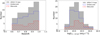 |
Fig. 1. Distributions of redshift (left panel) and intrinsic X-ray luminosity LX (right panel) for the obscured and unobscured AGN samples. The distribution of the combined X-ray sample is over-plotted for reference. |
3.3. X-ray absorption
Out of our 73 sources, 41 have reasonable quality X-ray spectra with over 30 counts while the remaining sourfsee aslces have only hardness ratios available. We first used the column densities given in Lanzuisi et al. (2017, 2018) while for the remaining sources we used the estimates in Marchesi et al. (2016b). In some cases the AGN X-ray spectra may be contaminated by a non-negligible SFR component. This component originates from gas heated by supernova remnants to temperatures of ∼0.8 keV (e.g., Mineo et al. 2012). The luminosity of this component could reach a few times 1041 erg s−1 in the 0.5 − 2 keV band (e.g., Ranalli et al. 2003). Obviously in the case of low-luminosity AGN this component may contribute a significant part of the soft X-ray emission and thus it could affect the column density estimates. We have performed detailed simulations to check the effect of the SFR component using XSPEC (Arnaud 1996). We model the SFR component using the APEC model. We find that for a column density of 1023 cm−2, an AGN X-ray luminosity of L2 − 7 keV ≈ 1043 erg s−1 and a SFR luminosity of L0.5 − 2 keV ∼ 3 × 1041 erg s−1 the column density estimate is not affected. This holds well even in the case of lower column densities of NH = 1022 cm−2. However, in the case of even lower column densities NH < 1021.5 cm−2 in combination with low X-ray AGN luminosities L2 − 7 keV < 1043 erg s−1 and/or high SFR component luminosities in excess of L0.5 − 2 keV ∼ 3 × 1041 erg s−1 the column density estimates could be underestimated.
We divide our sample according to their column density to unobscured or mildly obscured and heavily obscured sources with log NH(cm−2) > 23. The choice of this high threshold column density is dictated by the need to select only bona-fide obscured AGN where the absorption originates in the torus. It has been demonstrated that lower column densities could often be associated with large scale absorption within the galaxy (e.g., Maiolino & Rieke 1995; Malkan et al. 1998; Buchner & Bauer 2017; Circosta et al. 2019; Malizia et al. 2020; D’Amato et al. 2020; Gilli et al. 2022). The obscuration associated with interstellar medium of the host galaxy may be more pronounced at higher redshifts (Scoville et al. 2017; Tacconi et al. 2018). Interestingly, Gilli et al. (2022) predicts that even at a redshift of z ∼ 1 the Galactic column density could be as high as log NH(cm−2) = 22. There are 23 heavily obscured and 50 unobscured or mildly obscured sources. Hereafter, we refer to these as the obscured and unobscured AGN subsamples. Note that in the remaining of the paper when the classification is based on X-ray spectroscopy or hardness ratio we refer to the objects as obscured and unobscured, whereas if the classification is based on optical spectroscopy we refer to the objects as type-2 and type-1 respectively.
4. Analysis
4.1. Spectral Energy distribution fitting using X-CIGALE
In this section we estimate the host galaxy properties, the stellar mass and the star-formation rate. We measure the host galaxy properties of X-ray AGN in our sample, by applying SED fitting using the X-CIGALE code (Boquien et al. 2019). In its latest version (Yang et al. 2020, 2022), CIGALE accounts for extinction of the ultraviolet (UV) and optical emission in the poles of the AGN. At the same time it takes into account the X-ray emission of the AGN in order to better constrain the torus emission. This is performed by means of the αox index which is the spectral slope that connects the 2 keV and the 2500 Å monochromatic emission. For the estimation of the above index, the code requires the intrinsic X-ray fluxes, i.e., X-ray fluxes corrected for X-ray absorption. The improvements that these new features add in the fitting process are described in detail in Yang et al. (2020), Mountrichas et al. (2021b) and Buat et al. (2021).
For the SED fitting process, we use the intrinsic X-ray fluxes estimated in Marchesi et al. (2016b). X-CIGALE uses the αox − L2500 Å relation of Just et al. (2007) to connect the X-ray flux with the AGN emission at 2500 Å. We adopt a maximal value of |Δαox|max = 0.2 that accounts for a ≈2 σ scatter in the above relation.
In the SED fitting analysis, we use the same grid used in Mountrichas et al. (2022c) in the COSMOS field. This allows us to provide a better comparison with the results presented in the above study. Here, we only summarise the modules included in that work. A delayed star formation history (SFH) model with a function form is used to fit the galaxy component. The model includes a star formation burst in the form of an ongoing star formation no longer than 50 Myr (Buat et al. 2019). The Bruzual & Charlot (2003) single stellar population template is used to model the stellar emission. Stellar emission is attenuated following Charlot & Fall (2000). The dust heated by stars is modelled following Dale et al. (2014). The SKIRTOR template Stalevski et al. (2012, 2016) is used for the AGN emission. SKIRTOR assumes a clumpy two-phase torus model, based on 3D radiation-transfer. All free parameters used in the SED fitting process and their input values, are presented in Table 2. In Fig. 2, we present example SED fits for four obscured and four unobscured AGN.
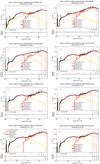 |
Fig. 2. Example SED fits of both obscured (17, 39, 130, 147) and unobscured (77, 106, 137, 209) AGN. |
Models and values for their free parameters used by X-CIGALE for the SED fitting.
4.2. Quality examination
4.2.1. Poor SED fits
We exclude SEDs with poor fits, in order to constrain our analysis only to the sources with reliable host galaxy measurements. For that purpose, we consider only sources for which the reduced χ2,  . This value has been used in previous studies (e.g., Masoura et al. 2018; Buat et al. 2021) and is based on visual inspection of the SEDs. Following this criterion, we have excluded seven sources from further analysis.
4.2.2. SFR
As Zou et al. (2019) pointed out, for sources undetected by Herschel, SFRs derived from SED fitting may be affected by contamination from AGN emission at UV to optical wavelengths. This contamination could be more significant in the case of type-1 AGN. In the Zou et al. (2019) sample, only 32% of the sources had detection in at least one Herschel band. They derived SFR estimates by using single band Herschel photometry and they compared with the SED SFR. They found that although the single band SFRs are overestimated by a factor of a few compared to the SED fits, there is no systematic difference between type-1 and type-2 AGN.
Mountrichas et al. (2022c), used data from the COSMOS fields and showed that the lack of far-IR Herschel photometry (both PACS and SPIRE) does not affect the SFR calculations of X-CIGALE. They used 742 AGN (60% of their total X-ray sample) that have been detected by Herschel. For these sources, they performed SED fitting with and without Herschel bands, using the same parametric space. The results are shown in their Fig. 4. The mean difference of the log(SFR) measurements is 0.01 and the dispersion is σ = 0.25.
In our case, the far-IR photometry available is way more solid. As described in Sect. 3, all of our sources have PACS photometry available, while there are only 23 sources which lack Herschel SPIRE photometry. As an additional check we examine the CIGALE SFR Bayesian errors. We found that the median relative SFR errors (error/measurement) are 0.53 and 0.78 for the unobscured and obscured AGN, respectively. This further supports the fact that our SFR measurements are not contaminated by UV and optical light in the case of unobscured AGN. We note that the median logSFR is 0.41 and 0.18 for the unobscured and unobscured AGN. The corresponding median SFR errors are 0.36 and 0.21 respectively.
4.3. Derivation of the normalised star-formation
A widely applied method to compare the SFR of AGN with that of galaxies, is to use analytical expressions from the literature. Schreiber et al. (2015) describe the SFR-M⋆ correlation, known as the main sequence (Elbaz et al. 2007; Speagle et al. 2014). The estimated parameter is the SFRNORM, defined as the ratio of the SFR of an AGN with M⋆ at redshift z relative to the SFR of normal galaxies at the same stellar mass and redsift. Results from studies that followed this approach (e.g., Mullaney et al. 2015; Masoura et al. 2018, 2021; Bernhard et al. 2019; Torbaniuk et al. 2021) may suffer from systematics. These could be caused by the fact that different methods are applied for the estimation of the host galaxy properties (SFR, M⋆) of AGN and galaxies.
A more advanced approach, is to compare the SFR of AGN with that from a control galaxy, i.e., a non-AGN sample that has been selected by applying the same criteria (e.g., photometric coverage) as the AGN sample and for which the galaxy properties have been calculated following the same method (e.g., SED fitting). This method has been applied by Shimizu et al. (2015, 2017) in hard (14–195 keV) X-ray selected AGN from the Swift/BAT and more recently by Mountrichas et al. (2021c, 2022a,2022c). The limitation of this method is the available number of reference galaxies at a given M⋆, z bin (Pouliasis et al. 2022). Here, we compare the SFR of X-ray AGN with that of normal galaxies. We apply the same SED fitting analysis in both datasets and we require the availability of the same photometric bands. The reference sample is drawn from the HELP catalogue (Shirley et al. 2019). There are about ∼2.5 million galaxies in the COSMOS field of which ∼500 000 are in the 1.38 deg2 of UltraVISTA (see also Laigle et al. 2016). There are ∼230 000 galaxies, after we exclude X-ray sources, that meet the photometric requirements we have set on the X-ray sample.
We compare the SFR of X-ray AGN with that of galaxies, using the SFRnorm parameter. We derive the SFRnorm following the method described in Mountrichas et al. (2022c). In more detail, the SFR of each X-ray source is divided by the SFR of galaxies from the reference catalogue. These galaxies are selected to have stellar mass that differs ±0.1 dex from the stellar mass of the AGN and is found within ±0.075 × (1 + z) from the X-ray source. The median value of these ratios is used as the SFRnorm of each AGN. In these calculations, each source is weighted based on the uncertainty on the SFR and M*. The most reliable estimates refer to X-ray sources for which the SFRnorm has been derived using at least 20 galaxies from the reference catalogue. However, this necessarily lowers to less than ten galaxies when we consider only the most massive systems (11.5 < log [M*(M⊙)] < 12.0).
4.4. Black hole masses and Eddington ratios
One of the main measurements coming from the high resolution LEGA-C spectra is the velocity dispersion (van der Wel et al. 2016). These have an error of only 0.08 dex. Eight sources (6 unobscured and two obscured AGN) do not have a measurement of the velocity dispersion available and hence are excluded from the Eddington ratio analysis. The velocity dispersions can provide a good proxy of the black hole mass MBH. Ferrarese & Merritt (2000), Gebhardt et al. (2000) found a strong correlation between the black hole mass and the stellar velocity dispersion. Merritt & Ferrarese (2001) proposed the following relation between the above quantities.
where σ200 is the stellar velocity dispersion in units of 200 km s−1.
The Eddington luminosity is the maximum luminosity that can be emitted by the AGN. This is defined by the balance between the radiation pressure and the gravitational force exerted by the black hole.

The Eddington ratio is defined as the ratio of the bolometric luminosity and the Eddington luminosity, λEDD = LBOL/LEDD. The bolometric luminosity is usually determined from the X-ray luminosity (Marconi et al. 2004; Vasudevan et al. 2013; Lusso et al. 2012). We use here the most recent relation calibrated in Duras et al. (2020). These bolometric corrections take into account both the X-ray luminosity and they differentiate between obscured and unobscured AGN.
5. Results and discussion
In this section we present the distributions of the age of the host galaxy, the SFR, the stellar mass the Eddington ratio and velocity dispersion separately for the obscured and unobscured AGN populations.
5.1. Normalisation of the obscured and unobscured samples
Since the z and LX distributions are different for obscured and unobscured AGN (Fig. 1), we need to compare the host galaxy stellar mass and age distributions by normalising on luminosity and redshift. This is done with the use of control samples. We follow the method of Zou et al. (2019) for the creation of the control samples, dividing the log LX − z plane into a grid with Δz = 0.1 and Δlog LX = 0.5 dex (see Fig. 3). We randomly select N1(zi, Lj) unobscured sources as well as the same number of obscured sources N2(zi, Lj) in the considered i,j grid element. After repeating the procedure in each redshift, luminosity bin, we end up with new unobscured and obscured samples with similar distributions of z and LX. The obscured and unobscured control samples contain 73 sources each i.e. the total number of sources in our sample.
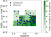 |
Fig. 3. Distribution in the redshift and intrinsic luminosity plane for the obscured and unobscured AGN. The grid is used to assign weights in different z, Lx bins in order to take into account the different luminosity and redshift distributions of obscured and unobscured AGN (see Sect. 5.1). |
5.2. Age indicators
We have used the amplitude of the 4000-Å break and the Hδ absorption line (Worthey & Ottaviani 1997) as the age indicators of the host galaxies. The Dn(4000) index quantifies the strength of the calcium break at 4000 Å (Balogh et al. 1999). This is defined as Dn = F4050/F3900. This break is prominent in older and metal-rich stellar populations. It is caused by the CAII absorption doublet and by line blanketing of metal lines in stellar atmospheres. Metals in the outer layer of a star’s atmosphere absorb some of the star’s radiation and re-emit it at redder wavelengths. Then galaxies which experienced a recent episode of star-formation have a smaller Dn index because of the presence of young stars. Another commonly used age indicator is provided by the Balmer lines which are most prominent in the youngest stars. Absorption takes place mostly in A stars which have large amounts of neutral material available. This has been interpreted by Dressler & Gunn (1983) as an indication that that the SFR burst ended 0.5–1.5 Gyr before the observation. At the redshifts probed here higher order Balmer lines such as Hδ, are observed as the redder lines shift out of frame. The strength of absorption features is often quantified using the Lick indices. The Lick indices measure the flux in the absorption line comparing it with the flux in a nearby pseudo-continuum. This defines the strength of the line: I = (λ2 − λ1)(1 − FL/FC) where where λ2 − λ1 is the width of the passband used to measure the index and FC and FL are the fluxes of the continuum and the line respectively (for details see Worthey & Ottaviani 1997). The units of Hδ are given in Å. For more details on the extraction of the Dn and Hδ indices are given in Straatman et al. (2018) and van der Wel et al. (2021). We note that the presence of a strong AGN may affect the Dn and Hδ values. For example, regarding the Calcium break, this could happen if the relative contribution of the AGN to the galaxy R = FAGN/FGal is different in the passbands centred at 3900 Å and 4050 Å. The ratio R above can be determined from our SED fitting. We found that the ratios are very close to unity and then the resulting corrections are very small.
In Fig. 4 we present the plot with the age indicators of our sample compared to the LEGA-C galaxy sample. We colour-code our sources using (a) the column density (b) the stellar mass (c) the specific star-formation rate (d) the normalised star formation rate and (e) Eddington ratio (f) velocity dispersion. Note that this plot has not being weighted for the different luminosity and redshift distributions of the obscured and unobscured objects.
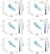 |
Fig. 4. Age indicators Hδ − Dn(4000) plots for our sample. The triangles and the squares denote the obscured and the unobscured AGN respectively. The colour-coded key gives the value of the (a) intrinsic AGN column density. The dotted lines gives the contours that include 68% and 99% of the LEGA-C galaxy population (b) stellar mass, (c) specific SFR, (d) normalised SFR, (e) Eddington ratio, and (f) stellar velocity dispersion. The obscured and unobscured AGN samples have not been corrected for differences in their luminosity and redshift distribution. |
The locus of galaxies is forming a sequence moving from high (low) values of Dn ∼ 2 (Hδ ∼ −3) to low (high) values of Dn ∼ 1.2 (Hδ ∼ 5). Large deviations from this locus are often used as an indicator of recent bursts of star formation (Kauffmann et al. 2003). It can be seen that the galaxies are separated in two groups. The old group clusters around (Dn, Hδ)≈(1.8, 0) while the young group populates the area around (Dn, Hδ)≈(1.3, 5.5). The AGN occupy both the old and young cloud but with some tendency towards the young cloud. In particular, the unobscured AGN populate more frequently the young cloud compared to the obscured AGN. The obscured AGN appear to have cc intermediate ages populating the region (Dn, Hδ)≈(1.5, 2.5). The above differences can be more clearly seen in the histogram of Dn (Fig. 5). We note that in this figure the samples have been normalised in order to follow the same luminosity and redshift distributions (see Sect. 5.1). It is apparent that the unobscured population is associated mainly with young galaxies. Instead the obscured population occupies an area in the middle of the young and old cloud. More specifically, the obscured and unobscured AGN population have a median Dn value of 1.53 and 1.40 respectively. The K-S test shows that the two populations have different distributions in the Dn at a statistically significant level (see Table 3). Following standard practice, we adopt 2σ (p-value = 0.05) as the threshold for a ‘statistically significant’ difference in host-galaxy properties. The distribution of Hδ (Fig. 5) shows that both populations present a peak around Hδ ∼ 3 albeit the host galaxies of the unobscured AGN present also a large tail at younger ages Hδ ≈ 5.
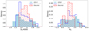 |
Fig. 5. Distribution of the Dn (left panel) and Hδ (right panel) age indicators for the obscured and unobscured AGN samples. The samples have been normalised in order to follow the same luminosity and redshift distribution (see Sect. 5.1 for details). We over-plot the distribution of the LEGA-C galaxies for reference. |
Median values and K-S statistics for the obscured and unobscured sample.
Silverman et al. (2009) have investigated the ages of the host galaxies of XMM-Newton selected AGN in the XMM-Newton COSMOS field using the calcium break Dn(4000). They find an increased AGN fraction among the galaxies with younger populations with 1 < Dn(4000) < 1.4. These young galaxies are actively star-forming as indicated by their blue rest frame U-V colour as well as the strength of the [OII] line. Finally, Hernán-Caballero et al. (2014) analyse the stellar populations in the host galaxies of 53 X-ray selected optically dull active galactic nuclei (AGN) at a redshift range of 0.34 < z < 1.07 from the Survey for High-z Absorption Red and Dead Sources (SHARDS). They find a highly significant excess of AGN hosts with Dn(4000)≈1.4, as well as a deficit of AGN in intrinsically red galaxies. Therefore our results are in good agreement overall with those of Hernán-Caballero et al. (2014) as far as the total AGN population is concerned. An additional important result of our analysis is that we separate for the first time the X-ray selected AGN in obscured and unobscured objects finding a significant difference in their host galaxy ages.
5.3. Stellar ages
From the Dn and Hδ values derived above it becomes evident that the obscured AGN population is associated on average with older host galaxies, compared to the unobscured AGN population. It is instructive to derive the approximate stellar ages of these populations. The CIGALE code provides stellar ages estimates. However, Mountrichas et al. (2022b) caution that the CIGALE estimates have limited accuracy if they are not combined with Dn and Hδ measurements. Hence, they developed a variant of the CIGALE code which uses both these indices to estimate the mass weighted galaxy ages. As this code is not publicly available, we can rely on their galaxy age methodology. This is possible because the LEGA-C COSMOS sample used by Mountrichas et al. (2022b) is practically identical to our sample and moreover they use the same parameter grid for their SED fitting.
Mountrichas et al. (2022b) derive the spectral age index using both the Dn and EW(Hδ) measurements. This index combines Dn and Hδ to construct the distribution of galaxies along the diagonal distribution on the Dn − Hδ plane (see Wu et al. 2018). They derive a spectral age index (S.A.I.) defined as −2.40 × Dn − EW(Hδ)+4.36 (priv. comm.). They combine the S.A.I. with the CIGALE mass weighted age estimates to create the S.A.I – age plot. Using this plot, the combination of EW(Hδ) and Dn translates to a mass-weighted galaxy age. We use the median Hδ and EW(Hδ) estimates to obtain the exact S.A.I. for our obscured and unobscured samples. We obtain values of 3280 and 2740 Myr for the mass-weighted ages of the host galaxies of the obscured and unobscured populations respectively.
5.4. Distribution of stellar mass
Here, we examine whether there is any difference in the stellar mass distributions of the obscured and the unobscured AGN population. In Fig. 4 (top right panel) we show the distribution of the stellar mass as a function of the two age indicators Dn and Hδ. There is a preponderance of AGN associated with low mass galaxies with ∼ log M⋆(M⊙) < 11.2 in the young cloud (Dn < 1.5). Most of these low mass galaxies are associated with unobscured AGN. The difference between the galaxy masses of the two populations can be better quantified in the histograms of the stellar mass shown in Fig. 6. In this figure and subsequent histogram figures the y-axis (density) refers to the frequency histogram so that the sum of all bins is equal to one. The two distributions are different with the obscured AGN population being skewed towards higher stellar mass (p-value = 1 × 10⁻³). Zou et al. (2019) first noticed that the stellar masses of type-2 AGN are on average higher that that of type-1 AGN (but see Suh et al. 2019). Mountrichas et al. (2021a) confirmed this result in the XMM-XXL field. However, the division between type-1 and type-2 in both Zou et al. (2019) and Mountrichas et al. (2021a) is based on optical spectroscopy. Here, we find probably for the first time a difference in stellar mass between obscured and unobscured AGN samples based on X-ray spectroscopy and hardness ratios. Previous works failed to identify a difference in stellar mass between the two populations (Merloni et al. 2014; Masoura et al. 2021; Mountrichas et al. 2021c). However, in the above works the column density cut-off between obscured and unobscured AGN was set at much lower column densities log NH(cm−2) = 22 or log NH(cm−2) = 21.5. We re-examine this apparent controversy in Sect. 5.10. The difference in stellar mass could possibly signify a difference in the age of the two populations. This is in the sense that older galaxies had more time to increase their mass through galaxy mergers.
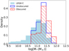 |
Fig. 6. Distribution of M* for the obscured and unobscured AGN samples. The distribution refers to the frequency histogram so that the sum of all bins equals unity. The distribution has been weighted taking into account the redshift and luminosity distributions of obscured and unobscured AGN. We over-plot the distribution of the LEGA-C galaxies for reference. |
5.5. Star-formation rate
The distribution of the specific SFR, sSFR, defined as the SFR per stellar mass as a function of the age indicators is presented in Fig. 4 (middle right panel). We notice a trend where the majority of the AGN with high sSFR are hosted by galaxies with the youngest ages. Moreover, these appear to be primarily associated with unobscured AGN. This can be more clearly seen in Fig. 7 we plot the histogram of the sSFR for the obscured vs. the unobscured AGN. The two distributions are different at a statistically significant level yielding p-value ≈ 1 × 10⁻⁴.
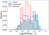 |
Fig. 7. Distribution of the specific SFR, sSFR, for the obscured and unobscured AGN samples. The samples have been weighted in order to follow the same X-ray luminosity and redshift distribution (see Sect. 5.1 for details). The sSFR distribution of the LEGA-C galaxies is overplotted for reference. |
The SFRNORM results can provide a more accurate picture of the AGN SFR relative to galaxies of the same stellar mass and redshift. Our SFRNORM results are presented in Fig. 4 (middle right panel) as a function of the age of the host galaxy. There is a tendency for the highly star-forming systems to be associated with young galaxies regardless of the AGN type. Most AGN host galaxies with logSFRNORM > 0.5 have a calcium break value of Dn < 1.5. In Fig. 8 we compare the SFRNORM histograms for obscured and unobscured AGN. Both the obscured and unobscured AGN populations cluster around the main sequence of star-formation (logSFR = 0). The median logSFRNORM equals −0.09 and 0.03 for the obscured and unobscured AGN respectively. The obscured AGN have an SFRNORM skewed towards lower values compared to the unobscured AGN.
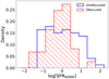 |
Fig. 8. Distribution of SFRNORM for the obscured and unobscured AGN samples. The samples have been weighted in order to follow the same X-ray luminosity and redshift distribution (see Sect. 5.1 for details). |
There has been no concrete evidence in the literature that the SFR properties of X-ray selected obscured and unobscured AGN are different regardless of whether the separation between the two populations is performed using optical spectroscopy (Zou et al. 2019; Mountrichas et al. 2021a) or X-ray spectroscopy (Masoura et al. 2021). Mountrichas et al. (2021a) studied the X-ray selected AGN in the XMM-XXL field, in the redshift range z = 0 − 1, classifying them as type-1 or type-2 on the basis of optical spectroscopy. They estimate logSFRNORM ∼ 0 for both types of AGN. Masoura et al. (2021) studied the X-ray selected AGN in the same field performing the classification between unobscured and obscured AGN based on Bayesian X-ray hardness ratios and applying a column density dividing threshold of log NH(cm−2) = 21.5. Finally, Mountrichas et al. (2021c) studied the SFRNORM for obscured and unobscured AGN in the XBOOTES field applying a hardness ratio classification using column density dividing threshold of log NH(cm−2) = 22. Both works find that the SFRNORM distributions are similar for the two populations.
5.6. Eddington ratio distribution
The Eddington ratio λE distribution provides another key element in the study of the AGN demographics. It has been suggested that the radiation pressure exerted on the obscuring screen regulates the AGN obscuration (Fabian et al. 2008, 2009; Ricci et al. 2017) in the sense that the high radiation pressure pushes the obscuring torus further away and therefore decreases the obscuration. According to this model high Eddington ratios should correspond primarily to unobscured AGN while the obscured AGN should have lower Eddington ratios. Ricci et al. (2017) present the NH − λEDD plane for hard X-ray selected AGN where they demonstrate that there is a strong separation between the obscured and unobscured AGN with the former occupying primarily the low λ high NH region. More recently, Ananna et al. (2022) has provided a comprehensive study of the Eddington ratio distribution for obscured and unobscured AGN in the local Universe using the Swift/BAT AGN sample. They find that the Eddington ratio distribution of obscured AGN is significantly skewed towards lower Eddington ratios.
In Fig. 9, we present the column density versus the Eddington ratio diagram. Our obscured sources have relatively low log[λEDD]< − 0.8. All lie above the effective Eddington limit where the outward radiation pressure on gas is equal to the inward gravitational pull. We present the distribution of the Eddington ratio as a key in the colour-coded diagram of Fig. 4. The histogram of the λE is shown in Fig. 10. There is a tendency for obscured AGN to populate the lower Eddington ratio bins with a peak at λE ≈ −2. The two distributions are different at a highly statistically significant level according to the K-S test (p-value ∼ 3 × 10⁻⁶). Therefore our results are in reasonable agreement with the findings of Ananna et al. (2022) in the local Universe.
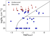 |
Fig. 9. Column density versus the Eddington ratio. The solid curve represents the effective Eddington ratio where the outward radiation pressure on gas is equal to the inward gravitational pull. The horizontal line denotes the column density value where the obscuration could come from large scale clouds in the galaxy. |
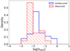 |
Fig. 10. Distribution of log[λEDD] for the obscured and unobscured AGN samples. |
5.7. The relation between the galaxy age and stellar mass
In the previous sections we argued that the host galaxies of the obscured AGN are on average older than those of the unobscured AGN. The mass distribution of obscured AGN appears to be skewed towards higher masses. At the same time, the host galaxies of obscured AGN appear to have lower star-formation rates. All the above could suggest that the mass of the host galaxy is directly related to its age. We plot the galaxy age Dn vs. stellar mass in Fig. 11 (upper panels) using as colour keys the sSFR and the Eddington ratio. There does not appear to be an obvious relation between the stellar mass and the age in the sense that the host galaxies with a typical stellar masses of M⋆ = 1011 − 11.5 M⊙ cover a very wide range of galaxy ages. The relation between the black hole mass and host galaxy age appears to apply as well to the normal (non-AGN) galaxies which have a mass of M⋆ > 1010.5 M⊙. In contrast, lower mass galaxies are associated with young galaxies (Dn ≈ 1.2).
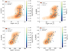 |
Fig. 11. Relation between galaxy age and stellar mass and black hole mass. Top panel: calcium break Dn as a function of the stellar mass. Lower panel: calcium break as function of the velocity dispersion σ⋆. In the right and left hand plots the colour key represents the sSFR and the Eddington ratio, respectively. The contours represent the LEGA-C galaxy population. |
5.8. The relation between the galaxy age and black hole mass
In Fig. 11 (lower panel), there appears to be a trend for a correlation between the host galaxy age and σ⋆ in the sense that the older the age the largest the velocity dispersion σ⋆ that is the more massive the black hole. This trend is weakened by couple of obscured AGN which have young ages Dn < 1.4 relative to their velocity dispersion σ⋆ > 250 km s−1. Note that the relation between galaxy age and stellar velocity dispersion is more prominent in the underlying galaxy population. Regarding the AGN population, the youngest AGN host galaxies, are those which show the highest Eddington ratios and highest star-formation rates.
5.9. Normalising with stellar mass
In the previous sections we have demonstrated that the ages of the host galaxies of obscured AGN are higher compared to the non-obscured ones. The normalisation or weighing between the two populations was based on control samples using the X-ray luminosity and redshift (Zou et al. 2019; Mountrichas et al. 2022a). As the masses of the obscured AGN are higher than those of the unobscured ones, we explore whether the stellar mass could be the underlying reason for the difference in age. We perform the weighting method using control samples that has been described in Sect. 5.1. The results are presented in Table 4. The differences in the age indicators Dn and Hδ again imply that the age of the host galaxies of the obscured AGN population is older at a statistically significant level. The Dn and Hδ indices distributions are presented in Fig. 12.
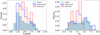 |
Fig. 12. Distributions of the Dn (left panel) and Hδ (right panel) age indicators for the obscured and unobscured AGN samples. The samples have been weighted in order to follow the same redshift and stellar mass distribution (see Sects. 5.1 and 5.9 for details). We over-plot the distribution of the LEGA-C galaxies for reference. |
Median values and K-S statistics for the obscured and unobscured sample in the case of normalising the samples with M⋆.
5.10. The effect of the absorbing column density cut
In Sect. 3 we argued that we need to adopt a high absorbing column density cut to make sure that our the obscuration of our sources originates in the torus rather than the host galaxy. Here, we investigate the effect that a lower column density cut would have on our results. We explore the usually adopted value of log NH(cm−2) = 22 which is most commonly used as the dividing line between obscured and unobscured AGN. In addition, we investigate the effect of an even lower cut-off of log NH(cm−2) = 21.5. This column density dividing line has been proposed by Merloni et al. (2014) who argue that this brings the samples of type-1 and type-2 objects (selected on the basis of optical spectroscopy) in relatively good agreement with the unobscured and unobscured AGN samples (selected on the basis of X-ray spectroscopy). We construct anew the obscured and unobscured AGN samples based on the above criteria and examine their host galaxy properties. In Fig. 13 we present the distributions of the calcium break, the stellar mass, the sSFR, Eddington ratio for all three cuts. We present the new p-values for the Kolmogorov-Smirnov tests in Table 5. From the above plot and the table it becomes evident that the differences between the obscured and the unobscured AGN are less pronounced. In particular, it appears that there is no difference in Dn for obscured and unobscured AGN. The stellar mass appears to be different at log NH(cm−2) = 22 while at the dividing threshold of log NH(cm−2) = 21.5 the stellar mass distributions are similar. The effect of column density cut can be visualised in Fig. 14 where we plot the p-values for the different parameters as a function of the column density.
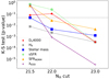 |
Fig. 13. Kolmogorov-Smirnov p-values for the comparison of the obscured and unobscured population parameters as a function of the column density cut: (a) stellar mass (blue, square box), (b) Dn(4000) (red, star), (c) sSFR (green, circle), (d) SFRNORM (orange, triangle), and (e) Eddington ratio (purple, cross). The horizontal line denotes the 95% confidence level. |
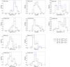 |
Fig. 14. Distributions of : (a) Stellar mass, (b) calcium break Dn(4000), (c) sSFR, (d) SFRNORM, and (e) Eddington ratio for the obscured (upper panel) and unobscured AGN (lower panel). The distributions are shown for three column density NH cuts: log NH(cm−2) = 23 (sold black line), log NH(cm−2) = 22 (blue dash line) and log NH(cm−2) = 21.5 (yellow dot line). |
Median values and K-S statistics for lower column density NH cuts.
5.11. Comparison with theoretical models
Many theoretical models assert that AGN can be triggered by major mergers of massive gas rich galaxies (e.g., Hopkins et al. 2006, 2010). The mergers cause the gas to lose angular momentum and eventually to fall in the centre of the galaxy. These mergers could resemble the IR luminous galaxies in the local Universe (Sanders et al. 1988). The nucleus should remain heavily obscured in this initial stage of the AGN. Observational evidence suggests that a large fraction of heavily obscured AGN are associated with mergers (Koss et al. 2010, 2018; Kocevski et al. 2015; Lanzuisi et al. 2018). The nuclear gas will either feed the central SMBH or will be consumed in star-formation. This phase is marked by co-existence of copious star-formation and AGN activity. When the AGN increases its Eddington ratio, powerful outflows push away the surrounding material in a short outburst phase (see e.g., Fabian 2012; King & Pounds 2015). In the Colour Magnitude Diagram, u − r vs. Mr, the galaxy should move from the red cloud (absorbed phase) to the blue cloud (intense star formation phase) to the green valley and eventually back to the red cloud when both the star formation and the AGN turn off (Hickox et al. 2009).
There is observational evidence that the major mergers may not be the dominant AGN triggering mechanism (see Kormendy & Ho 2013). Schawinski et al. (2011) and Kocevski et al. (2012) find that most moderate luminosity AGN are hosted by disk galaxies in the redshift range z = 1.5–3. Also Georgakakis et al. (2009) find that AGN hosted by disk galaxies contribute an appreciable fraction of the AGN luminosity density at z ≈ 0.8. Then it is likely that secular processes drive gas to the centre of the galaxy and trigger the AGN (Draper & Ballantyne 2012). These secular processes include supernova winds, minor mergers, interactions with other galaxies or cold accretion flow (Kormendy & Kennicutt 2004).
The current work shows that the host galaxies of the obscured AGN are on average older than those of obscured AGN. This is rather at odds with the major merger scenario where the obscured phase marks the first stage of the AGN. As the host galaxies of the (moderate luminosity) obscured AGN in the COSMOS field appear to be at a later evolution stage compared to the unobscured AGN, this may be more suggestive of secular evolution. This obscured phase comes as a second phase following the high SFR and high Eddington ratio phase. In the obscured phase, both the star-formation and the AGN accretion are abated. The low Eddington ratios do not appear to be sufficiently high to clear the surrounding gas. Alternatively when the Eddington ratios decrease the surrounding gas can fall back towards the centre increasing the obscuration.
5.12. Outstanding questions
The current work provides some interesting insights on the host galaxy age of the obscured and unobscured AGN population. It also suggests the presence of significant differences between the host galaxy masses as well as their SFR. These differences may be explained by the difference in galaxy age. However, there are remaining questions that need to be addressed in order to fully understand the differences of galaxy properties in the obscured and unobscured AGN populations. These questions are mostly related to the classification between the obscured (type-2) and unobscured (type-1) AGN, and can be summarised as follows
(a) Column density limit. The differences in the host galaxy age appear to be pronounced only for the heavily obscured sources with log NH(cm−2) = 23. There are no differences between the age of the obscured and unobscured populations when the column density threshold becomes log NH(cm−2) = 22 or log NH(cm−2) = 21.5. The difference in stellar mass probably persists even at lower column densities of log NH(cm−2) = 22. This is in agreement with previous results by Mountrichas et al. (2021c) in the XBOOTES field. Interestingly, Lanzuisi et al. (2017) and Buchner & Bauer (2017) show that there is a strong correlation between the absorbing column density and the stellar mass in X-ray selected AGN suggesting a difference in stellar mass between the obscured and unobscured AGN.
(b) Optical versus X-ray classification. Similar controversies occur when the classification between obscured and unobscured AGN is based on X-ray spectroscopy (or hardness ratio) and optical spectroscopy (i.e. redenning). Although we found a significant difference between the ages of obscured and unobscured AGN at a redshift of z ∼ 0.7, the work on optically selected SDSS AGN by Kauffmann et al. (2003) finds comparable ages for type-1 and type-2 AGN at lower redshifts z < 0.3.
(c) Luminosity. There is a possibility that the differences with previous results may not be attributed to the classification method but rather on the luminosity. Owing to the deeper flux limit, the AGN in the COSMOS field are less luminous compared to those in XBOOTES and XMM-XXL which have been used to compare the host galaxy properties of obscured and unobscured sources (e.g., Masoura et al. 2021; Mountrichas et al. 2021c). On the other hand, studies that have classified their AGN based on optical criteria have either used the lower LX sources of the COSMOS field (e.g., Zou et al. 2019) or have restricted their analysis to low luminosity systems at low redshift (Mountrichas et al. 2021a). It is then likely that the differences found in the host galaxy properties of type-1 and type-2 AGN are because of their lower luminosities of the AGN utilised rather than the different classification method (X-ray vs. optical).
6. Summary
We examine the ages of the host galaxies of Chandra X-ray selected AGN in the COSMOS field in combination with other properties such as the stellar mass, the SFR and finally the SMBH Eddington ratio. The ages are explored using the calcium break and the Balmer Hδ absorption line obtained from the LEGA-C VLT/VIMOS survey. Accurate stellar masses and SFR are derived using the spectral energy distribution code CIGALE. We compare for the first time the ages of the host galaxies of obscured and unobscured X-ray selected AGN. Our sample consists of 50 unobscured or mildly obscured (log NH(cm−2) < 23) and 23 heavily obscured AGN (log NH(cm−2) > 23) in the redshift range 0.6 < z < 1. One of our goals is to test the predictions of evolutionary unification models which assert that heavily obscured sources mark the birth phase of the AGN. Our main results can be summarised as follows.
The AGN occupy the full range of ages from old systems to young galaxies. They preferentially lie around a value of the calcium break of Dn ≈ 1.4 − 1.5. This implies that AGN are associated with galaxies that have intermediate ages. Our findings corroborate previous results by Hernán-Caballero et al. (2014) but they are rather in tension with other results in the COSMOS field which assert that the X-ray selected AGN are preferentially associated with young star-forming systems (Silverman et al. 2009).
One of the main results of this work is that obscured AGN are associated with older galaxies having a median value for the calcium break of Dn ≈ 1.53 compared to unobscured AGN which have Dn ≈ 1.40. A Kolmogorov-Smirnov test finds that the Dn distributions of obscured and unobscured AGN are different at a highly significant level (p-value 3 × 10⁻⁴).
There is some evidence that the stellar masses of obscured AGN are skewed towards higher values compared to those of unobscured AGN p-value = 1.3 × 10⁻³. This result is in line with earlier findings based on the classification between type-1 and type-2 AGN following optical spectroscopy (Zou et al. 2019; Mountrichas et al. 2021a; Koutoulidis et al. 2022). However, it is the first time that this is reported based on classification resulting from X-ray spectroscopy. The difference in stellar mass is consistent with the older ages of obscured AGN found above under the assumption that older galaxies are assocciated with more massive galaxies (Kauffmann et al. 2003; Wu et al. 2018; Wilman et al. 2008). Our results on the different ages of the host galaxies of the obscured and unobscured AGN populations still apply when we normalise our samples according to stellar mass.
The SFR of obscured AGN appears to be lower than that of unobscured AGN as demonstrated both by the comparison of the sSFR and the more sensitive SFRNORM distributions for the obscured and the unobscured AGN. This combined with the finding above that the Eddington ratios in unobscured AGN are significantly higher than those of obscured AGN implies that high levels of SFR go hand in hand with high accretion rates possibly fed by the same gas depot.
We have demonstrated that the above results regarding the host galaxy ages probably do not persevere for lower column densities (log NH(cm−2) = 21.5 or 22).
Finally, the Eddington ratio distribution of the obscured AGN are skewed towards lower values compared to the unobscured AGN. This supports a scenario where the shape torus is regulated by the AGN radiation pressure as suggested by Ananna et al. (2022).
All the above have implications for the evolutionary unification models which are based on massive galaxy mergers. These models postulate that an AGN begins its life in a highly obscured phase. When the Eddington rate increases the obscured screen is pushed away by the radiation pressure and the AGN passes in an unobscured phase which is accompanied by intense star-formation. The results presented in this paper support that the obscured AGN on average are not hosted by the youngest galaxies in contrast to the above scenarios. As the Eddington ratios of obscured AGN are lower than those of unobscured AGN, this supports a scenario where the obscured AGN did not reach sufficiently high levels of radiation pressure to blow away the obscuring screen. Instead, the lower SFR in obscured AGN in combination with their lower Eddington ratios may be related to limited availability of fuel in the vicinity of the black hole. As there are rather diverging results on the gas content of AGN (Maiolino et al. 1997; Perna et al. 2018), this hypothesis needs to be systematically explored using future ALMA observations of AGN.
Acknowledgments
The authors are grateful to the anonymous referee for his careful reading of the manuscript and numerous constructive comments. IG acknowledges financial support by the European Union’s Horizon 2020 programme “XMM2ATHENA” under grant agreement No 101004168. The research leading to these results has received funding (EP and IG) from the European Union’s Horizon 2020 Programme under the AHEAD2020 project (grant agreement n. 871158). GM acknowledges support by the Agencia Estatal de Investigación, Unidad de Excelencia María de Maeztu, ref. MDM-2017-0765. We acknowledge the use of LEGA-C data which have been obtained with the ESO Telescopes at the La Silla Paranal Observatory.
References
- Aird, J., Coil, A. L., Moustakas, J., et al. 2012, ApJ, 746, 90 [CrossRef] [Google Scholar]
- Aird, J., Coil, A. L., & Georgakakis, A. 2019, MNRAS, 484, 4360 [NASA ADS] [CrossRef] [Google Scholar]
- Ananna, T. T., Weigel, A. K., Trakhtenbrot, B., et al. 2022, ApJS, 261, 9 [NASA ADS] [CrossRef] [Google Scholar]
- Antonucci, R. 1993, ARA&A, 31, 473 [Google Scholar]
- Arnaud, K. A. 1996, ASP Conf. Ser., 101, 17 [Google Scholar]
- Balogh, M. L., Morris, S. L., Yee, H. K. C., Carlberg, R. G., & Ellingson, E. 1999, ApJ, 527, 54 [Google Scholar]
- Banerji, M., Jones, G. C., Carniani, S., DeGraf, C., & Wagg, J. 2021, MNRAS, 503, 5583 [Google Scholar]
- Bernhard, E., Grimmett, L. P., Mullaney, J. R., et al. 2019, MNRAS, 483, L52 [NASA ADS] [CrossRef] [Google Scholar]
- Blecha, L., Snyder, G. F., Satyapal, S., & Ellison, S. L. 2018, MNRAS, 478, 3056 [Google Scholar]
- Boquien, M., Burgarella, D., Roehlly, Y., et al. 2019, A&A, 622, A103 [NASA ADS] [CrossRef] [EDP Sciences] [Google Scholar]
- Brown, A., Nayyeri, H., Cooray, A., et al. 2019, ApJ, 871, 87 [NASA ADS] [CrossRef] [Google Scholar]
- Bruzual, G., & Charlot, S. 2003, MNRAS, 344, 1000 [NASA ADS] [CrossRef] [Google Scholar]
- Buat, V., Ciesla, L., Boquien, M., Małek, K., & Burgarella, D. 2019, A&A, 632, A79 [NASA ADS] [CrossRef] [EDP Sciences] [Google Scholar]
- Buat, V., Mountrichas, G., Yang, G., et al. 2021, A&A, 654, A93 [NASA ADS] [CrossRef] [EDP Sciences] [Google Scholar]
- Buchner, J., & Bauer, F. E. 2017, MNRAS, 465, 4348 [Google Scholar]
- Chabrier, G. 2003, ApJ, 586, L133 [NASA ADS] [CrossRef] [Google Scholar]
- Charlot, S., & Fall, S. M. 2000, ApJ, 539, 718 [Google Scholar]
- Chen, C.-T. J., Hickox, R. C., Alberts, S., et al. 2013, ApJ, 773, 3 [NASA ADS] [CrossRef] [Google Scholar]
- Chen, C.-T. J., Hickox, R. C., Alberts, S., et al. 2015, ApJ, 802, 50 [Google Scholar]
- Ciotti, L., & Ostriker, J. P. 1997, ApJ, 487, L105 [NASA ADS] [CrossRef] [Google Scholar]
- Circosta, C., Vignali, C., Gilli, R., et al. 2019, A&A, 623, A172 [NASA ADS] [CrossRef] [EDP Sciences] [Google Scholar]
- Civano, F., Marchesi, S., Comastri, A., et al. 2016, ApJ, 819, 62 [Google Scholar]
- Dale, D. A., Helou, G., Magdis, G. E., et al. 2014, ApJ, 784, 83 [Google Scholar]
- D’Amato, Q., Gilli, R., Vignali, C., et al. 2020, A&A, 636, A37 [NASA ADS] [CrossRef] [EDP Sciences] [Google Scholar]
- Di Matteo, T., Springel, V., & Hernquist, L. 2005, Nature, 433, 604 [NASA ADS] [CrossRef] [Google Scholar]
- Draper, A. R., & Ballantyne, D. R. 2012, ApJ, 751, 72 [NASA ADS] [CrossRef] [Google Scholar]
- Dressler, A., & Gunn, J. E. 1983, ApJ, 270, 7 [NASA ADS] [CrossRef] [Google Scholar]
- Duras, F., Bongiorno, A., Ricci, F., et al. 2020, A&A, 636, A73 [NASA ADS] [CrossRef] [EDP Sciences] [Google Scholar]
- Elbaz, D., Daddi, E., Le Borgne, D., et al. 2007, A&A, 468, 33 [NASA ADS] [CrossRef] [EDP Sciences] [Google Scholar]
- Fabian, A. C. 2012, ARA&A, 50, 455 [Google Scholar]
- Fabian, A. C., Vasudevan, R. V., & Gandhi, P. 2008, MNRAS, 385, L43 [NASA ADS] [CrossRef] [Google Scholar]
- Fabian, A. C., Vasudevan, R. V., Mushotzky, R. F., Winter, L. M., & Reynolds, C. S. 2009, MNRAS, 394, L89 [NASA ADS] [CrossRef] [Google Scholar]
- Ferrarese, L., & Merritt, D. 2000, ApJ, 539, L9 [Google Scholar]
- Florez, J., Jogee, S., Sherman, S., et al. 2020, MNRAS, 497, 3273 [NASA ADS] [CrossRef] [Google Scholar]
- Fornasini, F. M., Civano, F., & Suh, H. 2020, MNRAS, 495, 771 [NASA ADS] [CrossRef] [Google Scholar]
- Gebhardt, K., Kormendy, J., Ho, L. C., et al. 2000, ApJ, 543, L5 [CrossRef] [Google Scholar]
- Georgakakis, A., Coil, A. L., Laird, E. S., et al. 2009, MNRAS, 397, 623 [CrossRef] [Google Scholar]
- Gilli, R., Norman, C., Calura, F., et al. 2022, A&A, 666, A17 [NASA ADS] [CrossRef] [EDP Sciences] [Google Scholar]
- Glikman, E., Lacy, M., LaMassa, S., et al. 2018, ApJ, 861, 37 [NASA ADS] [CrossRef] [Google Scholar]
- Harrison, C. M., Costa, T., Tadhunter, C. N., et al. 2018, Nat. Astron., 2, 198 [Google Scholar]
- Hatcher, C., Kirkpatrick, A., Fornasini, F., et al. 2021, AJ, 162, 65 [NASA ADS] [CrossRef] [Google Scholar]
- Hernán-Caballero, A., Alonso-Herrero, A., Pérez-González, P. G., et al. 2014, MNRAS, 443, 3538 [CrossRef] [Google Scholar]
- Hickox, R. C., Jones, C., Forman, W. R., et al. 2009, ApJ, 696, 891 [Google Scholar]
- Hickox, R. C., Mullaney, J. R., Alexander, D. M., et al. 2014, ApJ, 782, 11 [NASA ADS] [CrossRef] [Google Scholar]
- Hopkins, P. F., & Hernquist, L. 2006, ApJS, 166, 1 [NASA ADS] [CrossRef] [Google Scholar]
- Hopkins, P. F., Hernquist, L., Cox, T. J., et al. 2006, ApJ, 639, 700 [NASA ADS] [CrossRef] [Google Scholar]
- Hopkins, P. F., Hernquist, L., Cox, T. J., & Keres, D. 2008, ApJS, 175, 356 [NASA ADS] [CrossRef] [Google Scholar]
- Hopkins, P. F., Croton, D., Bundy, K., et al. 2010, ApJ, 724, 915 [Google Scholar]
- Just, D. W., Brandt, W. N., Shemmer, O., et al. 2007, ApJ, 685, 1004 [Google Scholar]
- Kauffmann, G., Heckman, T. M., Tremonti, C., et al. 2003, MNRAS, 346, 1055 [Google Scholar]
- Kelly, B. C., & Shen, Y. 2013, ApJ, 764, 45 [NASA ADS] [CrossRef] [Google Scholar]
- King, A., & Pounds, K. 2015, ARA&A, 53, 115 [NASA ADS] [CrossRef] [Google Scholar]
- Kocevski, D. D., Faber, S. M., Mozena, M., et al. 2012, ApJ, 744, 148 [NASA ADS] [CrossRef] [Google Scholar]
- Kocevski, D. D., Brightman, M., Nandra, K., et al. 2015, ApJ, 814, 104 [Google Scholar]
- Kormendy, J., & Ho, L. C. 2013, ARAA, 51, 511 [NASA ADS] [CrossRef] [Google Scholar]
- Kormendy, J., & Kennicutt, Robert C. Jr. 2004, ARA&A, 42, 603 [NASA ADS] [CrossRef] [Google Scholar]
- Koss, M., Mushotzky, R., Veilleux, S., & Winter, L. 2010, ApJ, 716, L125 [Google Scholar]
- Koss, M. J., Blecha, L., Bernhard, P., et al. 2018, Nature, 563, 214 [Google Scholar]
- Koutoulidis, L., Mountrichas, G., Georgantopoulos, I., Pouliasis, E., & Plionis, M. 2022, A&A, 658, A35 [NASA ADS] [CrossRef] [EDP Sciences] [Google Scholar]
- Laigle, C., McCracken, H. J., Ilbert, O., et al. 2016, ApJS, 224, 24 [Google Scholar]
- Lanzuisi, G., Delvecchio, I., Berta, S., et al. 2017, A&A, 602, A123 [NASA ADS] [CrossRef] [EDP Sciences] [Google Scholar]
- Lanzuisi, G., Civano, F., Marchesi, S., et al. 2018, MNRAS, 480, 2578 [Google Scholar]
- Lusso, E., Comastri, A., Simmons, B. D., et al. 2012, MNRAS, 425, 623 [Google Scholar]
- Lynden-Bell, D. 1969, Nature, 223, 690 [NASA ADS] [CrossRef] [Google Scholar]
- Magorrian, J., Tremaine, S., Richstone, D., et al. 1998, AJ, 115, 2285 [Google Scholar]
- Maiolino, R., & Rieke, G. H. 1995, ApJ, 454, 95 [Google Scholar]
- Maiolino, R., Ruiz, M., Rieke, G. H., & Papadopoulos, P. 1997, ApJ, 485, 552 [NASA ADS] [CrossRef] [Google Scholar]
- Malizia, A., Bassani, L., Stephen, J. B., Bazzano, A., & Ubertini, P. 2020, A&A, 639, A5 [NASA ADS] [CrossRef] [EDP Sciences] [Google Scholar]
- Malkan, M. A., Gorjian, V., & Tam, R. 1998, ApJS, 117, 25 [Google Scholar]
- Marchesi, S., Lanzuisi, G., Civano, F., et al. 2016a, ApJ, 830, 100 [Google Scholar]
- Marchesi, S., Civano, F., Elvis, M., et al. 2016b, ApJ, 817, 34 [Google Scholar]
- Marconi, A., Risaliti, G., Gilli, R., et al. 2004, MNRAS, 351, 169 [Google Scholar]
- Masoura, V. A., Mountrichas, G., Georgantopoulos, I., et al. 2018, A&A, 618, 31 [Google Scholar]
- Masoura, V. A., Mountrichas, G., Georgantopoulos, I., & Plionis, M. 2021, A&A, 646, A167 [EDP Sciences] [Google Scholar]
- Merloni, A., Bongiorno, A., Brusa, M., et al. 2014, MNRAS, 437, 3550 [Google Scholar]
- Merritt, D., & Ferrarese, L. 2001, MNRAS, 320, L30 [NASA ADS] [CrossRef] [Google Scholar]
- Mineo, S., Gilfanov, M., & Sunyaev, R. 2012, MNRAS, 426, 1870 [NASA ADS] [CrossRef] [Google Scholar]
- Mountrichas, G., & Shankar, F. 2023, MNRAS, 518, 2088 [Google Scholar]
- Mountrichas, G., Buat, V., Georgantopoulos, I., et al. 2021a, A&A, 653, A70 [NASA ADS] [CrossRef] [EDP Sciences] [Google Scholar]
- Mountrichas, G., Buat, V., Yang, G., et al. 2021b, A&A, 653, A74 [NASA ADS] [CrossRef] [EDP Sciences] [Google Scholar]
- Mountrichas, G., Buat, V., Yang, G., et al. 2021c, A&A, 646, A29 [EDP Sciences] [Google Scholar]
- Mountrichas, G., Masoura, V. A., Xilouris, E. M., et al. 2022a, A&A, 661, A108 [NASA ADS] [CrossRef] [EDP Sciences] [Google Scholar]
- Mountrichas, G., Buat, V., Yang, G., et al. 2022b, A&A, 663, A130 [NASA ADS] [CrossRef] [EDP Sciences] [Google Scholar]
- Mountrichas, G., Buat, V., Yang, G., et al. 2022c, A&A, 667, A145 [NASA ADS] [CrossRef] [EDP Sciences] [Google Scholar]
- Mullaney, J. R., Del-Moro, A., Aird, J., et al. 2015, ApJ, 808, 185 [Google Scholar]
- Muzzin, A., Marchesini, D., Stefanon, M., et al. 2013, ApJS, 206, 8 [Google Scholar]
- Park, T., Kashyap, V. L., Siemiginowska, A., et al. 2006, ApJ, 652, 610 [Google Scholar]
- Perna, M., Sargent, M. T., Brusa, M., et al. 2018, A&A, 619, A90 [NASA ADS] [CrossRef] [EDP Sciences] [Google Scholar]
- Pouliasis, E., Mountrichas, G., Georgantopoulos, I., et al. 2022, A&A, 667, A56 [NASA ADS] [CrossRef] [EDP Sciences] [Google Scholar]
- Ranalli, P., Comastri, A., & Setti, G. 2003, A&A, 399, 39 [NASA ADS] [CrossRef] [EDP Sciences] [Google Scholar]
- Ricci, C., Trakhtenbrot, B., Koss, M. J., et al. 2017, Nature, 549, 488 [NASA ADS] [CrossRef] [Google Scholar]
- Rodighiero, G., Brusa, M., Daddi, E., et al. 2015, ApJ, 800, L10 [Google Scholar]
- Rosario, D. J., Santini, P., Lutz, D., et al. 2012, A&A, 545, A45 [NASA ADS] [CrossRef] [EDP Sciences] [Google Scholar]
- Rovilos, E., Comastri, A., Gilli, R., et al. 2012, A&A, 546, A58 [NASA ADS] [CrossRef] [EDP Sciences] [Google Scholar]
- Sanders, D. B., Soifer, B. T., Elias, J. H., Neugebauer, G., & Matthews, K. 1988, ApJ, 328, L35 [NASA ADS] [CrossRef] [Google Scholar]
- Schawinski, K., Treister, E., Urry, C. M., et al. 2011, ApJ, 727, L31 [NASA ADS] [CrossRef] [Google Scholar]
- Schreiber, C., Pannella, M., Elbaz, D., et al. 2015, A&A, 575, A74 [NASA ADS] [CrossRef] [EDP Sciences] [Google Scholar]
- Schulze, A., & Wisotzki, L. 2010, A&A, 516, A87 [NASA ADS] [CrossRef] [EDP Sciences] [Google Scholar]
- Schulze, A., Bongiorno, A., Gavignaud, I., et al. 2015, MNRAS, 447, 2085 [NASA ADS] [CrossRef] [Google Scholar]
- Scoville, N., Aussel, H., Benson, A., et al. 2007, ApJS, 172, 150 [Google Scholar]
- Scoville, N., Lee, N., Vanden Bout, P., et al. 2017, ApJ, 837, 150 [Google Scholar]
- Shimizu, T. T., Mushotzky, R. F., Meléndez, M., Koss, M., & Rosario, D. J. 2015, MNRAS, 452, 1841 [NASA ADS] [CrossRef] [Google Scholar]
- Shimizu, T. T., Mushotzky, R. F., Meléndez, M., et al. 2017, MNRAS, 466, 3161 [NASA ADS] [CrossRef] [Google Scholar]
- Shirley, R., Roehlly, Y., Hurley, P. D., et al. 2019, MNRAS, 490, 634 [Google Scholar]
- Silk, J., & Rees, M. J. 1998, A&A, 331, L1 [NASA ADS] [Google Scholar]
- Silverman, J. D., Lamareille, F., Maier, C., et al. 2009, ApJ, 696, 396 [NASA ADS] [CrossRef] [Google Scholar]
- Somerville, R. S., Hopkins, P. F., & Cox, T. J., Robertson, B. E., & Hernquist, L., 2008, MNRAS, 391, 481 [NASA ADS] [CrossRef] [Google Scholar]
- Speagle, J. S., Steinhardt, C. L., Capak, P. L., & Silverman, J. D. 2014, ApJS, 214, 15 [Google Scholar]
- Stalevski, M., Fritz, J., Baes, M., Nakos, T., & Popović, L. Č. 2012, MNRAS, 420, 2756 [Google Scholar]
- Stalevski, M., Ricci, C., Ueda, Y., et al. 2016, MNRAS, 458, 2288 [Google Scholar]
- Stanley, F., Harrison, C. M., Alexander, D. M., et al. 2015, MNRAS, 453, 591 [Google Scholar]
- Stanley, F., Alexander, D. M., Harrison, C. M., et al. 2017, MNRAS, 472, 2221 [Google Scholar]
- Straatman, C. M. S., van der Wel, A., Bezanson, R., et al. 2018, ApJS, 239, 27 [NASA ADS] [CrossRef] [Google Scholar]
- Suh, H., Civano, F., Hasinger, G., et al. 2019, ApJ, 872, 168 [Google Scholar]
- Sutherland, W., & Saunders, W. 1992, MNRAS, 259, 413 [Google Scholar]
- Tacconi, L. J., Genzel, R., Saintonge, A., et al. 2018, ApJ, 853, 179 [Google Scholar]
- Torbaniuk, O., Paolillo, M., Carrera, F., et al. 2021, MNRAS, 506, 2619 [NASA ADS] [CrossRef] [Google Scholar]
- van der Wel, A., Noeske, K., Bezanson, R., et al. 2016, ApJS, 223, 29 [Google Scholar]
- van der Wel, A., Bezanson, R., D’Eugenio, F., et al. 2021, ApJS, 256, 44 [NASA ADS] [CrossRef] [Google Scholar]
- Vasudevan, R. V., Mushotzky, R. F., & Gandhi, P. 2013, ApJ, 770, L37 [NASA ADS] [CrossRef] [Google Scholar]
- Wilman, D. J., Pierini, D., Tyler, K., et al. 2008, ApJ, 680, 1009 [NASA ADS] [CrossRef] [Google Scholar]
- Worthey, G., & Ottaviani, D. L. 1997, ApJS, 111, 377 [CrossRef] [Google Scholar]
- Wu, P.-F., van der Wel, A., Gallazzi, A., et al. 2018, ApJ, 855, 85 [Google Scholar]
- Yang, G., Boquien, M., Buat, V., et al. 2020, MNRAS, 491, 740 [Google Scholar]
- Yang, G., Boquien, M., Brandt, W. N., et al. 2022, ApJ, 927, 192 [NASA ADS] [CrossRef] [Google Scholar]
- Zou, F., Yang, G., Brandt, W. N., & Xue, Y. 2019, ApJ, 878, 11 [Google Scholar]
- Zubovas, K., Nayakshin, S., King, A., & Wilkinson, M. 2013, MNRAS, 433, 3079 [Google Scholar]
Appendix A: Catalogue
Catalogue of the 73 sources used in our analysis and their derived properties.
All Tables
Models and values for their free parameters used by X-CIGALE for the SED fitting.
Median values and K-S statistics for the obscured and unobscured sample in the case of normalising the samples with M⋆.
Catalogue of the 73 sources used in our analysis and their derived properties.
All Figures
|
Fig. 1. Distributions of redshift (left panel) and intrinsic X-ray luminosity LX (right panel) for the obscured and unobscured AGN samples. The distribution of the combined X-ray sample is over-plotted for reference. |
| In the text | |
|
Fig. 2. Example SED fits of both obscured (17, 39, 130, 147) and unobscured (77, 106, 137, 209) AGN. |
| In the text | |
|
Fig. 3. Distribution in the redshift and intrinsic luminosity plane for the obscured and unobscured AGN. The grid is used to assign weights in different z, Lx bins in order to take into account the different luminosity and redshift distributions of obscured and unobscured AGN (see Sect. 5.1). |
| In the text | |
|
Fig. 4. Age indicators Hδ − Dn(4000) plots for our sample. The triangles and the squares denote the obscured and the unobscured AGN respectively. The colour-coded key gives the value of the (a) intrinsic AGN column density. The dotted lines gives the contours that include 68% and 99% of the LEGA-C galaxy population (b) stellar mass, (c) specific SFR, (d) normalised SFR, (e) Eddington ratio, and (f) stellar velocity dispersion. The obscured and unobscured AGN samples have not been corrected for differences in their luminosity and redshift distribution. |
| In the text | |
|
Fig. 5. Distribution of the Dn (left panel) and Hδ (right panel) age indicators for the obscured and unobscured AGN samples. The samples have been normalised in order to follow the same luminosity and redshift distribution (see Sect. 5.1 for details). We over-plot the distribution of the LEGA-C galaxies for reference. |
| In the text | |
|
Fig. 6. Distribution of M* for the obscured and unobscured AGN samples. The distribution refers to the frequency histogram so that the sum of all bins equals unity. The distribution has been weighted taking into account the redshift and luminosity distributions of obscured and unobscured AGN. We over-plot the distribution of the LEGA-C galaxies for reference. |
| In the text | |
|
Fig. 7. Distribution of the specific SFR, sSFR, for the obscured and unobscured AGN samples. The samples have been weighted in order to follow the same X-ray luminosity and redshift distribution (see Sect. 5.1 for details). The sSFR distribution of the LEGA-C galaxies is overplotted for reference. |
| In the text | |
|
Fig. 8. Distribution of SFRNORM for the obscured and unobscured AGN samples. The samples have been weighted in order to follow the same X-ray luminosity and redshift distribution (see Sect. 5.1 for details). |
| In the text | |
|
Fig. 9. Column density versus the Eddington ratio. The solid curve represents the effective Eddington ratio where the outward radiation pressure on gas is equal to the inward gravitational pull. The horizontal line denotes the column density value where the obscuration could come from large scale clouds in the galaxy. |
| In the text | |
|
Fig. 10. Distribution of log[λEDD] for the obscured and unobscured AGN samples. |
| In the text | |
|
Fig. 11. Relation between galaxy age and stellar mass and black hole mass. Top panel: calcium break Dn as a function of the stellar mass. Lower panel: calcium break as function of the velocity dispersion σ⋆. In the right and left hand plots the colour key represents the sSFR and the Eddington ratio, respectively. The contours represent the LEGA-C galaxy population. |
| In the text | |
|
Fig. 12. Distributions of the Dn (left panel) and Hδ (right panel) age indicators for the obscured and unobscured AGN samples. The samples have been weighted in order to follow the same redshift and stellar mass distribution (see Sects. 5.1 and 5.9 for details). We over-plot the distribution of the LEGA-C galaxies for reference. |
| In the text | |
|
Fig. 13. Kolmogorov-Smirnov p-values for the comparison of the obscured and unobscured population parameters as a function of the column density cut: (a) stellar mass (blue, square box), (b) Dn(4000) (red, star), (c) sSFR (green, circle), (d) SFRNORM (orange, triangle), and (e) Eddington ratio (purple, cross). The horizontal line denotes the 95% confidence level. |
| In the text | |
|
Fig. 14. Distributions of : (a) Stellar mass, (b) calcium break Dn(4000), (c) sSFR, (d) SFRNORM, and (e) Eddington ratio for the obscured (upper panel) and unobscured AGN (lower panel). The distributions are shown for three column density NH cuts: log NH(cm−2) = 23 (sold black line), log NH(cm−2) = 22 (blue dash line) and log NH(cm−2) = 21.5 (yellow dot line). |
| In the text | |
Current usage metrics show cumulative count of Article Views (full-text article views including HTML views, PDF and ePub downloads, according to the available data) and Abstracts Views on Vision4Press platform.
Data correspond to usage on the plateform after 2015. The current usage metrics is available 48-96 hours after online publication and is updated daily on week days.
Initial download of the metrics may take a while.