| Issue |
A&A
Volume 669, January 2023
|
|
|---|---|---|
| Article Number | A138 | |
| Number of page(s) | 7 | |
| Section | Celestial mechanics and astrometry | |
| DOI | https://doi.org/10.1051/0004-6361/202244837 | |
| Published online | 25 January 2023 | |
Estimation of large-scale deformations in VLBI radio source catalogs with mitigation of impact of outliers: A comparison between different L1- and L2-norm-based methods
1
SYRTE, Observatoire de Paris - Université PSL, CNRS, Sorbonne Université, LNE,
61 avenue de l’Observatoire,
75014
Paris, France
e-mail: This email address is being protected from spambots. You need JavaScript enabled to view it.
2
Pulkovo Observatory,
Pulkovskoe Sh. 65,
St. Petersburg
196140, Russia
e-mail: This email address is being protected from spambots. You need JavaScript enabled to view it.
Received:
30
August
2022
Accepted:
2
December
2022
Abstract
Aims. In this study, we compare several methods of modeling large-scale systematic differences between catalogs of positions of extragalactic radio sources provided by very long baseline interferometry with an emphasis on mitigating the impact of outliers.
Methods. The coordinate difference between catalogs was parameterized by first and second order coefficients of vector spherical harmonics. We solved for these coefficients by using the least-squares method (L2-norm) and, alternatively, by L1-norm minimization. The problem of outliers was addressed either by rejecting them on the basis of their difference to the mean or by using the cell median (CM) method, consisting of reducing the difference field to median values in cells of equal area. The methods were applied to simulated catalogs exhibiting systematics of within 100 microarcseconds - for which we knew the expected results - and to real catalogs.
Results. In simulations, the L1 minimization appears practically insensitive to outliers and is within a few microarcseconds of the expected results. Least-squared fitting preceded by L1-norm-based outlier detection performed similarly. The CM method gets close to the true parameter values, within one microarcsecond. When applied to real catalogs, all methods provide close results within a few microarcseconds.
Conclusions. The study shows that all tested methods are consistent with each other within a few microarcseconds. Hybrid L2/L1 and iterative L2 methods proved to be very effective in eliminating outliers and showed the best accuracy of the estimated parameters of the mutual orientation of celestial reference frames.
Key words: techniques: interferometric / astrometry / reference systems
© The Authors 2023
 Open Access article, published by EDP Sciences, under the terms of the Creative Commons Attribution License (https://creativecommons.org/licenses/by/4.0), which permits unrestricted use, distribution, and reproduction in any medium, provided the original work is properly cited.
This article is published in open access under the Subscribe-to-Open model. This email address is being protected from spambots. You need JavaScript enabled to view it. to support open access publication.
1 Introduction
The position of extragalactic sources is typically now measured with a precision better than 0.1 milliarcsecond (mas) by very long baseline interferometry (VLBI; e.g., Charlot et al. 2020, and references therein) in geodetic mode at radio wavelengths and by the European Space Agency mission Gaia (Prusti et al. 2016; Brown et al. 2021) in the optical domain. Investigation of the random and systematic errors of the astrometric catalogs is vitally important to improve the accuracy of the extragalac-tic International Celestial Reference Frame (ICRF), which is the primary realization of the quasi-inertial International Celestial Reference System (ICRS; Arias et al. 1995; Feissel & Mignard 1998) through a number of coordinate pairs of compact extra-galactic sources. In this paper, we focus on investigation of the VLBI radio source position catalogs of observations at 8 GHz, which are original material for further analysis aimed at deriving the ICRF catalog needed for various scientific and practical applications.
Several approaches can be used to model the large-scale systematic differences between the catalogs. The routine method consists of describing the coordinate differences by vector spherical harmonics (VSH; e.g., Mignard & Klioner 2012). For a long time, the VSH development remained limited to three rotations plus artificial terms accounting for drifts in both coordinates and bias in declination (Arias & Bouquillon 2004; Fey et al. 2015; Lambert 2014). However, the declination dependent differences appeared to be best modeled by dipolar and quadripolar terms consistent with degrees one and two of the VSH development accounting for rotations around the three axes, a glide, and degree-2 electric- and magnetic-type deformations (Charlot et al. 2020; Liu et al. 2020, 2021). All of these methods rely on least-squares minimization and appear sensitive to the presence of large offsets and outliers. Recently, Malkin (2021) proposed an alternative method to mitigate the impact of outliers where the median value of the coordinate differences between source positions in two catalogs along with its uncertainty are computed in each cell of a grid dividing the celestial sphere into cells of equal area. The use of L1-norm minimization, whose advantage is less sensitivity to outliers, in place of L2-norm (i.e., least-squares) minimization, was rarely explored in the community (e.g., Gontier et al. 2001) and is worth comparing to the more traditional methods.
In the following sections, we compare several of the methods mentioned to determine the large-scale deformations between catalogs by using simulated and real catalogs and attempt to answer two questions: (i) Which method better reproduces known deformations (simulated catalogs)? (ii) How much do these methods differ between them (real catalogs)?
2 Methods
We modeled the coordinate difference between catalogs with a 16-parameter VSH transformation using formulas (10) and (11), Sect. 6.2 of Charlot et al. (2020), expressing the coordinate difference between two catalogs. Generally speaking, some studies have shown that the pattern of the systematic differences between catalogs may be more complex than what can be described by the 16-parameter VSH model. For instance, Sokolova & Malkin (2007) used 36 parameters for comparison of radio source position catalogs, and Makarov (2022) used 126 parameters for comparison of the HIPPARCOS and Gaia velocity fields. A detailed consideration of the choice of optimal degree of VSH expansion has been given by Gaia Collaboration (2021). However, since our primary goal is a comparison of methods for mitigating the impact of outliers, the maximum degree of the model was not of great importance. Our choice corresponds to most of the recent ICRF-related studies. The unknown parameters can be estimated by using weighted least squares with weights based on the source position errors in two catalogs and available intra-source correlations between right ascension and declination for each source. (The full covariance information, including inter-source correlations, is not available for the VLBI catalogs used in this study.)
In Charlot et al. (2020), outlier sources are rejected before parameter estimation through three tests: large coordinate differences, large errors in at least one catalog, and large normalized separation between catalogs. On the basis of tests and examination of the differences between the various ICRF3 prototype catalogs, conservative values of the thresholds were adopted and fixed to, respectively, 5 mas (coordinate difference), 5 mas (error), and 5 (normalized separation). We refer to this process as “L2 555” in this paper.
The estimates of the parameters are based on minimization of the norm of the vector x of the differences between observations and a model obtained from Lp adjustment expressed as
 (1)
(1)
with p = 2 giving the so-called L2 norm. In addition, there exists another distance based on absolute values (i.e., p = 1) known as the L1 norm. Considerations about minimization of the L1 distance can be found in Koch (1999); Amiri-Simkooei (2003); Andersen (2008). The L2 norm is considered to be more stable, and with the L2 distance being Euclidean, there is always one unique minimum distance between two points. The L1 distance is known as “taxicab distance” and can present several solutions for going from one point to another. Therefore, L1 distance is a nondifferentiable piece-wise function and does not admit one straightforward, unique solution. For this reason, L1 is computationally more expensive and must rely on approximations and on optimization methods. Nevertheless, the L1 norm is considered to be more robust than the L2 norm, as the squared values in the definition of the L2 norm increase sensitivity to outliers, while in the L1 norm, absolute values are only linearly dependent to extreme values. Thus, L1-norm minimization could have some advantages at some stages of analysis, in particular for outlier detection (e.g., see Gontier et al. 2001; Kareinen et al. 2016, who both used comparisons between residuals of L1 and L2 minimization as a criterion to detect outliers and evaluate the goodness-of-fit).
In this study, we use both L1 and L2 minimization to estimate the parameters. For L1, we used the Matlab code provided by Matt (2022). In L2, the coordinate differences were weighted by the inverse of the sum of the squared position uncertainties in the two catalogs. The standard errors on the estimated parameters were derived from standard formulas (e.g., Press et al. 2002). Since no final solution for introducing weights into L1 minimization exists, we tested our first method under two variants. For one approach, we did not use formal errors on source positions (a method we refer to as “L1 DU”). In the second approach, we weighted the observation equations and the observation by the inverse of the squared formal error (referred to as “L1 DW”), which is close to what is done in L2.
In both L1 DU and L1 DW, no outliers were removed. However, we applied several variants using both L1 and L2 norms to identify outliers and mitigate their impact on the estimations of the parameters. A critical parameter that defines an outlier is how much its value differs from the rest of the data. In the L2 norm, such a parameter can be expressed for the i-th sample of a series (e.g., the residuals after a fit) by the ratio of its distance to the mean to the standard deviation (RMS) of the series, that is,
 (2)
(2)
where vi is the value of the i-th sample and  is the sample weighted mean. In the L1 norm, the equivalent formula is expressed using the median:
 (3)
(3)
where  is the sample median and MAD(υ) is the sample median absolute deviation. Sources can be considered as outliers if the distance d1,2 exceeds a certain threshold T. Making the T threshold too small can wipe out too many sources, and making the T threshold too large can leave too many outliers. Thus, taking a T that is slightly larger than the consensual value of three could be reasonable. In the following methods, to facilitate the comparison with the L2 555 results, we fixed T to five.
We first used an L2 minimization after outliers were removed by considering d1 > T (referred to as “L2 EL1”). This method therefore involved two inversions. First was a direct L1 minimization allowing examination of the residuals and computation of d1 followed by a least-squares adjustment over the set of equations that had outlier sources removed. Second, we implemented an iterative scheme consisting of first solving the system, keeping all sources by a standard least-squares adjustment and rejecting outliers that satisfied d1 > T. The system was then solved a second time, still by L2 minimization, and the residuals were again investigated to find new outliers. This process continued until the number of new outliers became zero or, equivalently, the MAD of the residuals remained constant. This iterative method is close to what is used in Gaia Collaboration (2022) and will be referred to as “L2 IL2”.
An alternative method to mitigate the impact of outliers was proposed by Malkin (2021), referred to as cell median (CM) differences. When using this method, computations are made in three steps. In the first step, the common sources in compared catalogs are distributed over a grid of equal-area cells on the celestial sphere. In the next step, the median value, along with its uncertainty, of the coordinate differences between the source positions in the two catalogs are computed for each cell, and a new data set is formed consisting of pseudo-sources with positions corresponding to the center of the cell. The number of the pseudo-sources is equal to the number of the cells. Finally, the orientation parameters between catalogs are computed by applying a decomposition by orthogonal functions to the set of pseudo-sources. The number of cells in the grid should not be too large in order to provide a reasonable minimum number of sources in each cell. From the existing practical experience of using this method, it can be concluded that at least six to ten sources are required in each cell, depending on the quality of the catalogs used in the analysis. As was shown in Malkin (2022), CM results depend on the number of cells, though not critically. For this reason we performed the CM computation in two variants: with 82 cells and 128 cells. All sources were used in computations by this method without preliminary rejection of outliers.
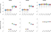 |
Fig. 1 Whiskers showing the median (grey, horizontal line) and dispersion of estimated parameters around the true value and of their standard error over 100 catalogs in three categories by the various estimation methods L1 DU, L1 DW, L2 EL1, L2 IL2, L2 555, CM 82, and CM128. The box limits are the first and third quartiles; the extreme horizontal bars indicate the fifth and 95th percentiles. |
3 Test on simulated catalogs
The robustness of the results from the possible inversion methods and, in particular, resistance to outliers was tested on a set of 300 simulated catalogs derived as follows. We first constructed a catalog by taking the ICRF3 at X-band (4536 sources) and applying a 16-parameter transformation with known values of the parameters to radio source coordinates. For this test, we chose the parameter values listed in the first column of Table 13 of Charlot et al. (2020) expressing the deformations between the ICRF3 and the ICRF2. This 16-parameter vector is noted as P0, and the “deformed” ICRF3 is designated as ICRF3D.
Then we constructed three groups consisting of 100 catalogs designated as ICRF3D1, ICRF3D2, and ICRF3D3. The three groups were constructed as follows: (i) 100 ICRF3D1 catalogs were computed from the ICRF3D catalog by introducing normally distributed position offsets with a standard deviation of 10 mas for 1000 randomly selected sources; (ii) 100 ICRF3D2 catalogs were computed similarly to ICRF3D1 catalogs except that the same position offset was introduced for 3000 randomly selected sources; and (iii) 100 ICRF3D3 catalogs were computed by introducing normally distributed position offsets with a standard deviation of 0.2 mas for all ICRF3D sources.
For each catalog, we adjusted the deformation parameters between the simulated catalog and the ICRF3 through the coordinate difference that reflected both the introduced deformation and the differences due to outliers. We used the ICRF3 errors to weight observation equations. For each source, the error of the coordinate difference is the quadratic sum of the error in each catalog. In this particular test case, errors are the same in both starting and simulated catalogs.
For each of the three categories of simulated catalogs, we obtained 100 vectors P of 16 parameters each. Their absolute differences to the true values  are represented by 1600 values of which whisker plots are shown in Fig. 1. In the same figure are the whiskers of the parameter formal errors. The median values of the absolute differences to P0 and of the parameter formal errors are reported in Table 1 together with the median number of outliers caught by the L2 EL1, L2 IL2, and L2 555 methods.
This test on synthetic data provided several insights. First, considering the estimated values, both pure L1 methods gave values of the parameters close to the true values with a high precision (differences of less than 0.001 µas). The L2 EL1 method as well as the L2 IL 2 method produced similarly satisfactory results. Thus, an L2 minimization is efficient if outliers have been preliminarily detected either with an L1 or an iterative L2 method. A hybrid L2 EL1 scheme accumulates the advantages of both L1 and L2 methods. The L1 outlier detection is efficient for catching all outliers, but L1 minimization can be problematic in terms of uniqueness of the solution. However, the implementation of the least-squares method is simple, produces the covariance of adjusted parameters, and therefore allows for straightforward computation of formal errors on parameters, and the solution is unique. Nevertheless, because it requires an L1 minimization in its first stage, the L2 EL1 scheme remains relatively computationally costly and could become problematic if it were applied to large data set of several billion objects. The L2 IL2 method that performs similarly in our simulations appears to be a good compromise. Finally, CM produces results with larger departures from the true value, but these departures are still less than 1 µas and are even more satisfactory when using 128 cells instead of 82 cells.
Secondly, regarding standard errors, CM provides error bars that tend to be smaller than L2 555. The introduced outliers are nearly all automatically rejected by the median applied in the CM method. The standard errors given by L2 EL1 and L2 IL2 in the first two tested categories appear unrealistically small and should likely be taken with some care.
Thirdly, from the outlier-catching point of view, the L2 EL1, L2 IL2, and L2 555 methods demonstrate comparable efficiency in performance. They all catch about 90% of the introduced outliers in the case where 1000 outliers were introduced. We note that a part of these introduced outliers was not detected due to their random-based generation. Some of the outliers fall close to the mean and, in fact, have no reason to be considered outliers. The detection percentage decreased if the number of outliers was raised to 3000 (~73% detection rate). In the case of a Gaussian noise, one cannot properly speak of outliers, and in fact, L2 EL1, L2 IL2, and L2 555 did not return consistent detection. L2 EL1 and L2 IL2, which act after a first removal of systematics, did not tag any outliers, as expected. L2 555, which acts before removal of systematics, likely considered the crest of the systematics as possible outliers, which is incorrect and dangerous.
Median values of absolute differences between estimated parameters P and true values P0, parameter standard errors, and number of detected outliers.
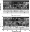 |
Fig. 2 Sky distribution of sources in common for six VLBI catalogs over cells of an equal-area SREAG grid (Malkin 2019) for 82 (top) and 128 (bottom) cells with the number of sources fallen into each cell. |
4 Test on real catalogs
After the above tests on simulated data, we conducted a comparison of various real catalogs made available in 2021 by individual analysis centers of the International VLBI Service for Geodesy and Astrometry (IVS; Nothnagel et al. 2017) against the ICRF3. These catalogs were obtained from state-of-the-art processing of geodetic VLBI data available since 1979. We used the VLBI solutions asi2021a (ASI; from the Italian Space Agency), aus2021a (AUS; Geoscience Australia), bkg2021a (BKG; Bundesamt für Kartographie und Geodäsie, Germany), opa2021a (OPA; Paris Observatory, France), usn2022a (USN; United States Naval Observatory), and vie2021a (VIE; Vienna University of Technology, Austria). An explanation and analysis of the differences between the catalogs are beyond the scope of this study and would deal with the analysis configurations, lists of sessions, and software packages used by each analyst. Further details can be found in the technical descriptions of the solutions available at the IVS data center. For our purpose, catalogs (including the ICRF3) were reduced to their common set of sources, that is the 4024 sources whose sky distribution is presented in Fig. 2.
In addition to the individual catalogs, we also included an average catalog computed as follows. Let xi, i = 1,…,n represents two-component vectors of source positions in n catalogs
 (4)
(4)
and Qi are covariance matrices of xi
 (5)
(5)
where  is the error in right ascension multiplied by cos δi,
  is the error in declination, and ρ(α, δ) is the correlation between αi and δi Then, average source position x is
 (6)
(6)
with covariance matrix of average position
 (7)
(7)
For each individual catalog, the 16 parameters of the transformation to ICRF3 were estimated by applying L1 DU, L1 DW, L2 EL1, L2 IL2, L2 555, and the CM method to a sphere divided into 82 cells and then 128 cells of equal area. The deformation parameters obtained with all methods for each catalog are shown in Fig. 3. Figure 4 displays the differences between the parameter values obtained from each method and those obtained more synthetically with the L2 555 method. The figure shows the averaging over the parameters or over the catalogs. In each case, the error bars are computed as the error on the mean (ratio of the standard deviation to the square root of the number of parameters or catalogs). For the catalogs, the parameter estimates obtained with each method appeared consistently within their error bars. The only small exception was AUS, whose results for L1 DU, CM 82, and CM 128 differed by about 2 µas (i.e., a poorly statistically significant value regarding the positional error of the radio sources and the order of the error bars on deformation parameters). The L1 DU and the CM methods diverged from other methods by about 2σ or more for several parameters. Nevertheless, the absolute values of these divergences were a few µas and have to be compared with the effective value of the parameters that, as can be seen in Fig. 3, are generally several tens of µas. Table 2 reports the mean and median absolute differences of L2 555 results computed across the parameters and the catalogs together with the mean and median uncertainty over all parameters and catalogs for each method, emphasizing conservative uncertainties for the CM methods, which are larger by a factor of two with respect to other methods but still within a few µas.
The number of outliers caught by the L2 555, L2 EL1, and L2 IL2 methods as well as the number of common outliers (intersection) is reported in Table 3. The number of outliers identified by the L2 EL1 and L2 IL2 methods is up to six times larger than the number caught by L2 555. Generally, the L2 EL1 and L2 IL2 detected almost all the outliers caught by L2 555 but not always (e.g., OPA). Reasons for this discrepancy could be due to the fact that the offset and error distribution in real catalog comparisons is not as simple as the one in the synthetic test. Though the simulated outlier distances were Gaussianly distributed around zero, most of the real catalogs showed distributions of distances containing both outliers close to zero, whose distribution can be assimilated to a Gaussian one, and tails with larger distances often not accounted for by the error and strongly departing from a normal distribution. Nevertheless, if the L2 EL1 and L2 IL2 methods detect substantially more outliers than L2 555, a major part of them (about two-thirds to three-quarters) are not critical and do not further influence the parameter adjustment significantly. The number of outliers caught by L2 EL1 and L2 IL2 is comparable, although their intersection is generally no more than 90%.
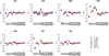 |
Fig. 3 Deformation parameters between catalogs and ICRF3 obtained by various methods. |
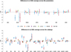 |
Fig. 4 Difference between deformation parameters obtained from various methods and their values obtained with L2 555 method averaged over the parameters (upper panel) or the catalogs (lower panel). |
Median values of absolute differences to L2 555 and of standard error computed across all catalogs and all parameters.
5 Conclusion
We compared several estimation methods based on L1 and L2 norms to detect the large-scale deformations between VLBI astrometric catalogs. We used simulated catalogs to investigate whether one method is more consistent with the known, a priori, truth than others. The methods that render the most correct results with a very low error, wiping out the largest number of outliers, are those based on an L1 minimization or the iterative L2 scheme (L2 IL2). The L2 555 and the CM methods both produce results consistent with the true parameter values within 1 µas, which is satisfactory regarding the standard error of the parameters and more global error budget quantities, such as axes stability (several tens of µas following Fey et al. 2015; Charlot et al. 2020). We used real VLBI catalogs to compare the results given by each method and found that all were consistent within a few µas. The results obtained with direct L1 minimization as well as the hybrid L2 EL1 scheme and the iterative L2 IL2 method are the most consistent with the results obtained using L2 555 (after rejection of outliers).
As to the CM method, the comparisons in Sects. 3 and 4 show that the variantwith 128 cells gives estimates mostly closer to the orientation parameters and provides better precision of the parameters than the variant with 82 cells. Though the simulation suggests that L1-based methods possibly converge in a more straightforward manner toward the correct values of the parameters, they are more difficult to implement in terms of programming and computational cost, which is not critical for catalogs of a few thousand sources but could become very critical for catalogs of millions of objects or more. Moreover, the derivation of standard errors on parameters – which is straightforward from residuals and covariance in L2 – as well as the handling of weights was not implemented in the L1 routines that we used.
In the future, such methodologies could be extended to larger catalogs and higher VSH degrees in order to model smaller-scale differences arising from systematics, real effects in source positions, or apparent velocities. In particular, the value of estimated parameters and the sensitivity of the method to outliers and deformations could depend on the number of estimated parameters (Mignard et al. 2018).
Number of outliers detected by L2 555, L2 EL1, and L2 IL2 and number of common outliers.
Acknowledgements
Constructive comments and useful suggestions from an anonymous reviewer are gratefully acknowledged. The radio source position catalogs used for this study was obtained from the International VLBI Service for geodesy and astrometry (IVS) thanks to the regular collaboration of several institutes to this organism operating geodetic VLBI: Agenzia Spaziale Italiana (Italy), Geoscience Australia (Australia), Bundesamt für Kartographie und Geodäsie (Germany), Observatoire de Paris – Paris Sciences et Lettres (France), United States Naval Observatory (USA), and Technische Universität Wien (Austria).
References
- Amiri-Simkooei, A. 2003, J. Surveying Eng., 129, 37 [CrossRef] [Google Scholar]
- Andersen, R. 2008, Modern Methods for Robust Regression (USA: Sage), 152 [Google Scholar]
- Arias, E. F., & Bouquillon, S. 2004, A&A, 422, 1105 [NASA ADS] [CrossRef] [EDP Sciences] [Google Scholar]
- Arias, E. F., Charlot, P., Feissel, M., & Lestrade, J.-F. 1995, A&A, 303, 604 [Google Scholar]
- Brown, A. G. A., Vallenari, A., Prusti, T., et al. 2021, A&A, 649, A1 [NASA ADS] [CrossRef] [EDP Sciences] [Google Scholar]
- Charlot, P., Jacobs, C. S., Gordon, D., et al. 2020, A&A, 644, A159 [EDP Sciences] [Google Scholar]
- Feissel, M., & Mignard, F. 1998, A&A, 331, L33 [Google Scholar]
- Fey, A. L., Gordon, D., Jacobs, C. S., et al. 2015, AJ, 150, 58 [Google Scholar]
- Gaia Collaboration (Klioner, S. A., et al.) 2021, A&A, 649, A9 [EDP Sciences] [Google Scholar]
- Gaia Collaboration (Klioner, S. A., et al.) 2022, A&A, 667, A148 [NASA ADS] [CrossRef] [EDP Sciences] [Google Scholar]
- Gontier, A.-M., Le Bail, K., Feissel, M., & Eubanks, T. M. 2001, A&A, 375, 661 [NASA ADS] [CrossRef] [EDP Sciences] [Google Scholar]
- Kareinen, N., Hobiger, T., & Haas, R. 2016, J. Geodyn., 102, 39 [NASA ADS] [CrossRef] [Google Scholar]
- Koch, K.-R. 1999, Parameter Estimation and Hypothesis Testing in Linear Models (Berlin: Springer Science & Business Media) [CrossRef] [Google Scholar]
- Lambert, S. 2014, A&A, 570, A108 [NASA ADS] [CrossRef] [EDP Sciences] [Google Scholar]
- Liu, N., Lambert, S. B., Zhu, Z., & Liu, J. C. 2020, A&A, 634, A28 [EDP Sciences] [Google Scholar]
- Liu, N., Lambert, S., Charlot, P., et al. 2021, A&A, 652, A87 [NASA ADS] [CrossRef] [EDP Sciences] [Google Scholar]
- Makarov, V. V. 2022, AJ, 164, 157 [NASA ADS] [CrossRef] [Google Scholar]
- Malkin, Z. 2019, AJ, 158, 158 [NASA ADS] [CrossRef] [Google Scholar]
- Malkin, Z. 2021, MNRAS, 506, 5540 [NASA ADS] [CrossRef] [Google Scholar]
- Malkin, Z. 2022, Astron. Rep., 66, 778 [NASA ADS] [CrossRef] [Google Scholar]
- Matt, J. 2022, Constrained minimum L1-norm solutions of linear equations, MATLAB Central File Exchange [Google Scholar]
- Mignard, F., & Klioner, S. 2012, A&A, 547, A59 [NASA ADS] [CrossRef] [EDP Sciences] [Google Scholar]
- Mignard, F., Klioner, S. A., Lindegren, L., et al. 2018, A&A, 616, A14 [NASA ADS] [CrossRef] [EDP Sciences] [Google Scholar]
- Nothnagel, A., Artz, T., Behrend, D., & Malkin, Z. 2017, J. Geodesy, 91, 711 [NASA ADS] [CrossRef] [Google Scholar]
- Press, W. H., Teukolsky, S. A., Vetterling, W. T., & Flannery, B. P. 2002, Numerical Recipes in C++ : the Art of Scientific Computing (Cambridge: Cambridge University Press) [Google Scholar]
- Prusti, T., de Bruijne, J. H. J., Brown, A. G. A., et al. 2016, A&A, 595, A1 [NASA ADS] [CrossRef] [EDP Sciences] [Google Scholar]
- Sokolova, Ju., & Malkin, Z. 2007, A&A, 474, 665 [NASA ADS] [CrossRef] [EDP Sciences] [Google Scholar]
All Tables
Median values of absolute differences between estimated parameters P and true values P0, parameter standard errors, and number of detected outliers.
Median values of absolute differences to L2 555 and of standard error computed across all catalogs and all parameters.
Number of outliers detected by L2 555, L2 EL1, and L2 IL2 and number of common outliers.
All Figures
|
Fig. 1 Whiskers showing the median (grey, horizontal line) and dispersion of estimated parameters around the true value and of their standard error over 100 catalogs in three categories by the various estimation methods L1 DU, L1 DW, L2 EL1, L2 IL2, L2 555, CM 82, and CM128. The box limits are the first and third quartiles; the extreme horizontal bars indicate the fifth and 95th percentiles. |
| In the text | |
|
Fig. 2 Sky distribution of sources in common for six VLBI catalogs over cells of an equal-area SREAG grid (Malkin 2019) for 82 (top) and 128 (bottom) cells with the number of sources fallen into each cell. |
| In the text | |
|
Fig. 3 Deformation parameters between catalogs and ICRF3 obtained by various methods. |
| In the text | |
|
Fig. 4 Difference between deformation parameters obtained from various methods and their values obtained with L2 555 method averaged over the parameters (upper panel) or the catalogs (lower panel). |
| In the text | |
Current usage metrics show cumulative count of Article Views (full-text article views including HTML views, PDF and ePub downloads, according to the available data) and Abstracts Views on Vision4Press platform.
Data correspond to usage on the plateform after 2015. The current usage metrics is available 48-96 hours after online publication and is updated daily on week days.
Initial download of the metrics may take a while.