| Issue |
A&A
Volume 689, September 2024
|
|
|---|---|---|
| Article Number | A97 | |
| Number of page(s) | 6 | |
| Section | Planets and planetary systems | |
| DOI | https://doi.org/10.1051/0004-6361/202244087 | |
| Published online | 05 September 2024 | |
Exocomet orbital distribution around β Pictoris
Max-Planck-Institut für Sonnensystemforschung,
Justus-von-Liebig-Weg 3,
37077
Göttingen,
Germany
Received:
23
May
2022
Accepted:
30
July
2024
The ~23 Myr young star β Pictoris (β Pic) is a laboratory for planet formation studies because of its observed debris disk, its directly imaged super-Jovian planets β Pic b and c, and the evidence of extrasolar comets that regularly transit in front of the star. The most recent evidence of exocometary transits around β Pic came from stellar photometric time series obtained with the TESS space mission. Previous analyses of these transits constrained the orbital distribution of the underlying exocomet population to a range between about 0.03 and 1.3 AU assuming a fixed transit impact parameter. We examine the distribution of the observed transit durations (Δt) to infer the orbital surface density distribution (δ) of the underlying exocomet sample. The effect of the geometric transit probability for circular orbits was properly taken into account, but we assumed that the radius of the transiting comets and their possible clouds of evaporating material are much smaller than the stellar radius. We show that a narrow belt of exocomets around β Pic, in which the transit impact parameters are randomized but the orbital semimajor axes are equal, results in a pile-up of long transit durations. This is in contrast to observations, which reveal a pile-up of short transit durations (Δt ≈ 0.1 d) and a tail of only a few transits with Δt > 0.4 d. A flat density distribution of exocomets between about 0.03 and 2.5 AU results in a better match between the resulting Δt distribution and the observations, but the slope of the predicted Δt histogram is not sufficiently steep. An even better match to the observations can be produced with a δ ∝ aβ power law. Our modeling reveals a best fit between the observed and predicted Δt distribution for β = −0.15−0.10+0.05. A more reasonable scenario in which the exocometary trajectories are modeled as hyperbolic orbits can also reproduce the observed Δt distribution to some extent. Future studies might reproduce the observed Δt distribution with a full exploration of the four-dimensional parameter space of highly eccentric orbits, and they might need to relax our assumption that the transiting objects are smaller than the stellar disk. The number of observed exocometary transits around β Pic is currently too small to validate the previously reported distinction of two distinct exocomet families, but this might be possible with future TESS observations of this star. Our results nevertheless imply that cometary material exists on highly eccentric orbits with a more extended range of semimajor axes than suggested by previous spectroscopic observations.
Key words: methods: data analysis / techniques: photometric / occultations / comets: general / planets and satellites: detection
© The Authors 2024
 Open Access article, published by EDP Sciences, under the terms of the Creative Commons Attribution License (https://creativecommons.org/licenses/by/4.0), which permits unrestricted use, distribution, and reproduction in any medium, provided the original work is properly cited.
This article is published in open access under the Subscribe to Open model.
Open Access funding provided by Max Planck Society.
1 Introduction
The star β Pictoris (β Pic) has become one of the few benchmark systems for studies of planet formation, in which a debris disk (Smith & Terrile 1984), extrasolar comets Ferlet et al. (1987); Beust et al. (1990); Kiefer et al. (2014), and even two extrasolar giant planets (β Pic b Lagrange et al. 2009, 2010 and c Lagrange et al. 2019; Nowak et al. 2020) have been found. It is a naked-eye (mV = 3.86) A-type star on the zero-age main sequence. Its parallax measurement of 50.903 (± 0.1482) milliarcseconds from Gaia Early Data Release 3 (Gaia Collaboration 2016, 2021) suggests a distance of ![$\[19.6345_{-0.0569}^{+0.0573} ~\mathrm{pc}\]$](/articles/aa/full_html/2024/09/aa44087-22/aa44087-22-eq2.png) . As part of a comoving group of stars, the age of β Pic has become exceptionally well constrained. Isochronal fitting of a total of 30 A-, F, and G-type stars from the β Pic moving group suggest an age of 23 (±3) Myr (Mamajek & Bell 2014), and more recent dynamical age estimates based on Gaia DR2 yield
. As part of a comoving group of stars, the age of β Pic has become exceptionally well constrained. Isochronal fitting of a total of 30 A-, F, and G-type stars from the β Pic moving group suggest an age of 23 (±3) Myr (Mamajek & Bell 2014), and more recent dynamical age estimates based on Gaia DR2 yield ![$\[18.5_{-2.4}^{+2.0}\]$](/articles/aa/full_html/2024/09/aa44087-22/aa44087-22-eq3.png) Myr (Miret-Roig et al. 2020).
Myr (Miret-Roig et al. 2020).
The detection and characterization of exocomets around β Pic has an exceptionally long history, with an initial discovery preceding the detection of the first exoplanets by almost a decade. First indications of exocomets came from variations in the Ca II-K absorption line profile of β Pic that was interpreted as evidence of infalling cometary material on the star (Ferlet et al. 1987; Beust et al. 1990). More recent high-resolution stellar spectroscopy distinguished two families of comets located at 10(± 3) Rs and 19(± 4) Rs Kiefer et al. (2014), respectively, where Rs is the stellar radius.
In addition to indications from spectroscopy, variations in the apparent brightness of β Pic have been noted in ground-based archival data from La Silla by the Geneva Observatory. A peculiar dimming event around 10 November 1981, which took several days, has been interpreted as the passage of a planet, a group of planets, or planetesimals with a total cross-section area comparable to that of Jupiter (Lecavelier Des Etangs et al. 1995). Recent follow-up observations of β Pic during the transit of the outer regions of the Hill sphere of its giant exoplanet β Pic b did not reveal any new dimming events, however (Kenworthy et al. 2021). Modern space-based stellar photometry of β Pic from the ongoing TESS mission led to the discovery of three cometary transits (Zieba et al. 2019), a phenomenon that had been anticipated long ago (Lecavelier Des Etangs et al. 1999). These three events, observed in TESS sectors 4–7 from 19 October 2018 to 1 February 2019, were monitored with a much better time resolution than the historical data. The TESS 2-minute short cadence of β Pic is key to characterizing the transit duration of exocometary events presented in this report.
More recently, Lecavelier des Etangs et al. (2022, hereafter L+22) analyzed additional TESS observations of β Pic in sectors 31–34 from 20 November 2020 to 8 February 2021. Some of these transits were also reported by Pavlenko et al. (2022). In their combined analyses of the entire TESS data of β Pic, L+22 found 30 cometary transits, including the three that were known previously. Their analysis also revealed a striking similarity between the cumulative size distribution of the comets around β Pic to the cometary size distribution observed in the Solar System. Both distributions are consistent with the canonical size distribution first derived by Dohnanyi (1969) for a collisionally relaxed population.
In addition to cometary studies around β Pic, analyses of space-based photometry of the Kepler mission showed evidence of cometary transits around other early-type stars, such as KIC 3542116 (Rappaport et al. 2018) and KIC 8462852 (Boyajian et al. 2016; Wyatt et al. 2018). These recent results show that the community is currently transitioning from an era of exocometary transit detections to an era of exocomet characterization.
Using the distribution of the observed exocomet transit times around β Pic, we attempt such a characterization in this study. L+22 estimated that the periastron distances range between 0.03 AU and 1.3 AU around β Pic. Their calculations assumed that each comet transits the star across the entire stellar diameter. We extend the analysis of the orbital distribution of these exocomets by investigating the histogram of the transit duration variations for random transit impact parameters and taking the transit probability as a function of the distance to the star into account. First, we investigate extended cometary rings around β Pic. Because comets are unlikely to survive evaporation at distances ≲1 AU for very long, however, we also investigate comets on highly eccentric (e~1) hyperbolic orbits.
2 Methods
An important assumption throughout this study is that the radii of the transiting comets are smaller than the stellar radius. This assumption is justified by the observed transit durations, as we demonstrate in Sect. 3.5.
2.1 Circular orbits
For the purpose of illustration, we first considered a star that is transited by a sample of exocomets on circular orbits with randomized transit impact parameters (b). Figure 1a displays the resulting transit paths with a length of
![$\[p=2 R_{\mathrm{s}} \sqrt{1-b^2}.\]$](/articles/aa/full_html/2024/09/aa44087-22/aa44087-22-eq4.png) (1)
(1)
When all these objects are arranged in a narrow ring around the star with essentially the same orbital semimajor axis (a) but slightly different orbital inclinations with respect to the line of sight (i), then they will all have the same orbital velocity, but exhibit different transit durations (Δt) depending on their respective transit impact parameter. The resulting histogram of this hypothetical narrow-ring exocomet population is shown in Fig. 1b, which shows a pile-up towards high values of Δt. As a consequence, the shortest transit durations can be expected to be rare if the Δt distribution were caused by a comet sample with similar orbital distances.
In β Pic, however, this is not the case. Inspection of the Δt values measured by L+22 (extended data Table 2 therein) shows the exact opposite, namely a Δt pile-up toward low values. When the measurements of L+22 are counted in bins with a width of 0.1 d, we obtain the histogram shown in Fig. 2. It is important to note that the lack of objects with long durations is not due to a sensitivity bias that would favor short transit durations. Quite the contrary, the transit detectability increases with transit duration.
Examination of the L+22 data reveals that 15 transits lie within [0.1d, 0.2d], and 5 of them have the lowest value of Δt = 0.10d, and only one transit in each of the Δt intervals [0.4d, 0.5d], [0.5d, 0.6d], and [0.6d, 0.7d], respectively. The 5 short-duration transits are very likely not near-grazing transits because near-grazing transits are expected to be very rare (when i has a flat prior and is randomly distributed) (see Fig. 1). Instead, at least some of them are very likely to have transit impact parameters near zero. As a consequence, they should also have the shortest orbital period.
In the limit of circular orbits and under the assumption that the radius of the comets and any possible clouds of evaporating material are much smaller than the stellar radius, the transit duration is given as the transit path divided by the orbital velocity,
![$\[\Delta t=\frac{2 R_{\mathrm{s}} \sqrt{1-b^2}}{v},\]$](/articles/aa/full_html/2024/09/aa44087-22/aa44087-22-eq5.png) (2)
(2)
where the orbital velocity is given as
![$\[v=\frac{2 \pi a}{P},\]$](/articles/aa/full_html/2024/09/aa44087-22/aa44087-22-eq6.png) (3)
(3)
and P is the orbital period. Together with an approximation for Kepler’s third law, in which the cometary mass is vanishingly low compared to the stellar mass,
![$\[P \sim 2 \pi \sqrt{\frac{a^3}{G M_{\mathrm{s}}}},\]$](/articles/aa/full_html/2024/09/aa44087-22/aa44087-22-eq7.png) (4)
(4)
and where G is the gravitational constant, we find
![$\[\Delta t=2 R_{\mathrm{s}} \sqrt{\frac{a\left(1-b^2\right)}{G M_{\mathrm{s}}}}\]$](/articles/aa/full_html/2024/09/aa44087-22/aa44087-22-eq8.png) (5)
(5)
![$\[a=\frac{G M_{\mathrm{s}}}{\left(1-b^2\right)}\left(\frac{\Delta t}{2 R_{\mathrm{s}}}\right)^2,\]$](/articles/aa/full_html/2024/09/aa44087-22/aa44087-22-eq9.png)
where the transit impact parameter is
![$\[b=\frac{a}{R_{\mathrm{s}}} \tan \left(\frac{\pi}{2}-i\right).\]$](/articles/aa/full_html/2024/09/aa44087-22/aa44087-22-eq10.png) (7)
(7)
The geometrical transit probability (![$\[\mathcal{P}\]$](/articles/aa/full_html/2024/09/aa44087-22/aa44087-22-eq11.png) ) favors the transits of objects in close orbits. Generally speaking, for an object that is much smaller than its host star,
) favors the transits of objects in close orbits. Generally speaking, for an object that is much smaller than its host star, ![$\[\mathcal{P}\]$](/articles/aa/full_html/2024/09/aa44087-22/aa44087-22-eq12.png) = Rs/a. For reference, a planet at 1 AU around a Sun-like star has a geometric transit probability of about 0.5%. In our simulations, this selection effect is taken into account by randomizing the orbital inclination of the exocomets at their respective orbital distances to the star and by counting only objects with transit impact parameters b ≤ 1. Strictly speaking, it is really the probability density of cos(i) that is uniform. Our randomization of 0° ≤ i ≤ 90° is still justified, however, because transits only occur for inclinations near 90°, where i and cos(i) converge.
= Rs/a. For reference, a planet at 1 AU around a Sun-like star has a geometric transit probability of about 0.5%. In our simulations, this selection effect is taken into account by randomizing the orbital inclination of the exocomets at their respective orbital distances to the star and by counting only objects with transit impact parameters b ≤ 1. Strictly speaking, it is really the probability density of cos(i) that is uniform. Our randomization of 0° ≤ i ≤ 90° is still justified, however, because transits only occur for inclinations near 90°, where i and cos(i) converge.
By randomizing the orbital inclinations in Eq. (7) and assuming a distribution of exocometary orbits around β Pic, we can then predict an observed distribution for Δt and compare this prediction with the data of L+22 compiled in Fig. 2.
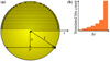 |
Fig. 1 Pile-up of long transit paths (and long transit durations, Δt) for randomly distributed transit impact parameters. |
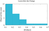 |
Fig. 2 Transit durations of 30 exocometary events around β Pic as observed by L+22 using TESS data. |
2.2 Hyperbolic orbits
While previous studies concluded that the observed transiting comets around β Pic have periastron distances near 0.1 AU, comets are not expected to be long-lived at such close-in separations from this A5 star for extended periods. Hence, the assumption of circular orbits is likely an oversimplification of the situation. Moreover, spectral absorption features of the cometary coma have shown in-transit acceleration, which strongly suggests significant orbital eccentricities (Kennedy 2018). This also agrees with the orbital eccentricities of the Solar System comets, which often have e~1.
We therefore also explored the Δt histograms for comets on hyperbolic orbits. Our nomenclature is illustrated together with a reference trajectory in Fig. 3, where ![$\[\vec{r}\]$](/articles/aa/full_html/2024/09/aa44087-22/aa44087-22-eq13.png) is the radius vector of the comet,
is the radius vector of the comet, ![$\[\vec{v}\]$](/articles/aa/full_html/2024/09/aa44087-22/aa44087-22-eq14.png) is the orbital velocity vector, ϕ is the angle between
is the orbital velocity vector, ϕ is the angle between ![$\[\vec{v}\]$](/articles/aa/full_html/2024/09/aa44087-22/aa44087-22-eq15.png) and the line perpendicular to
and the line perpendicular to ![$\[\vec{r}\]$](/articles/aa/full_html/2024/09/aa44087-22/aa44087-22-eq16.png) , and θ is the angle between the orientation of the periastron and our line of sight. The velocity component perpendicular to the line of sight is relevant to our transit studies. We refer to it as in-transit velocity (υt).
, and θ is the angle between the orientation of the periastron and our line of sight. The velocity component perpendicular to the line of sight is relevant to our transit studies. We refer to it as in-transit velocity (υt).
Our investigation of hyperbolic orbits has four free parameters, that is, a, e, θ, and i. For any choice of a, e, and θ, we computed
![$\[\phi=\arctan \left(\frac{e \sin (\theta)}{1+e \cos (\theta)}\right),\]$](/articles/aa/full_html/2024/09/aa44087-22/aa44087-22-eq17.png) (8)
(8)
![$\[r=\frac{a\left(e^2-1\right)}{1+e \cos (\theta)},\]$](/articles/aa/full_html/2024/09/aa44087-22/aa44087-22-eq18.png) (9)
(9)
![$\[v=\sqrt{G M_{\mathrm{s}}\left(\frac{2}{r}-\frac{1}{a}\right)},\]$](/articles/aa/full_html/2024/09/aa44087-22/aa44087-22-eq19.png) (10)
(10)
to finally obtain the in-transit velocity as υt = υcos(ϕ), which we assumed to be constant. The transit duration then follows from Eq. (2), but using υt instead of υ, and with b as computed with Eq. (7) for any given choice of a and i. For hyperbolic orbits, we used the convention of a < 0 to make Eqs. (8)–(10) applicable.
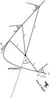 |
Fig. 3 Parameterization of hyperbolic orbits. |
3 Results
For β Pic, we assumed the best-fit radius of Rs = 1.497 R⊙ and a mass of Ms = 1.797 M⊙ (the subscript ⊙ refers to solar values) according to some of the most recent and well-constrained estimates using asteroseismology (Zwintz et al. 2019). For the most short-duration transit events with Δt = 0.1 d and b = 0, Eq. (6) for circular orbits then yields a = 0.026 AU. This agrees with the estimated periastron distance of 0.03 AU by L+22, although the authors used slightly different stellar mass and radius and a fixed mean transit path of ![$\[\bar{p}=\pi R_{\mathrm{s}} / 2\]$](/articles/aa/full_html/2024/09/aa44087-22/aa44087-22-eq20.png) . Taking
. Taking ![$\[\bar{p}=2 R_{\mathrm{s}} \sqrt{1-\bar{b}^2}\]$](/articles/aa/full_html/2024/09/aa44087-22/aa44087-22-eq21.png) in Eq. (1), this is equivalent to a mean transit impact parameter of
in Eq. (1), this is equivalent to a mean transit impact parameter of ![$\[\bar{b} \approx 0.619\]$](/articles/aa/full_html/2024/09/aa44087-22/aa44087-22-eq22.png) .
.
Comets in close-in orbits around β Pic like this, however, can hardly withstand evaporation for more than a few orbits. Circular orbits are therefore certainly an oversimplification of the real situation. Nevertheless, because of their geometric simplicity, circular orbits are quite helpful for a better understanding of how different orbital distributions of the comets translate into different Δt diagrams. Hence, we first explored several scenarios with circular orbits for didactic purposes, although the actual distribution of cometary trajectories around β Pic certainly looks different.
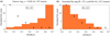 |
Fig. 4 Histogram of the transit durations (Eq. (5)) based on 300 000 randomly chosen orbital orientations of an exocometary sample. The black dots illustrate the bin counts compiled from L+22. (a) Orbital distance fixed to 2.5 AU around β Pic. (b) Orbital distance drawn from a flat distribution with 0.026 AU ≤ a ≤ 2.5 AU around β Pic. The histograms are normalized to 15, corresponding to Fig. 2. |
3.1 Narrow ring
First, we executed simulations for a sample of exocomets at a fixed orbital distance. In this setup, the comet surface density (δ) as a function of a was zero everywhere except for an arbitrary distance a′. The exact value of a′ is irrelevant at this point because the shape of the resulting Δt distribution only depends on the distribution of the transit impact parameters (Fig. 1) and the normalization depends on the unknown occurrence rate of exocomet transits around β Pic. Moreover, as we show below, the shape of the histogram does not fit the observations in the first place.
We therefore took an arbitrary value of a′ = 2.5 AU and produced 300000 random draws1 of the orbital inclination in the interval 0° ≤ i ≤ 90°, the result of which is shown in Fig. 4a. For better comparability to Fig. 2, the histogram was normalized to 15 along the ordinate, and the central values of the exocomet histogram from L+22 were added as black points. The total number of transits among the 300 000 realizations is 587, or 0.20%.
Most importantly, and most obviously, the distribution in Fig. 4a shows a pile-up toward high values of Δt and a lack of short transit durations. This is opposite to the histogram for the exocomets around β Pic (Fig. 2). Since the test objects in this simulation all have the same orbital semimajor axis, the shape of the histogram is entirely determined by the distribution of the transit impact parameters, as described in Fig. 1. This discrepancy is not due an observational bias caused by the dependence of the geometric transit probability on the orbital semimajor axis. As a result, the stark discrepancy of the resulting distribution in Fig. 4a compared to the observations of L+22 (Fig. 2) clearly shows that the Δt distribution observed around β Pic cannot be explained by a narrow ring of comets at a given orbital distance with equally distributed transit impact parameters.
3.2 Extended flat ring
We also investigated an expanded ring of exocomets with a flat density distribution (δ ∝ a0 = const.) between 0.026 AU, corresponding to an innermost orbit that is compatible with the observed minimum transit duration around β Pic, and 2.5 AU. Initial tests showed that orbits beyond 2.5 AU do not produce significant numbers of transiting objects, and we therefore chose this orbit as an outer boundary. The reason for this low rate of transits in wide orbits is the geometric transit probability, which scales as ∝ a−1.
The resulting Δt histogram is shown in Fig. 4b. The total number of transits among the 300000 realizations is 2513, a fraction of 0.84%. The key distinction with respect to the narrow-ring scenario in Fig. 4a is the pile-up toward short transit durations, which agrees far better with the observations. With the histogram normalized to 15 transits in the [0.1 d, 0.2 d] bin, the extended flat ring scenario predicts a significant overabundance of transits for 0.2 d < Δt < 0.6 d. This suggests that in order to reproduce the observed Δt distribution with circular orbits, the comet density of a hypothetical ring around β Pic would need to decline with distance, which is what we explore in the following.
3.3 Power-law ring
Next, we investigated an inner ring boundary of 0.026 AU (to reproduce the observed minimum transit durations with circular orbits) with an exocomet density decline as per the power law δ ~ a−β. As an initial test, we studied a δ ∝ a−1 power-law ring, the resulting histogram of which is presented in Fig. 5a. The total number of transits among the 300 000 realizations is 11494, corresponding to 3.83%. When normalized to 15 transits in the [0.1 d, 0.2 d] bin, the theoretical distribution underestimates the observed transit bin counts around β Pic consistently for all of the longer transit durations. This result immediately shows that the exocomet density decline resulting from the initial guess of β = −1 is too steep.
To optimize our search for the best-fitting value of β, we tested a total of 40 power laws with −2 ≤ β ≤ −0.05 in steps of 0.05. For each test value of β, we performed 300 000 randomized realizations, in which the orbital semimajor axis was chosen from the respective power-law density and the transit geometry was drawn from a uniform distribution for 0° ≤ i ≤ 90°. This resulted in a total of 1.2 million computer-generated realizations. For each of the 40 power laws, we calculated the residual sum of squares, which we find to be minimal for β = −0.15. Moreover, we computed the standard deviation of the best-fitting β value from the χ2 distribution (Zhang et al. 1986; Heller et al. 2009) to obtain formal error bars, resulting in ![$\[\beta=-0.15_{-0.10}^{+0.05}\]$](/articles/aa/full_html/2024/09/aa44087-22/aa44087-22-eq23.png) .
.
The resulting best-fit Δt histogram for this δ ∝ a−0.15 power-law ring is presented in Fig. 5b. It includes 3064 transits generated from 300000 realization, corresponding to a transit fraction of 0.84%.
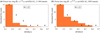 |
Fig. 5 Similar to Fig. 4, except that the orbital distances of the comets were drawn from different power-law distributions. (a) a−1 power law with an inner truncation radius at 0.026 AU around β Pic. (b) Best-fit a−0.15 power law with an inner truncation radius at 0.026 AU around β Pic. |
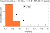 |
Fig. 6 Histogram of the transit durations (Eq. (5)) based on 300 000 randomly chosen orbital orientations of an exocometary sample on a hyperbolic orbit. The black dots illustrate the bin counts compiled from L+22. The orbital elements are given in the title. The histogram was normalized to 15 corresponding to Fig. 2. |
3.4 Hyperbolic orbits
Comets on circular orbits in extended flat rings or power-law rings are very useful for a sense of the parameter dependencies and their effect on the Δt histograms. We are ultimately interested in highly eccentric orbits, however, to create a physically plausible scenario. Comets will live longer on high-eccentricity orbits because most of the time is spent far from the star, and hence, eccentric orbits are more physically plausible for a system of a given age.
We tested different hyperbolic orbits with various combinations of a, e, and θ with a flat prior on i and still assuming negligible cometary radii with respect to the stellar diameter. We did not find a match of the resulting Δt distribution that was as good as we found for the power-law ring. One of the best matches is shown in Fig. 6, where a = −0.1 AU, e = 1.5, and θ = 88°. In this setup, the cometary material sweeps across the stellar disk as seen from Earth, when it is at a stellar distance of 0.12 AU. In comparison to the Δt histograms for circular orbits, however, we were unable to reproduce a tail as wide as in the Δt distribution. Parabolic orbits have the same problem of a relatively narrow Δt distribution, as shown in Fig. 6.
In Fig. 7, we illustrate the length of the star-comet radius vector (r) as a function of θ. The solid lines represent near-parabolic orbits with e = 1.01 for three choices of a ∈ {0.1, 0.2, 1.0} AU. For these near-parabolic orbits, most orientations of the periastron with respect to our line of sight indeed result in relatively close-in orbital radii during the observed transits.
In hyperbolic orbits, r is larger than in near-parabolic orbits for most values of θ (dashed lines for e = 1.2), where cometary material could withstand evaporation. However, hyperbolic orbits have the issue that these objects would be external to the β Pic system. Moreover, none of our hyperbolic trajectory simulations with randomized orbital inclinations yields a match to the observations that is as good as the δ ∝ a−0.15 power-law ring. Our tests were not exhaustive, however, and a much better fit might exist. More work is also needed to explore the parameter space for a distribution of semimajor axes with parabolic orbits because this might help in much the same way as for circular orbits.
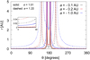 |
Fig. 7 Variation in the orbital radius as a function of the orientation of the line of sight for hyperbolic orbits. We show two different orbital eccentricities (e ∈ {1.01, 1.2}). |
3.5 Effect of the comet size
Our calculations show that the observed transit durations of about 0.1 d to 0.5 d can be adequately explained by cometary material with periastron distances between 0.026 AU and 0.12AU. In all these calculations, we assumed that the size of the comets is negligible for the transit duration.
If the observed transit durations were dominated by the extent of the transiting cometary material, then the time spent in transit would be much longer for any given instantaneous distance to the star. For a cloud of cometary material that has roughly the size of the star, for example, the transit duration would about double compared to our estimates with Eqs. (2) and (5).
In turn, in order to fit the theoretical transit duration of an extended cometary cloud with a radius similar to β Pic to the observed transits durations of about 0.1 d, the distance between the star and the comets would need to be about 0.006 AU, which is physically implausible because this distance is smaller than the size of the star.
Our results and interpretation agree with simulations by Lecavelier Des Etangs et al. (1999) for a cometary transit around β Pic. These authors found that even a cloud of opaque cometary material around an evaporating cometary core is significantly smaller than the star. Their simulated transit light curve for a comet at a nominal distance of 1 AU from the star (Lecavelier Des Etangs et al. 1999, Fig. 1 therein) illustrates that most of the stellar occultation is completed after 15 h to 20 h, corresponding to about 0.6 d to 0.8 d. With Eq. (5) we obtain 0.6 d.
4 Conclusions
Our analysis of the transit durations from a total of 30 exocometary transit events observed by L+22 suggests that the density of cometary material (δ) around β Pic can be reasonably well approximated by a power-law distribution δ ~ a−β with ![$\[\beta=-0.15_{-0.10}^{+0.05}\]$](/articles/aa/full_html/2024/09/aa44087-22/aa44087-22-eq24.png) under the assumption of circular orbits. This power law is derived from histograms of the exocometary transit durations that imply orbital separations of between 0.026 and about 2 AU from star, details depending on the unknown transit impact parameters of the individual transit events. The short lifetimes that can be expected for comets closer than about 1 AU from the star do not make this a very likely scenario, however. A very recent origin of the observed comet family or families around β Pic would then need to be claimed in that case.
under the assumption of circular orbits. This power law is derived from histograms of the exocometary transit durations that imply orbital separations of between 0.026 and about 2 AU from star, details depending on the unknown transit impact parameters of the individual transit events. The short lifetimes that can be expected for comets closer than about 1 AU from the star do not make this a very likely scenario, however. A very recent origin of the observed comet family or families around β Pic would then need to be claimed in that case.
A more plausible scenario involves comets on highly eccentric orbits, which we find could indeed lead to the observed transit durations of as short as about 0.1 d. Our predicted Δt histograms for a single family of comets on the same hyperbolic or near-parabolic orbit, however, cannot reproduce the observed transit times. We can also rule out that the cometary size is a dominant aspect, and this therefore means that either substantial fine-tuning of the orientation of a highly eccentric orbit is required or that a recent breakup of an eccentric comet into a cometary family matches the data only poorly. Considering that objects with similar orbits have long been used to explain the common redshift of spectroscopic features around β Pic Beust et al. (1990) and considering that a single comet family is a more natural model as it requires far fewer nontransiting objects than multiple families (Boyajian et al. 2016; Wyatt et al. 2018), our conclusion might be quite powerful because the method applied in this paper is simple.
Previous high-resolution stellar spectroscopy distinguished two families of comets located at 10 (± 3) Rs and 19 (± 4) Rs (Kiefer et al. 2014), corresponding to about 0.07 AU and 0.13 AU, respectively. The resulting transit durations would be about 0.16 d and 0.22 d and thus be unresolved in our histograms. Nevertheless, our new results suggest that these previously detected cometary families are but the inner compact regions of what could really be an extended stream of comets on hyperbolic orbits. In other words, our results imply the existence of highly eccentric cometary material with a more extended range of semimajor axes than might be expected based on the spectroscopic data alone.
Future photometric observations of exocometary transits around β Pic have the potential to further constrain the orbital distribution of comets around that star. In addition to the 30 transits analyzed in this report, there is the possibility that some very short (≲ 0.1 d) events at the limit of detectability could still be found in the available data. It is well possible that TESS will reobserve β Pic in the future, which might add several dozen additional transits. Key improvements on the data analysis side are possible if the transit impact parameters of individual events can be measured. This is challenging, however, because it depends on proper modeling of the stellar limb darkening, and β Pic might be too photometrically active for this type of fine-structure analysis.
A natural extension of this work would be a systematic search for a best-fitting solution of hyperbolic near-parabolic orbits that reproduce the Δt diagram inferred from L+22. This analysis might need to use a radially extended family of comets, as suggested by our best-fitting δ ∝ a−0.15 power-law ring solution. Finally, our assumption that the comets are small compared to the star might be lifted and be replaced by a size-dependent comet distribution.
Acknowledgements
The author is thankful to Alain Lecavelier des Étangs for comments on a draft of this manuscript. RH acknowledges support from the German Aerospace Agency (Deutsches Zentrum für Luft- und Raumfahrt) under PLATO Data Center grant 50OO1501.
References
- Beust, H., Lagrange-Henri, A. M., Vidal-Madjar, A., & Ferlet, R. 1990, A&A, 236, 202 [NASA ADS] [Google Scholar]
- Boyajian, T. S., LaCourse, D. M., Rappaport, S. A., et al. 2016, MNRAS, 457, 3988 [NASA ADS] [CrossRef] [Google Scholar]
- Dohnanyi, J. S. 1969, J. Geophys. Res., 74, 2531 [Google Scholar]
- Ferlet, R., Hobbs, L. M., & Vidal-Madjar, A. 1987, A&A, 185, 267 [NASA ADS] [Google Scholar]
- Gaia Collaboration (Prusti, T., et al.) 2016, A&A, 595, A1 [NASA ADS] [CrossRef] [EDP Sciences] [Google Scholar]
- Gaia Collaboration (Brown, A. G. A., et al.) 2021, A&A, 649, A1 [NASA ADS] [CrossRef] [EDP Sciences] [Google Scholar]
- Heller, R., Homeier, D., Dreizler, S., & Østensen, R. 2009, A&A, 496, 191 [NASA ADS] [CrossRef] [EDP Sciences] [Google Scholar]
- Kennedy, G. M. 2018, MNRAS, 479, 1997 [NASA ADS] [CrossRef] [Google Scholar]
- Kenworthy, M. A., Mellon, S. N., Bailey, J. I., et al. 2021, A&A, 648, A15 [NASA ADS] [CrossRef] [EDP Sciences] [Google Scholar]
- Kiefer, F., Lecavelier des Etangs, A., Boissier, J., et al. 2014, Nature, 514, 462 [Google Scholar]
- Lagrange, A. M., Gratadour, D., Chauvin, G., et al. 2009, A&A, 493, L21 [NASA ADS] [CrossRef] [EDP Sciences] [Google Scholar]
- Lagrange, A. M., Bonnefoy, M., Chauvin, G., et al. 2010, Science, 329, 57 [Google Scholar]
- Lagrange, A. M., Meunier, N., Rubini, P., et al. 2019, Nat. Astron., 3, 1135 [NASA ADS] [CrossRef] [Google Scholar]
- Lecavelier Des Etangs, A., Deleuil, M., Vidal-Madjar, A., et al. 1995, A&A, 299, 557 [NASA ADS] [Google Scholar]
- Lecavelier Des Etangs, A., Vidal-Madjar, A., & Ferlet, R. 1999, A&A, 343, 916 [NASA ADS] [Google Scholar]
- Lecavelier des Etangs, A., Cros, L., Hébrard, G., et al. 2022, Sci. Rep., 12, 5855 [NASA ADS] [CrossRef] [Google Scholar]
- Mamajek, E. E., & Bell, C. P. M. 2014, MNRAS, 445, 2169 [Google Scholar]
- Miret-Roig, N., Galli, P. A. B., Brandner, W., et al. 2020, A&A, 642, A179 [NASA ADS] [CrossRef] [EDP Sciences] [Google Scholar]
- Nowak, M., Lacour, S., Lagrange, A. M., et al. 2020, A&A, 642, L2 [NASA ADS] [CrossRef] [EDP Sciences] [Google Scholar]
- Pavlenko, Y., Kulyk, I., Shubina, O., et al. 2022, A&A, 660, A49 [NASA ADS] [CrossRef] [EDP Sciences] [Google Scholar]
- Rappaport, S., Vanderburg, A., Jacobs, T., et al. 2018, MNRAS, 474, 1453 [NASA ADS] [CrossRef] [Google Scholar]
- Smith, B. A., & Terrile, R. J. 1984, Science, 226, 1421 [Google Scholar]
- Wyatt, M. C., van Lieshout, R., Kennedy, G. M., & Boyajian, T. S. 2018, MNRAS, 473, 5286 [NASA ADS] [CrossRef] [Google Scholar]
- Zhang, E. H., Robinson, E. L., & Nather, R. E. 1986, ApJ, 305, 740 [NASA ADS] [CrossRef] [Google Scholar]
- Zieba, S., Zwintz, K., Kenworthy, M. A., & Kennedy, G. M. 2019, A&A, 625, L13 [NASA ADS] [CrossRef] [EDP Sciences] [Google Scholar]
- Zwintz, K., Reese, D. R., Neiner, C., et al. 2019, A&A, 627, A28 [NASA ADS] [CrossRef] [EDP Sciences] [Google Scholar]
All Figures
|
Fig. 1 Pile-up of long transit paths (and long transit durations, Δt) for randomly distributed transit impact parameters. |
| In the text | |
|
Fig. 2 Transit durations of 30 exocometary events around β Pic as observed by L+22 using TESS data. |
| In the text | |
|
Fig. 3 Parameterization of hyperbolic orbits. |
| In the text | |
|
Fig. 4 Histogram of the transit durations (Eq. (5)) based on 300 000 randomly chosen orbital orientations of an exocometary sample. The black dots illustrate the bin counts compiled from L+22. (a) Orbital distance fixed to 2.5 AU around β Pic. (b) Orbital distance drawn from a flat distribution with 0.026 AU ≤ a ≤ 2.5 AU around β Pic. The histograms are normalized to 15, corresponding to Fig. 2. |
| In the text | |
|
Fig. 5 Similar to Fig. 4, except that the orbital distances of the comets were drawn from different power-law distributions. (a) a−1 power law with an inner truncation radius at 0.026 AU around β Pic. (b) Best-fit a−0.15 power law with an inner truncation radius at 0.026 AU around β Pic. |
| In the text | |
|
Fig. 6 Histogram of the transit durations (Eq. (5)) based on 300 000 randomly chosen orbital orientations of an exocometary sample on a hyperbolic orbit. The black dots illustrate the bin counts compiled from L+22. The orbital elements are given in the title. The histogram was normalized to 15 corresponding to Fig. 2. |
| In the text | |
|
Fig. 7 Variation in the orbital radius as a function of the orientation of the line of sight for hyperbolic orbits. We show two different orbital eccentricities (e ∈ {1.01, 1.2}). |
| In the text | |
Current usage metrics show cumulative count of Article Views (full-text article views including HTML views, PDF and ePub downloads, according to the available data) and Abstracts Views on Vision4Press platform.
Data correspond to usage on the plateform after 2015. The current usage metrics is available 48-96 hours after online publication and is updated daily on week days.
Initial download of the metrics may take a while.