| Issue |
A&A
Volume 658, February 2022
|
|
|---|---|---|
| Article Number | A66 | |
| Number of page(s) | 15 | |
| Section | Stellar atmospheres | |
| DOI | https://doi.org/10.1051/0004-6361/202142397 | |
| Published online | 01 February 2022 | |
Non-local thermodynamic equilibrium spectral analysis of five hot, hydrogen-deficient pre-white dwarfs
1
Institut für Astronomie und Astrophysik, Kepler Center for Astro and Particle Physics, Eberhard Karls Universität,
Sand 1,
72076
Tübingen,
Germany
e-mail: werner@astro.uni-tuebingen.de
2
Institut für Physik und Astronomie, Universität Potsdam,
Karl-Liebknecht-Straße 24/25,
14476,
Potsdam,
Germany
3
Dr. Karl Remeis-Observatory & ECAP, FAU Erlangen-Nürnberg,
Sternwartstr. 7,
96049
Bamberg,
Germany
4
INAF Astronomical Observatory of Padova,
36012
Asiago (VI),
Italy
5
Departament de Física, Universitat Politècnica de Catalunya,
c/Esteve Terrades 5,
08860
Castelldefels,
Spain
Received:
8
October
2021
Accepted:
16
November
2021
Hot, compact, hydrogen-deficient pre-white dwarfs (pre-WDs) with effective temperatures of Teff > 70 000 K and a surface gravity of 5.0 < logg < 7.0 are rather rare objects despite recent and ongoing surveys. It is believed that they are the outcome of either single star evolution (late helium-shell flash or late helium-core flash) or binary star evolution (double WD merger). Their study is interesting because the surface elemental abundances reflect the physics of thermonuclear flashes and merger events. Spectroscopically they are divided in three different classes, namely PG1159, O(He), or He-sdO. We present a spectroscopic analysis of five such stars that turned out to have atmospheric parameters in the range Teff = 70 000–80 000 K and logg = 5.2–6.3. The three investigated He-sdOs have a relatively high hydrogen mass fraction (10%) that is unexplained by both single (He core flash) and binary evolution (He-WD merger) scenarios. The O(He) star JL 9 is probably a binary helium-WD merger, but its hydrogen content (6%) is also at odds with merger models. We found that RL 104 is the ‘coolest’ (Teff = 80 000 K) member of the PG1159 class in a pre-WD stage. Its optical spectrum is remarkable because it exhibits C IV lines involving Rydberg states with principal quantum numbers up to n = 22. Its rather low mass (0.48−0.02+0.03 M⊙) is difficult to reconcile with the common evolutionary scenario for PG1159 stars due to it being the outcome of a (very) late He-shell flash. The same mass-problem faces a merger model of a close He-sdO plus CO WD binary that predicts PG1159-like abundances. Perhaps RL 104 originates from a very late He-shell flash in a CO/He WD formed by a merger of two low-mass He-WDs.
Key words: stars: atmospheres / stars: abundances / stars: evolution / subdwarfs / white dwarfs
© ESO 2022
1 Introduction
Stars that are about to become a white dwarf (WD) and that appear hydrogen deficient defy canonical single-star evolution, because it predicts that hydrogen-rich envelopes are retained at all times. Therefore, the phenomenon of hydrogen-deficiency occurring in objects being in post-asymptotic giant branch (AGB) and post-red giant branch (RGB) stages is lively debated. Only a small fraction of pre-WDs are affected. In particular, hot compact hydrogen-deficient pre-white dwarfs (pre-WDs) with effective temperature Teff > 70 000 K and surface gravity 5.0 > logg > 7.0 are quite scarce. It is believed that they are the outcome of either single star evolution (late helium-shell flash or late helium-core flash) or binary star evolution (double white dwarf merger). Observationally, such objects are members of three different spectroscopic classes, namely PG1159, O(He), and He-sdO.
The PG1159 class comprises about 50 WDs and pre-WDs with He–C–O dominated atmospheres exhibiting large amounts of carbon and oxygen (typically, He = 0.33, C = 0.50, O = 0.17, mass fractions) with Teff = 75 000–250 000 K and logg = 5.3–8.0 (e.g. Werner & Herwig 2006; Reindl et al. 2016). They are evolving along post-AGB tracks and are thought to result from a late He-shell flash. About one third of them have logg < 7 and can be considered as He-shell burning pre-WDs. Their temperatures are in the Teff = 100 000–170 000 K range.
O(He) stars form a small group of 10 members in the Teff = 80 000–200 000 K range, logg = 5.0–6.7, and they have helium-dominated atmospheres with much less C and O content than PG1159 stars, typically below 1% (Reindl et al. 2014b, 2016; Werner et al. 2014; De Marco et al. 2015; Werner & Rauch 2015). Although they occupy the same region in the log g -Teff diagram as the PG1159 stars, the majority of them, that is, those not surrounded by a planetary nebula, are believed to be the merger product of two WDs. They are He-shell burners and probably evolved versions of the cooler R Coronae Borealis (R CrB) stars and extreme helium (EHe) stars (Saio & Jeffery 2002), moving towards the hot end of the WD cooling sequence. The evolutionarystatus of the three O(He) stars, which are central stars of planetary nebulae, is less clear. These stars must have formed in a different way, because the timescales of the double WD merger scenario cannot account for their H-rich nebulae (Reindl et al. 2014b; Frew et al. 2014).
As with O(He) stars, the helium-rich subdwarf O stars (He-sdOs) have helium-dominated atmospheres but usually cluster around Teff = 40 000–50 000 K and logg = 5.5–6.0 (Heber 2016); hence, they are less luminous than post-AGB stars in that temperature range. They are either on or above the helium main sequence, they are thus He-core or He-shell burners, respectively. As to their origin, one favours two competing scenarios, namely a late He-core flash in a single star or a binary He-WD merger.
A total of 244 He-sdOs with measured Teff and log g are listed in the catalogue of hot subdwarfs by Geier (2020). Only a few of them are rather hot. Just 13 (about 5%) have temperatures of 70 000 K and higher, and the hottest is about 80 000 K. These are particularly interesting because they are located well below the helium main sequence, and thus their evolutionary state is unclear. They could be evolved versions of the common He-sdOs proceeding onwards to the hot end of the WD cooling sequence.
In summary, only about three dozen hot H-deficient pre-WDs (Teff > 70 000 K, 5.0 > logg > 7.0) are known and only a fraction of them have been analysed in detail concerning element abundances. Here, we present the spectroscopic analysis of five such stars (Table 1) with parameters in the Teff = 70 000–80 000 K range and logg = 5.2–6.3. One is a new PG1159 star (RL 104) and another one is a reclassified O(He) star (JL 9). Then, we have three He-sdOs (SDSS J141812.51−024426.8, Gaia DR2 5340389724892633984, and Gaia DR2 6735687985029707136). The first of them is a star previously classified as O(He) and the other two are new He-sdOs. We now briefly introduce our programme stars.
RL 104 – PG1159 was found in a photographic survey as a faint blue star close to the Galactic plane in the direction of the anticentre (Rubin et al. 1974). Chromey (1979) classified it as a peculiar DA white dwarf. We discovered that it is a new PG1159 star. With Teff = 80 000 K and logg = 6.0, it is located amongst the hottest He-sdOs; hence, it is less luminous than stars on post-AGB evolutionary tracks, and therefore is evidence that the PG1159 class of stars might also be fed by another evolutionary channel besides the late helium-shell flash, namely a binary WD merger. Because of its relatively low temperature and gravity, RL 104 exhibits an unusual optical spectrum as displayed in Fig. 1. It is garnished with absorption lines of C IV involving highly excited Rydberg states with quantum numbers as large as n = 22.
JL 9 – O(He) first appeared in a catalogue of faint ultraviolet stars from a photographic survey (Jaidee & Lyngå 1969). It was classified as He-sdO by Heber et al. (1986), and its temperature was estimated at Teff = 80 000 K from the UV flux distribution measured with the International Ultraviolet Explorer (IUE). No further analyses have been published since then. We state here that the star must be re-classified and is in fact of spectral type O(He) (Teff = 80 000 K, log g = 5.2), meaning it is rather luminous compared to usual He-sdOs. Together with another O(He) star, it is the coolest member of this class and thus represents a link to EHe stars. We analysed archival optical and ultraviolet (UV) spectra (Figs. 2–6).
SDSS J141812.51−024426.8 – He-sdO has been classified as an O(He) star based on an analysis of SDSS spectra revealing Teff = 90 000 ± 20 000 K and log g = 5.5 ± 0.5 (Werner et al. 2014). With the analysis of new high-quality optical spectra (Fig. 7), we show here that the atmospheric parameters are at the cool and high-gravity end of the error margins of the previous analysis (namely Teff = 70 000 K and logg = 6.0). Consequently, we reclassify the star as He-sdO. We also find the presence of trace hydrogen in the new spectra. For conciseness, we abbreviate the name of this star as J1418 hereafter.
Gaia DR2 5340389724892633984 and Gaia DR2 6735687985029707136 are two new He-sdOs. We analysed optical spectra (Figs. 8 and 9) and find that they have similar atmospheric parameters. Both have Teff = 70 000 K and log g = 6.0 and 6.3, respectively, plus trace hydrogen. Hence, within our sample they, together with J1418, form a triplet of He-sdOs with similar temperatures and gravities. In the following, we abbreviate the names of these stars as Gaia DR2 53 and Gaia DR2 67.
In Sect. 2, we present the observations. We then turn to the spectral analysis of the stars (Sect. 3) and derive their physical parameters in Sect. 4. The results are summarized and discussed in Sect. 5.
Programme stars analysed in this paper.
2 Observations
2.1 RL 104 – Optical spectra
The star caught our attention from a spectrum taken on December 13, 2020, with the Asiago 1.22 m telescope and the B&C spectrograph. The star was also observed with LAMOST, DR6 (Lei et al. 2020) and this spectrum is analysed in the present paper. It covers the 3700–9080 Å range with a resolving power of R ≈ 1500. It exhibits features characteristic for relatively ‘cool’ (Teff ≈ 80 000 K) PG1159 stars (Werner & Rauch 2014). It is dominated by C IV and He II lines, together with lines of O IV and O V (Fig. 1). We also spot N IV and N V lines. What is significantly different from all other ‘cool’ PG1159 stars are the deep and narrow C IV and He II lines, immediately pointing at a much lower gravity than the usual value of log g ≈ 7, indicating that the star is not in the WD range of the Hertzsprung–Russell diagram (HRD), but that it is a luminous pre-WD. As a consequence of the low gravity and hence lower atmospheric particle densities, rather unusual absorption features appear, which we identify as C IV lines involving extremely high excited energy levels. While the C IV lines commonly observed in PG1159 stars stem from levels with principal quantum numbers n ≤ 10 (e.g. 4–5 and 6–8 transitions in the absorption trough around He II 4686, or 7–10 at 5470 Å), we see in RL 104 broad absorption lines that stem from transitions starting from levels with n = 7 and 8 going into levels with n′ = 11 and up to n′ = 22. We note that photospheric lines from other elements in H-like ionisation stages (O VI, Ne VIII) involving levels with high principal quantum numbers were identified in PG1159 stars, [WCE] central stars, and a DO white dwarf (Werner et al. 2007b). In accordance with the high reddening of the star (Sect. 4), the spectrum exhibits diffuse interstellar bands (see e.g. line lists in Hobbs et al. 2008).
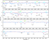 |
Fig. 1 LAMOST spectrum of the PG1159 star RL 104 (blue graph). Overplotted is the final model (red) with Teff = 80 000 K, logg = 6.0, and element abundances as given in Table 4. We note the unusual presence of highly excited C IV lines at locations indicated by horizontal blue and green bars (with principal quantum numbers marked). They are not included in the model. Line identifications in brackets denote lines that are not observed but potentially constrain the atmospheric parameters as discussed in the text. Diffuse interstellar bands (DIBs) are indicated. |
2.2 JL 9 – optical and ultraviolet spectra
To probe the interstellar medium, JL 9 has been observed at UV wavelength with IUE, FUSE, HST, and the ESO VLT (e.g. Diplas & Savage 1994; Hébrard et al. 2005; Lallement et al. 2008; Welty & Crowther 2010; Jenkins 2013). These spectra contain a lot of information on the photosphere of JL 9, which has not been exploited yet. We retrieved an archival spectrum of JL 9 that was recorded on May 19, 2006, with the UVES spectrograph at the ESO Very Large Telescope (ProgID: 077.C-0547(A); PI: R. Lallement). It covers the wavelength regions 3050–3870 and 4785–6809 Å with a resolving power of R ≈ 40 000. Because the UVES observations were tailored to probe the ISM, the wavelength range between ≈4000 and 5000 Å was not covered. However, many important diagnostic lines for the photospheric analysis are located in this range. Therefore, we complemented the UVES spectrum with a spectrum of lower resolution to fill the gap. We employed a spectrum taken on October 6, 1984, with the CASPEC spectrograph attached to the ESO 3.6 m telescope (see Heber et al. 1986; Drilling & Heber 1987). It covers 4042–5085 Å with a spectral resolution of 0.5 Å. It suffered from cosmic ray hits that were not removed.
The spectra are dominated by He II lines, and one very weak neutral helium line (5876 Å) can be detected (Fig. 2). Contributions of weak hydrogen Balmer lines are visible in the respective He II line profiles. Both the Hα and the adjacentHe II line cores are in emission. About thirty metal lines can be identified (Table 2, Fig. 3) and some of them are in emission. They stem from N IV-V and O IV-V. Other metals, in particular carbon, cannot be detected.
We utilised an archival UV spectrum taken with the STIS instrument aboard the Hubble Space Telescope (HST, dataset OBIE16010). It was taken on July 22, 2011, with grating G140M, and it covers the 1191–1245.5 Å wavelength range with a resolution of0.1 Å (Fig. 4). We identified lines from nitrogen, iron, and nickel; namely, N IV, N V, Fe VI, Fe VII, and Ni VI.
In addition, we used two archival far-UV observations taken by the Far Ultraviolet Spectroscopic Explorer (FUSE, data IDs P302120100, U10946010031) with the LWRS aperture that cover the 905–1188 Å range with R ≈ 15 000. These observations consist of five exposures in total with a combined exposure time of about 21 000 s. We retrieved the calibrated and extracted spectra from the Mikulski Archive for Space Telescopes (MAST) for each of the eight detector segment and channel combinations. For each combination, the five exposures were cross-correlated and then co-added. The final spectrum is affected by the ‘worm’, a grid wire shadow on the detector, causing a flux depression longwards of about 1160 Å. We identify broad lines from He II, every other one being blended by interstellar hydrogen Lyman lines (Fig. 5). The majority of lines stems from Ni VI, but we also see lines from iron and from several light metals. They are discussed in detail below.
The far-UV spectrum of JL 9 is affected by strong interstellar lines and was used by Wood et al. (2004) and Jenkins (2013) to study theinterstellar medium (ISM). To account for blends between photospheric and interstellar lines, we constructed a simple model for the ISM. This model uses the interstellar line list distributed with the ISM code OWENS (Lemoine et al. 2002) and considers several IS clouds that are allowed to vary in radial velocity, Doppler broadening, and composition. Our model for JL 9 includes observed lines of H I, D I, C I-II, N I-II, O I, O VI, Si II-III, P II, Ar I, Mn II, Fe I-II, as well as H2 and HD. We refer the reader to Wood et al. (2004) for a quantitative description of the ISM towards JL 9.
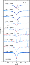 |
Fig. 2 He II lines in CASPEC and UVES spectra of the O(He) star JL 9 (blue). At the bottom, a very weak He I line is depicted. The many spikes in the CASPEC spectra are caused by cosmic ray hits. Overplotted in red is our final model with Teff = 80 000 K, logg = 5.2, and elementabundances as given in Table 4. |
Metal lines identified in the CASPEC and UVES spectra of JL 9.
Components of N V 4946 Å emission line blend in JL 9.
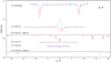 |
Fig. 3 Lines from N IV-V and O IV-V in CASPEC and UVES spectra of the O(He) star JL 9. Overplotted in red is our final model with Teff = 80 000 K, logg = 5.2, and elementabundances as given in Table 4. |
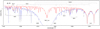 |
Fig. 4 HST/STIS spectrum of the O(He) star JL 9 compared to the final model spectrum (red graph; Teff = 80 000 K, logg = 5.2) with the element abundances given in Table 4. The same model attenuated by interstellar lines is plotted in blue. Prominent photospheric lines are identified. Question marks indicate unidentified lines. A reddening of EB-V = 0.06 was applied to the model spectra. |
2.3 J1418, Gaia DR2 53, and Gaia DR2 67 – Optical spectra
Optical spectra were obtained with the X-shooter instrument at ESO’s Very Large Telescope on May 16, 2016 (ProgID: 297.D-5004(A); PI: S. Geier). They cover the wavelength range 3000–10 000 Å with R ≈ 10 000. With the same instrument setup, Gaia DR2 53 and Gaia DR2 67 were observed on April 10, 2021 (ProgID: 105.206H.001; PI: S. Geier). The spectra of all three He-sdOs are rather similar. They are dominated by He II lines with weak or absent He I lines, indicating a very high temperature at first glance. They all show an Hα line emission core, revealing trace amounts of hydrogen. They also exhibit prominent C IV lines, with the conspicuous exception of Gaia DR2 67 and N V lines.
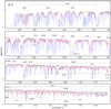 |
Fig. 5 FUSE spectrum of the O(He) star JL 9 compared to the final model spectrum (red graph; Teff = 80 000 K, logg = 5.2) with the element abundances given in Table 4. The same model attenuated by interstellar lines is plotted in blue. |
3 Spectral analysis
3.1 The PG1159 star RL 104
We used the Tübingen Model-Atmosphere Package (TMAP1) to compute non-LTE, plane-parallel, line-blanketed atmosphere models in radiative and hydrostatic equilibrium (Werner & Dreizler 1999; Werner et al. 2003, 2012). We computed models of the type introduced in detail by Werner & Rauch (2014). They were tailored to investigate the optical spectra of relatively cool PG1159 stars. In essence, they consist of the main atmospheric constituents, namely helium, carbon, and oxygen. Nitrogen was included as a trace element in subsequent line-formation iterations, meaning the atmospheric structure was kept fixed.
A problem was encountered because of the presence of C IV lines arising between highly excited levels with principal quantum numbers of n = 7 and 8 for the lower levels and n′ = 13 up to 22 for the upper levels (Fig. 1). Due to linear Stark broadening, they are broad and shallow, and they blend every He II Pickering line (but also the He II Fowler α line at 4686 Å), which are commonly used to constrain the surface gravity. For example, He II 5411 (n = 4–7) is blended by C IV n = 8–14. We cannot model these carbon lines because of the lack of atomic data. However, the effect on the helium line in this case can be estimated by looking at the next highest member of the respective C IV series, namely n = 8–15, which is located in isolation at 5090 Å. As can be expected, the C IV lines with lower level n = 7 are even stronger than those with n = 8, as can be seen, for example, at the isolated n = 7–12 line at 4230 Å. Probably the best gravity indicators are the highest members of the He II Pickering series at 4100 Å and blueward, because the blending C IV lines should be much weaker or virtually absent. With this caveat in mind, we computed a series of model atmospheres by varying Teff, log g and element abundances (He, C, N, O) to gradually approach the final adopted parameter values. Computing a grid of models by systematically varying all parameters was prohibitive, because the model atmospheres turned out to be numerically very unstable in this parameter range. Each single model required extensive care to bring it to convergence.
Our model fitting procedure arrived at Teff = 80 000 ± 5000 K and log g = 6.0 ± 0.5, and abundances He = 0.43, C = 0.38, N = 0.02, O = 0.17 (mass fractions; Table 4). The uncertainty in the abundances is estimated to be 0.3 dex. An upper limit of the hydrogen abundance of H < 3.0 × 10⁻³ was derived. At higher abundances, a Hα emission would be visible in the red wing of the respective He II line. The following considerations constrain the effective temperature and gravity. We can use the temperature dependence of the relative strengths of the lines from N IV/N V and O IV/O V. Looking at models Δ Teff = ± 10 000 K, the lines from ionisation stage IV (e.g. N IV 4708 and 6380 Å, and O IV 4344 and 4389 Å) disappear at too-high temperatures, while the lines from stage V disappear or become too weak at too-low temperatures (e.g. the O V multiplet at 4122 Å). In addition, the unobserved O III multiplet around 3720 Å and the unobserved 3s − 3p doublet of O VI at 3811/3834 Å show up in models that are too cool and too hot, respectively. Also, in too-cool models, C III multiplets at 3885 and 4070 Å are seen, but they are not present in the observed spectrum. Consequently, a good compromise is achieved at Teff = 80 000 K (and logg = 6.0). Increasing and decreasing Teff by 5000 K can roughly be compensated by increasing and decreasing log g by 0.5 dex and 0.3 dex, respectively, such that the IV/V ionisation balances of nitrogen and oxygen hardly change. What do change, however, are the profiles of the He II lines and the C IV lines. Accounting for the uncertainties by blends of the unmodelled, highly excited C IV lines, we think that a good compromise is log g = 6, but we assigned a large conservative error of 0.5 dex.
The N V4945 Å multiplet in the final model is an absorption line that is, however, not observed. In the case of JL 9 presented below, we argue that this line is not a good diagnostic tool because of the uncertainty in atomic data. The strength of the N V 3s − 3p doublet (4604/4620 Å) of the same ion fits quite well. Finally, we take a look at He I 5876 Å. There is a very weak feature in the observation, but it mightnot be real. The line does not appear in our final model, but it would be too strong at lower temperatures or higher gravities, which are outside of our error range.
The radial velocity of RL 104 measured from the LAMOST spectrum amounts to vrad = + 23 ± 10 km s−1 and is listedin Table 4.
Atmospheric properties and derived stellar parameters of the analysed stars.
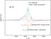 |
Fig. 6 N V 4946 Å emission line in the UVES spectrum of JL 9. It is a blend of three components with uncertain wavelength splittings. Their positions from NIST energy levels and from Hallin (1966) are indicated, where the length of the vertical bars scales with the gf-value. Red graph: Model assuming NIST splitting. Blue graph: Model assuming zero splitting. |
3.2 The O(He) star JL 9
3.2.1 Effective temperature, surface gravity, and H/He ratio
Again, the TMAP code was employed to construct model atmospheres. The models include H, He, C, N, O, Si, P, S, Fe, and Ni. The employed model atoms are described in detail by Werner et al. (2018). In addition, we performed line formation iterations (i.e. keeping the atmospheric structure fixed) for argon using the model atom presented in Werner et al. (2007a).
The atmospheric parameters were inferred from the optical and UV spectra. The employed lines are identified in Figs. 2, 3, 4, and 5. The resulting values are listed in Table 4.
The effective temperature was constrained from elements exhibiting lines from two or three ionisation stages. These are N IV and N V lines in both the optical and UV, O IV and O V lines in the optical plus the O VI resonance doublet in the FUSE spectrum, and Fe VI-VIII lines in the UV. The very weak He I 5876 Å line is also quite temperature sensitive. The ionisation balances of these elements also depend on the surface gravity, which at the same time is constrained by the broad He II lines in the optical and the UV range. An iterative procedure was performed to find the best fit model and to estimate the error ranges. We arrived at Teff = 80 000 ± 5000 K and log g = 5.2 ± 0.3. The hydrogen abundance was determined from the Hα and Hβ lines. It amounts to H =  (mass fraction).
3.2.2 Metal abundances
The carbon abundance was determined from the C IV lines at 1108 and 1169 Å in the FUSE spectrum. For nitrogen, several lines of N IV and N V in the optical as well as in the FUSE and HST spectra were used. O IV and O V lines in the optical and the O VI resonance doublet in the FUSE range served to derive the oxygen abundance.
Other light metal abundances were exclusively constrained from lines in the FUSE spectrum. Fluorine can be studied by the F VI line at 1139.5 Å. However, its identification in JL 9 is uncertain. For silicon, phosphorus, and sulphur we used the lines of Si IV at 1122.5 and 1128.3Å, P V at 1118.0 and 1128.0 Å, and S VI at 933.4, 944.5, 1000.5 and 1117.8 Å. The argon abundance was found from the Ar VII line at 1063.5 Å. The very large number of lines of Fe VI-VIII and Ni VI in the FUSE and HST spectra were used to determine the iron and nickel abundances.
3.2.3 Problems with the N V emission line at 4945 Å
In Fig. 3, we note a significant problem in fitting the N V emission line at 4945 Å. The line is a blend of three transitions between levels with principal quantum numbers n = 6 and 7, namely, 6f–7g, 6g–7h, and 6h–7i. In Fig. 6, we display the situation in detail. The wavelength position of the line blend stems from a laboratory experiment by Hallin (1966), in which this blend was not resolved either. He calculated the positions of these three components (indicated in Fig. 6 and in Table 3). In contrast, if we calculate the components’ positions that follow from level energies listed in the NIST database, they are rather different. The separation is wider, and we employed these positions usually for our spectrum synthesis calculations. Obviously it is too wide because they are inconsistent with the spectrum of JL 9. We observe an asymmetry in the observed line profile such that an emission bump appears in the blue wing, which probably stems from the 6f-7g component whose position seems to be in agreement with the calculation by Hallin (1966). Rieger et al. (1995) reassessed this line blend in laboratory spectra and managed to resolve the 6f–7g component from the others (and assigned a wavelength to it that was consistent with Hallin’s calculation), but still the two other components were not resolved. In order to study what could be the effect of a narrower separation of the line components, we chose the other extreme and shifted all three of them to one and the same wavelength position (4944.46 Å, as measured by Hallin 1966) and carried out the following numerical test. The line overlap was considered in the NLTE iterations for the population numbers and in the final formal solution for the spectrum synthesis in a simplified model atmosphere (less elements, Teff = 80 000, log g = 5.2). The result is shown in Fig. 3. The absorption wings visible in the original model (with NIST splittings) disappear and the central emission at 4944.46 Å is quite pronounced, although the line is not wide enough compared to the observation. A likely explanation is the presence of a weak wind. We conclude that the use of this line as a diagnostic tool is not possible until more precise wavelength measurements are performed in laboratory.
The radial velocity of JL 9 measured from the UVES spectrum is vrad = + 76.4 ± 1.0 km s−1. It agrees with the value of + 77 ± 2 km/s measured by Drilling & Heber (1987) from the very same CASPEC spectrum that we also used for our spectral analysis.
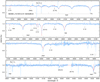 |
Fig. 7 X-shooter spectrum of the He-sdO SDSS J141812.51−024426.8. Emission spikes (except Hα) are cosmic ray hits. Overplotted is the final model (red) with Teff = 70 000 K, logg = 6.0, and elementabundances as given in Table 4. |
3.3 The He-sdOs J1418, Gaia DR2 53, and Gaia DR2 67
The analysis of the optical spectra proceeded in analogy to JL 9. For J1418 we found Teff = 70 000 ± 5000 K and logg = 6.0 ± 0.3. The presence of He I lines helped to constrain the temperature together with the observed lines of C, N, and O (or their absence), while the gravity is indicated by the He II lines. For H, He, C, N, and O, we measured the abundance values given in Table 4. The errors for C on one hand and N and O on the other hand were estimated to ±0.2 and ±0.3 dex, respectively. In the model calculations, the mass fractions for Si, P, S, Fe, and Ni were set to solar. UV spectra would be needed to assess their abundances. The model fit is presented in Fig. 7.
Gaia DR2 53 turned out to be a twin of J1418, except for the effective temperature (see Table 4). For Gaia DR2 53 it is higher by 5000 K because the He I lines at 4471 Å and 5876 Å are weaker. The O abundance can be determined from the very weak O IV triplet at 3730 Å. The model fit is presented in Fig. 8.
Gaia DR2 67 has the same temperature but a slightly higher gravity (75 000 K, log g = 6.3). The main difference to the other He-sdO stars is that carbon cannot be detected. The O IV triplet at 3730 Å is not identified, perhaps because of the lower signal-to-noise ratio of the spectrum. Therefore, only upper limits for C and O were derived.
We measured the radial velocities of the three He-sdOs and list them in Table 4. The value for J1418 (vrad = −55 ± 3 km s−1) is in agreement with the one we measured from the SDSS spectrum (− 55 ± 10 km s−1) that was analysed by Werner et al. (2014)2.
4 Physical parameters
4.1 SED fitting, stellar radii, luminosities, and distances
With well-known distances, d, from the Gaia EDR3 (Gaia Collaboration 2021), it is now possible to determine the radius, R, luminosity, L, and mass, M, of a star, if its effective temperature and surface gravity are known from spectroscopy. For that, one needs to perform a fit to the observed SED which takes into account the effect of interstellar reddening. The observed flux, fλ, relates to the (reddened) model flux, Fλ, via fλ = FλπR2∕d2. In order to derive the radii of our stars, we used the distances reported by Bailer-Jones et al. (2021) and then (using the Fitzpatrick (1999) reddening law) varied the values for EB-V and the radius, until a good agreement of our best fitting model fluxes from our spectral analysis to the observed SED was found. We employed photometry from various catalogues: GALEX (Bianchi et al. 2017), Pan-STARRS1 (Flewelling et al. 2020), Landolt B, V (Henden et al. 2015), Gaia (Gaia Collaboration 2021), SkyMapper (Wolf et al. 2018), SDSS (Alam et al. 2015), 2MASS (Cutri et al. 2003), and WISE (Schlafly et al. 2019). Magnitudes were converted into fluxes using the VizieR Photometry viewer3. In the case of JL 9,the FUSE and IUE spectra were also employed for the fit. The resulting values for the reddening and radii are listed in Table 4. This table also lists the luminosities of our stars that were calculated from the radii and effective temperatures via  . In Fig. 10, our SED fits are shown. It can be seen that the SEDs of all our five stars are reproduced nicely and there is no sign of a companion or a disk.
To evaluate the spectroscopic distances of the stars, we must consider the effect of interstellar reddening. The visual extinction is evaluated from the standard relation AV = 3.1×EB-V, so we obtain a dereddened visual magnitude V0. The spectroscopic distance d is found by the relation
![\[ d \textrm{[pc]}= 7.11\times 10^{4} \sqrt{H_{\nu}\cdot M\cdot 10^{0.4 V_0-\log g}} \]](/articles/aa/full_html/2022/02/aa42397-21/aa42397-21-eq4.png)
where Hν is the Eddington flux of the best-fit atmosphere model at 5400 Å (Table 4). The results are listed in Table 4 as well as the distances derived from the Gaia EDR3 parallaxes (Bailer-Jones et al. 2021). The main error source for the spectroscopic distance is the uncertainty in the surface gravity. Both distance determinations agree within error limits except for Gaia DR2 67 for which the parallax distance is a factor of two larger. We note that similar problems were encountered and discussed, for instance, in spectroscopic analyses of hot WDs (Preval et al. 2019) and hot post-AGB stars (Herrero et al. 2020).
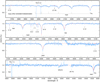 |
Fig. 8 X-shooter spectrum of the He-sdO Gaia DR2 53. Emission spikes (except Hα) are cosmic ray hits. Overplotted is the final model (red) with Teff = 75 000 K, logg = 6.0, and elementabundances as given in Table 4. |
4.2 Stellar masses
Figures 11 and 12 show the position of the analysed stars in the Teff –logg diagram. Their masses are determined by comparison with evolutionary tracks by linear interpolation or extrapolation. The errors are dominated by the uncertainty in g. From Fig. 11, we find the mass of the PG1159 star RL 104 by comparison with tracks for stars that experienced a very late thermal pulse (VLTP; Miller Bertolami & Althaus 2006). It is  . For the O(He) star JL 9, these tracks imply
  . Alternatively, the stellar merger tracks in Fig. 12 yield
  . For the He-sdOs, the masses are derived from the merger tracks and listed in Table 4.
Because the distances are well known by the Gaia parallax measurements, the stellar masses can be determined in an alternative way. From the SED fit that used the Gaia distance, we know the stellar radius R. Together with the spectroscopically determined surface gravity g, we obtain the mass from  . However, the large uncertainty in g (factors 3.2 and 2 for RL 104 and the other for stars, respectively) directly propagate into the mass determination. For RL 104, JL 9, J1418, Gaia DR2 53, and Gaia DR2 67, we find M∕M⊙ =
  ,
,  ,
,  ,
,  , and
, and  , respectively.The values are formally consistent with the masses found from the evolutionary tracks, but cannot further constrain them.
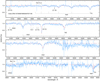 |
Fig. 9 X-shooter spectrum of the He-sdO Gaia DR2 67. Emission spikes (except Hα) are cosmic ray hits. Overplotted is the final model (red) with Teff = 75 000 K, logg = 6.3, and elementabundances as given in Table 4. |
5 Discussion and summary
Our three analysed He-sdOs are located below the helium main sequence and we identify them with evolved, He-shell burning post-EHB stars that either formed from a binary WD merger or by single star evolution with a late helium core flash. The O(He) star JL 9 is a more luminous object that lies in the post-AGB region of the Kiel diagram. The abundance pattern of O(He) stars cannot be explained by (V)LTP models (Reindl et al. 2014b), and hence we discuss its evolution in the context of a binary He-WD merger. The PG1159 star RL 104 is discussed as a (V)LTP object, as is usual for this stars in this spectral class (Werner & Herwig 2006). However, in light of its low mass, a binary WD merger model is also considered. The different evolutionary scenarios are discussed with regard to determined abundance patterns that are displayed in Fig. 13.
5.1 Evolution of the O(He) star JL 9 and the three He-sdOs
The He/H number abundance ratio in our three He-sdOs is log y = 0.35. This is, for example, in good agreement with the values found for many hot He-sdOs, including those in the GALEX sample (Németh et al. 2012), which is around logy = 0.6 (Heber 2016).
As for the C and N abundances, the abundance patterns of our He-sdOs are similar to other stars of this class. In Gaia DR2 67, we see a clear hint to CNO burning. N is strongly enriched compared to the Sun, while C and O are depleted. In J1418 and Gaia DR2 53, C is enriched by He-burning while O is depleted. Heber & Hirsch (2010) showed that in their ESO/SPY sample all objects with Teff > 43 000 K are carbon dominated (C/N > 1, by mass; see also Stroeer et al. 2007 and Schindewolf et al. 2018). In stark contrast to these 15 objects, Gaia DR2 67 is nitrogen dominated (N/C > 3.5). Oxygen abundance measurements in He-sdOs are rather scarce. For four objects with Teff around 45 000 K, Schindewolf et al. (2018) found logarithmic mass fractions between − 4.2 and − 2.9. For J1418 and Gaia DR2 53 we determined an intermediate value of − 3.2 and an upper limit of − 2.7 for Gaia DR2 67. For the O(He) star we found a strong N enrichment (− 2.2) whereas C and O are strongly depleted (− 4.2 and − 4.1, respectively).
We compare the abundances of our He-sdOs and the O(He) star to surface abundance predictions by the binary He-WD merger models of Zhang & Jeffery (2012a). They comprise different merger scenarios, a slow (cool) merger, a fast (hot) merger, and a combination of both (composite merger). In the first case, the merger product exhibits the compositionof the accreted WD, that is He-rich matter as CNO burning ash with C and O transformed into N. In the second case, nuclear burning and mixing changes the abundances in favor of He-burning ashes, creating C overabundances and depleting N. The composite merger combines both processes. In this case, mergers with M < 0.7 M⊙ are N rich, while more massive ones are C rich with significant N abundance.
For the He-sdO Gaia DR2 67 and the O(He) star JL 9, we have N oversolar and C and O depleted; hence, this fits the cold-merger model. CNO abundances of three of the four O(He) stars analysed by Reindl et al. (2014a) show a similar behaviour. The high C/N = 10 mass ratio in J1418 and Gaia DR2 53, however, requires composite-merger models (because of the presence of N, a fast-merger model does not fit) with high merger mass (0.8 M⊙), because they have efficient dredge up of C-rich material from the stellar core. However, this is at odds with the spectroscopic masses  and
and  . Another disaccord is the relatively high hydrogen abundance that we found in the O(He) star and the He-sdOs (6 and 10% by mass). The merger models predict much lower abundances (Hall & Jeffery 2016; Schwab 2018; Jeffery & Zhang 2020). The abundances of heavier elements in JL 9 (Si, P, S, Ar, Fe, and Ni) are essentially solar, reflecting the original composition of the star.
The late hot flasher scenario is the alternative explanation for the origin of He-sdOs. Usually, a helium-core flash occurs at the tip of the red giant branch (RGB). However, this flash can also occur when a star leaves the RGB to become a WD or even when it is a WD. In the latter case, the star is termed a late hot flasher, and the flash-driven convection reaches the surface layer altering the chemical composition. The scenario has two types, namely a shallow mixing (SM) case and deep mixing (DM) case. In the first case, hydrogen is ingested into the stellar interior and diluted such that the surface abundance of H is reduced, while in the second case H is ingested an burned and only minute quantities of H remain visible on the surface. We compared the surface abundances predicted by models for late hot flashers from Battich et al. (2018) with those of our three analysed He-sdOs. For that, we chose the model with metallicity Z = 0.02 and initial helium abundance He = 0.285. One immediately faces the problem that, in the SM case, the predicted hydrogen abundance (H = 0.47) is much higher than the observations (H = 0.10), and in the DM case the prediction is much lower (0.0036 or even smaller, depending on details in the modelling). The SM model also predicts C four times lower and N ten times higher than observed for J1418 and Gaia DR2 53. For Gaia DR2 53, the predicted nitrogen abundance (N = 0.0062) agrees with the observed one (N = 0.0035) within error limits (0.5 dex), just like the predicted C and N abundances (C = 0.0015, O = 0.0062) with the upper limits from the observations (C < 0.001, O < 0.002). For the O(He) star JL 9, the observed C and O abundances are by more than 1 dex below the hot-flasher prediction and, like forthe He-sdOs, the observed hydrogen abundance (H = 0.058) cannot be fitted by the DM and SM models.
In essence, the main obstacle for both, the merger model and the hot flasher model is the failure to explain the observed hydrogen abundance in our He-sdOs. The O(He) star’s CNO abundances are in accordance with the merger model, but not its high hydrogen content.
In this context, we note that Zhang et al. (2017) pointed out that hot subdwarfs with intermediate H and He abundances (He number fractions 10–90%) can be formed by mergers of a main-sequence star with a helium WD. However, their models predict that the atmospheres of the merger remnants become pure hydrogen even before they reach the helium main sequence because of the gravitational settling of helium and metals.
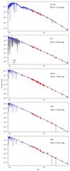 |
Fig. 10 Comparison of our best fitting model fluxes (blue) with the observed photometry (red; in the case of JL 9, the FUSE and IUE spectra are shown in grey). The reddening that has been applied to the model fluxes is indicated in each panel. |
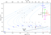 |
Fig. 11 Position of our programme stars in the Teff–logg diagram, in comparison with other PG1159 stars (black squares) and DO white dwarfs (red circles). Blue lines are VLTP post-AGB evolutionary tracks (labelled with stellar mass in M⊙) from Miller Bertolami & Althaus (2006). Indicated is the PG1159 wind limit according to Unglaub & Bues (2000). No PG 1159 stars are found below it because radiation-driven stellar winds become so weak that they can no longer prevent gravitational settling of heavy elements. |
5.2 Evolution of the PG1159 star RL 104
The atmospheric composition of RL 104 (He = 0.43, C = 0.38, N = 0.02, O = 0.17, mass fractions) is typical for PG1159 stars. The prototype PG1159−035, for instance, has He = 0.35, C = 0.48, N = 0.001, and O = 0.17 (Werner & Herwig 2006). Using the VLTP tracks, we derived a mass of  for RL 104. It is one of the lowest masses found for any PG1159 star, beaten only by HS 0704 + 6153, which has a comparably low mass of M = 0.47M⊙ (Dreizler & Heber 1998; Miller Bertolami & Althaus 2006). The difference between the two objects is, however, that RL 104 is a He-shell burner evolving towards higher effective temperatures, while HS 0704 + 6153 is already on the WD cooling track (logg = 7.5), it being the coolest PG1159 star to date (Teff = 75 000 K). Therefore, RL 104 is the coolest PG1159 star (Teff = 80 000 K) hitherto found in a pre-WD evolutionary stage (logg = 6.0). The presence of nitrogen is an indicator that the star suffered a very late thermal pulse and not another variant, namely a late thermal pulse or an AGB final thermal pulse (AFTP). For a detailed discussion of these scenarios we invite the reader to consult, for example, Werner & Herwig (2006).
From the fact that RL 104 is located among the hottest He-sdOs in the log g–Teff diagram, it is tempting to consider that it is the outcome of a binary WD merger. However, the binary merger models of two He-WDs of Zhang & Jeffery (2012a) predict helium-dominated envelopes and cannot explain the high-C and -O content in the atmosphere of RL 104. The situation is different when both merging WDs have a C/O core. Recently, Schwab & Bauer (2021) presented calculations in order to predict the outcome of a close binary system consisting of a hot subdwarf and a WD, which is a new class of Roche-lobe filling binaries where the subdwarfs transfer mass to the WD companion (Kupfer et al. 2020a,b). The subdwarf will evolve into a low-mass C/O core WD with a thick helium layer, and it will finally merge with the more massive C/O WD. Schwab & Bauer (2021) followed the post-merger evolution after constructing an initial model in which a 0.55 M⊙ C/O WD accreted matter from the 0.36 M⊙ C/O remnant of a He-sdO. In the pre-WD phase (steady He-shell burning) of the merger, the surface abundances are about He = 0.30, C = 0.26, N = 0.004, and O = 0.44. Considering the error limits of our abundance determination in RL 104 (0.3 dex), the abundance pattern from this model is similar to the observation. The very low hydrogen abundance H = 0.001 in the merger model is in accordance with our detection threshold of H <0.003. The high mass of the merger model (≈ 0.9 M⊙) is, however, at odds with that of RL 104 derived from the merger models of Zhang & Jeffery (2012a) in Fig. 12 ( ).
).
Just before reaching the WD sequence, the high-mass He-WD+He-WD merger model sequences (0.7 and 0.8 M⊙) of Zhang & Jeffery (2012a) display a small loop caused by a final He-shell flash (Fig. 12). One can speculate that it initiates envelope convection, creating PG1159-like abundances similar to the VLTP scenario in single star evolution. Maybe with enhanced physical models, such a late He-shell flash could also occur in lower mass mergers (Josiah Schwab, priv. comm.), explaining the existence of low-mass PG1159 stars such as RL 104.
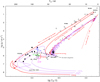 |
Fig. 12 Position of our programme stars in the Teff–logg diagram among other O(He) stars (full circles) as well as RCB stars (crosses), EHe stars (open circles), and He-sdOs (squares), see Reindl et al. (2014b) and references therein. Red and purple lines are evolutionary tracks for a composite-merger scenario of two He-WDs (marked with the merger mass in M⊙) from Zhang & Jeffery (2012b). The dashed black line is the zero-age helium main sequence. |
 |
Fig. 13 Abundances measured in our programme stars. Arrows indicate upper limits. The black line represents solar values. |
Acknowledgements
We thank Uli Heber for putting his CASPEC spectrum of JL 9 at our disposal and useful comments on an earlier version of the manuscript, and Max Pritzkuleit for his support of the HOTFUSS project. M.D. acknowledges funding by the Deutsche Forschungsgemeinschaft (DFG) through grant HE1356/71-1. R.R. has receivedfunding from the postdoctoral fellowship programme Beatriu de Pinós, funded by the Secretary of Universities and Research (Government of Catalonia) and by the Horizon 2020 programme of research and innovation of the European Union under the Maria Skłodowska-Curie grant agreement No 801370. The TMAD tool (http://astro.uni-tuebingen.de/~TMAD) used for this paper was constructed as part of the activities of the German Astrophysical Virtual Observatory. Some of the data presented in this paper were obtained from the Mikulski Archive for Space Telescopes (MAST). This research has made use of NASA’s Astrophysics Data System and the SIMBAD database, operated at CDS, Strasbourg, France. This research has made use of the VizieR catalogue access tool, CDS, Strasbourg, France. This work has made use of data from the European Space Agency (ESA) mission Gaia.
References
- Alam, S., Albareti, F. D., Allende Prieto, C., et al. 2015, ApJS, 219, 12 [Google Scholar]
- Asplund, M., Grevesse, N., Sauval, A. J., & Scott, P. 2009, ARA&A, 47, 481 [NASA ADS] [CrossRef] [Google Scholar]
- Bailer-Jones, C. A. L., Rybizki, J., Fouesneau, M., Demleitner, M., & Andrae, R. 2021, AJ, 161, 147 [Google Scholar]
- Battich, T., Miller Bertolami, M. M., Córsico, A. H., & Althaus, L. G. 2018, A&A, 614, A136 [NASA ADS] [CrossRef] [EDP Sciences] [Google Scholar]
- Bianchi, L., Shiao, B., & Thilker, D. 2017, ApJS, 230, 24 [Google Scholar]
- Chromey, F. R. 1979, AJ, 84, 534 [NASA ADS] [CrossRef] [Google Scholar]
- Cutri, R. M., Skrutskie, M. F., van Dyk, S., et al. 2003, VizieR Online Data Catalog: II/246 [Google Scholar]
- De Marco, O., Long, J., Jacoby, G. H., et al. 2015, MNRAS, 448, 3587 [Google Scholar]
- Diplas, A., & Savage, B. D. 1994, ApJS, 93, 211 [NASA ADS] [CrossRef] [Google Scholar]
- Dreizler, S., & Heber, U. 1998, A&A, 334, 618 [NASA ADS] [Google Scholar]
- Drilling, J. S., & Heber, U. 1987, in IAU Colloq. 95: Second Conference on Faint Blue Stars, eds. A. G. D. Philip, D. S. Hayes, & J. W. Liebert, 603 [Google Scholar]
- Fitzpatrick, E. L. 1999, PASP, 111, 63 [Google Scholar]
- Flewelling, H. A., Magnier, E. A., Chambers, K. C., et al. 2020, ApJS, 251, 7 [NASA ADS] [CrossRef] [Google Scholar]
- Frew, D. J., Bojičić, I. S., Parker, Q. A., et al. 2014, MNRAS, 440, 1345 [NASA ADS] [CrossRef] [Google Scholar]
- Gaia Collaboration 2018, VizieR Online Data Catalog: I/345 [Google Scholar]
- Gaia Collaboration (Brown, A. G. A., et al.) 2021, A&A, 649, A1 [NASA ADS] [CrossRef] [EDP Sciences] [Google Scholar]
- Geier, S. 2020, A&A, 635, A193 [NASA ADS] [CrossRef] [EDP Sciences] [Google Scholar]
- Geier, S., Raddi, R., Gentile Fusillo, N. P., & Marsh, T. R. 2019, A&A, 621, A38 [NASA ADS] [CrossRef] [EDP Sciences] [Google Scholar]
- Hall, P. D., & Jeffery, C. S. 2016, MNRAS, 463, 2756 [NASA ADS] [CrossRef] [Google Scholar]
- Hallin, R. 1966, Arkiv för Fysik, 31, 511 [Google Scholar]
- Heber, U. 2016, PASP, 128, 082001 [Google Scholar]
- Heber, U., & Hirsch, H. 2010, in AIP Conf. Ser., 1314, International Conference on Binaries: in celebration of Ron Webbink’s 65th Birthday, eds. V. Kalogera, & M. van der Sluys, 79 [Google Scholar]
- Heber, U., Drilling, J. S., & Husfeld, D. 1986, in IAU Colloq. 87: Hydrogen Deficient Stars and Related Objects, eds. K. Hunger, D. Schoenberner, & N. Kameswara Rao, 345 [CrossRef] [Google Scholar]
- Hébrard, G., Tripp, T. M., Chayer, P., et al. 2005, ApJ, 635, 1136 [CrossRef] [Google Scholar]
- Henden, A. A., Levine, S., Terrell, D., & Welch, D. L. 2015, in American Astronomical Society Meeting Abstracts, 225, 336.16 [NASA ADS] [Google Scholar]
- Herrero, A., Parthasarathy, M., Simón-Díaz, S., et al. 2020, MNRAS, 494, 2117 [NASA ADS] [CrossRef] [Google Scholar]
- Hobbs, L. M., York, D. G., Snow, T. P., et al. 2008, ApJ, 680, 1256 [NASA ADS] [CrossRef] [Google Scholar]
- Jaidee, S., & Lyngå, G. 1969, Arkiv Astronomi, 5, 345 [NASA ADS] [Google Scholar]
- Jeffery, C. S., & Zhang, X. 2020, JApA, 41, 48 [NASA ADS] [Google Scholar]
- Jenkins, E. B. 2013, ApJ, 764, 25 [NASA ADS] [CrossRef] [Google Scholar]
- Kupfer, T., Bauer, E. B., Burdge, K. B., et al. 2020a, ApJ, 898, L25 [Google Scholar]
- Kupfer, T., Bauer, E. B., Marsh, T. R., et al. 2020b, ApJ, 891, 45 [Google Scholar]
- Lallement, R., Hébrard, G., & Welsh, B. Y. 2008, A&A, 481, 381 [NASA ADS] [CrossRef] [EDP Sciences] [Google Scholar]
- Lei, Z., Zhao, J., Németh, P., & Zhao, G. 2020, ApJ, 889, 117 [NASA ADS] [CrossRef] [Google Scholar]
- Lemoine, M., Vidal-Madjar, A., Hébrard, G., et al. 2002, ApJS, 140, 67 [NASA ADS] [CrossRef] [Google Scholar]
- Miller Bertolami, M. M., & Althaus, L. G. 2006, A&A, 454, 845 [NASA ADS] [CrossRef] [EDP Sciences] [Google Scholar]
- Németh, P., Kawka, A., & Vennes, S. 2012, MNRAS, 427, 2180 [Google Scholar]
- Preval, S. P., Barstow, M. A., Bainbridge, M., et al. 2019, MNRAS, 487, 3470 [NASA ADS] [CrossRef] [Google Scholar]
- Reindl, N., Rauch, T., Werner, K., et al. 2014a, A&A, 572, A117 [NASA ADS] [CrossRef] [EDP Sciences] [Google Scholar]
- Reindl, N., Rauch, T., Werner, K., Kruk, J. W., & Todt, H. 2014b, A&A, 566, A116 [NASA ADS] [CrossRef] [EDP Sciences] [Google Scholar]
- Reindl, N., Geier, S., Kupfer, T., et al. 2016, A&A, 587, A101 [NASA ADS] [CrossRef] [EDP Sciences] [Google Scholar]
- Rieger, G., Boduch, P., Chantepie, M., et al. 1995, Phys. Scr, 52, 166 [NASA ADS] [CrossRef] [Google Scholar]
- Rubin, V. C., Westpfahl, D., J., & Tuve, M. 1974, AJ, 79, 1406 [NASA ADS] [CrossRef] [Google Scholar]
- Saio, H., & Jeffery, C. S. 2002, MNRAS, 333, 121 [CrossRef] [Google Scholar]
- Schindewolf, M., Németh, P., Heber, U., et al. 2018, A&A, 620, A36 [NASA ADS] [CrossRef] [EDP Sciences] [Google Scholar]
- Schlafly, E. F., Meisner, A. M., & Green, G. M. 2019, ApJS, 240, 30 [Google Scholar]
- Schwab, J. 2018, MNRAS, 476, 5303 [Google Scholar]
- Schwab, J., & Bauer, E. B. 2021, ApJ, 920, 110 [NASA ADS] [CrossRef] [Google Scholar]
- Stassun, K. G., Oelkers, R. J., Paegert, M., et al. 2019, AJ, 158, 138 [Google Scholar]
- Stroeer, A., Heber, U., Lisker, T., et al. 2007, A&A, 462, 269 [NASA ADS] [CrossRef] [EDP Sciences] [Google Scholar]
- Unglaub, K., & Bues, I. 2000, A&A, 359, 1042 [NASA ADS] [Google Scholar]
- Welty, D. E., & Crowther, P. A. 2010, MNRAS, 404, 1321 [NASA ADS] [Google Scholar]
- Werner, K., & Dreizler, S. 1999, J. Comput. Appl. Math., 109, 65 [NASA ADS] [CrossRef] [Google Scholar]
- Werner, K., & Herwig, F. 2006, PASP, 118, 183 [Google Scholar]
- Werner, K., & Rauch, T. 2014, A&A, 569, A99 [NASA ADS] [CrossRef] [EDP Sciences] [Google Scholar]
- Werner, K., & Rauch, T. 2015, A&A, 583, A131 [NASA ADS] [CrossRef] [EDP Sciences] [Google Scholar]
- Werner, K., Deetjen, J. L., Dreizler, S., et al. 2003, in ASP Conf. Ser., 288, Stellar Atmosphere Modeling, eds. I. Hubeny, D. Mihalas, & K. Werner, 31 [Google Scholar]
- Werner, K., Rauch, T., & Kruk, J. W. 2007a, A&A, 466, 317 [NASA ADS] [CrossRef] [EDP Sciences] [Google Scholar]
- Werner, K., Rauch, T., & Kruk, J. W. 2007b, A&A, 474, 591 [NASA ADS] [CrossRef] [EDP Sciences] [Google Scholar]
- Werner, K., Dreizler, S., & Rauch, T. 2012, Astrophysics Source Code Library [record ascl:1212.015] [Google Scholar]
- Werner, K., Rauch, T., & Kepler, S. O. 2014, A&A, 564, A53 [NASA ADS] [CrossRef] [EDP Sciences] [Google Scholar]
- Werner, K., Rauch, T., & Kruk, J. W. 2018, A&A, 609, A107 [NASA ADS] [CrossRef] [EDP Sciences] [Google Scholar]
- Wolf, C., Onken, C. A., Luvaul, L. C., et al. 2018, PASA, 35, e010 [Google Scholar]
- Wood, B. E., Linsky, J. L., Hébrard, G., et al. 2004, ApJ, 609, 838 [NASA ADS] [CrossRef] [Google Scholar]
- Zhang, X., & Jeffery, C. S. 2012a, MNRAS, 426, L81 [NASA ADS] [CrossRef] [Google Scholar]
- Zhang, X., & Jeffery, C. S. 2012b, MNRAS, 419, 452 [NASA ADS] [CrossRef] [Google Scholar]
- Zhang, X., Hall, P. D., Jeffery, C. S., & Bi, S. 2017, ApJ, 835, 242 [NASA ADS] [CrossRef] [Google Scholar]
We note that the SDSS spectra analysed by Werner et al. (2014) were shifted from vacuum to rest wavelengths by amounts given in their Table 3.
All Tables
All Figures
|
Fig. 1 LAMOST spectrum of the PG1159 star RL 104 (blue graph). Overplotted is the final model (red) with Teff = 80 000 K, logg = 6.0, and element abundances as given in Table 4. We note the unusual presence of highly excited C IV lines at locations indicated by horizontal blue and green bars (with principal quantum numbers marked). They are not included in the model. Line identifications in brackets denote lines that are not observed but potentially constrain the atmospheric parameters as discussed in the text. Diffuse interstellar bands (DIBs) are indicated. |
| In the text | |
|
Fig. 2 He II lines in CASPEC and UVES spectra of the O(He) star JL 9 (blue). At the bottom, a very weak He I line is depicted. The many spikes in the CASPEC spectra are caused by cosmic ray hits. Overplotted in red is our final model with Teff = 80 000 K, logg = 5.2, and elementabundances as given in Table 4. |
| In the text | |
|
Fig. 3 Lines from N IV-V and O IV-V in CASPEC and UVES spectra of the O(He) star JL 9. Overplotted in red is our final model with Teff = 80 000 K, logg = 5.2, and elementabundances as given in Table 4. |
| In the text | |
|
Fig. 4 HST/STIS spectrum of the O(He) star JL 9 compared to the final model spectrum (red graph; Teff = 80 000 K, logg = 5.2) with the element abundances given in Table 4. The same model attenuated by interstellar lines is plotted in blue. Prominent photospheric lines are identified. Question marks indicate unidentified lines. A reddening of EB-V = 0.06 was applied to the model spectra. |
| In the text | |
|
Fig. 5 FUSE spectrum of the O(He) star JL 9 compared to the final model spectrum (red graph; Teff = 80 000 K, logg = 5.2) with the element abundances given in Table 4. The same model attenuated by interstellar lines is plotted in blue. |
| In the text | |
|
Fig. 6 N V 4946 Å emission line in the UVES spectrum of JL 9. It is a blend of three components with uncertain wavelength splittings. Their positions from NIST energy levels and from Hallin (1966) are indicated, where the length of the vertical bars scales with the gf-value. Red graph: Model assuming NIST splitting. Blue graph: Model assuming zero splitting. |
| In the text | |
|
Fig. 7 X-shooter spectrum of the He-sdO SDSS J141812.51−024426.8. Emission spikes (except Hα) are cosmic ray hits. Overplotted is the final model (red) with Teff = 70 000 K, logg = 6.0, and elementabundances as given in Table 4. |
| In the text | |
|
Fig. 8 X-shooter spectrum of the He-sdO Gaia DR2 53. Emission spikes (except Hα) are cosmic ray hits. Overplotted is the final model (red) with Teff = 75 000 K, logg = 6.0, and elementabundances as given in Table 4. |
| In the text | |
|
Fig. 9 X-shooter spectrum of the He-sdO Gaia DR2 67. Emission spikes (except Hα) are cosmic ray hits. Overplotted is the final model (red) with Teff = 75 000 K, logg = 6.3, and elementabundances as given in Table 4. |
| In the text | |
|
Fig. 10 Comparison of our best fitting model fluxes (blue) with the observed photometry (red; in the case of JL 9, the FUSE and IUE spectra are shown in grey). The reddening that has been applied to the model fluxes is indicated in each panel. |
| In the text | |
|
Fig. 11 Position of our programme stars in the Teff–logg diagram, in comparison with other PG1159 stars (black squares) and DO white dwarfs (red circles). Blue lines are VLTP post-AGB evolutionary tracks (labelled with stellar mass in M⊙) from Miller Bertolami & Althaus (2006). Indicated is the PG1159 wind limit according to Unglaub & Bues (2000). No PG 1159 stars are found below it because radiation-driven stellar winds become so weak that they can no longer prevent gravitational settling of heavy elements. |
| In the text | |
|
Fig. 12 Position of our programme stars in the Teff–logg diagram among other O(He) stars (full circles) as well as RCB stars (crosses), EHe stars (open circles), and He-sdOs (squares), see Reindl et al. (2014b) and references therein. Red and purple lines are evolutionary tracks for a composite-merger scenario of two He-WDs (marked with the merger mass in M⊙) from Zhang & Jeffery (2012b). The dashed black line is the zero-age helium main sequence. |
| In the text | |
|
Fig. 13 Abundances measured in our programme stars. Arrows indicate upper limits. The black line represents solar values. |
| In the text | |
Current usage metrics show cumulative count of Article Views (full-text article views including HTML views, PDF and ePub downloads, according to the available data) and Abstracts Views on Vision4Press platform.
Data correspond to usage on the plateform after 2015. The current usage metrics is available 48-96 hours after online publication and is updated daily on week days.
Initial download of the metrics may take a while.