© ESO 2021

1. Introduction

The solar wind is a plasma of a very controversial nature due to the multitude of physical processes which act concomitantly or successively and control not only local properties, but also the variation of plasma parameters with the expansion in heliosphere. Indeed, the solar wind is neither a collision-dominated plasma nor a collisionless one (Maksimovic et al. 1997; Pierrard et al. 2011), and this is most likely the reason why ideal magnetohydrodynamic (MHD) or collision-free (exospheric) models cannot accurately reproduce the global expansion and thermodynamics of the solar wind (Maksimovic et al. 1997; Matteini et al. 2007; Bale et al. 2013). Particle-particle collisions are believed to play an important role at low distances from the Sun in the outer corona, although there are also wave fluctuations and turbulence from MHD to proton and electron scales (Bourouaine et al. 2012). At larger heliocentric distances, for example at 1 AU, low-energy particle (core) populations remain organized by a so-called collisional age (Salem et al. 2003; Štverák et al. 2008; Bale et al. 2009), while the nonequilibrium states of plasma particles with anisotropic velocity (or energy) distributions and suprathermal populations (Maksimovic et al. 2005; Marsch 2006; Wilson et al. 2019) may be explained by the interaction with wave turbulence and small-scale fluctuations (Štverák et al. 2008; Bale et al. 2009; Alexandrova et al. 2013). There is observational evidence for the preferential heating of plasma particles through resonant wave-particle interactions (Bourouaine et al. 2011; Wilson et al. 2013), as well as for the generation of more diffuse suprathermal (halo) populations by the wave turbulence of a quiet solar wind, or by the instabilities self-induced by the beam (or strahl) populations in the fast solar winds, interplanetary shocks, etc. (Mason & Gloeckler 2012; Gurgiolo et al. 2016).

Suprathermal populations enhance the high energy tails of the observed velocity distributions (up to a few keV) and are characteristic not only of the solar wind electrons and protons (see Lazar et al. 2012 for a review), but they are also reported for the heavier (minor) ions at 1 AU (Collier et al. 1996) and beyond (Ogilvie et al. 1993). Theoretical approaches use the so-called Kappa distributions to describe these populations (Pierrard & Lazar 2010) and offer explanations for their origin, mainly based on the energization of plasma particles, for example, electrons, by the interaction with small-scale wave fluctuations, including for instance the electromagnetic electron-cyclotron (whistler) waves (Vocks et al. 2008) or the electrostatic Langmuir plasma waves (Viñas et al. 2000; Yoon et al. 2006). Quasi-linear models involve collisions and a weak plasma turbulence, either with predefined spectral profiles (Roberts & Miller 1998; Vocks et al. 2008), or self-supported by spontaneous and induced plasma wave fluctuations (Yoon et al. 2006). What matters is that suprathermal populations retain the effects of wave turbulence and fluctuations present in the system, suggesting that a realistic macroscopic theory for the energy and particle transport in space plasmas must rely on the assumption that plasma particles are Kappa-distributed.

Transport processes in a plasma can be studied with a transport equation, such as the (collisional) Boltzmann equation for the evolution of the phase space particle distribution. If a plasma is sufficiently homogeneous, macroscopic equations are obtained by calculating the main velocity moments on the basis of a velocity distribution function describing the plasma particles (Braginskii 1965; Balescu 1988). The macroscopic equations are based on a linear relationship between the fluxes and the external forces and gradients (in, e.g., density, temperature, pressure) driving the fluxes. The constants of proportionality are called transport coefficients, and they contain valuable physical information. The collisional term in the transport equation describes the rate of change of the distribution due to collisions, and by adopting simplified models for the collision term (see Sect. 3), one can obtain analytical expressions for the transport coefficients. Because driving gradients and forces lead to deviations from quasi-stationary states, one can assume a small or linear perturbation of the distribution function and linearize the transport equation (Goedbloed et al. 2019). For plasmas near thermal equilibrium, the standard Maxwellian distribution is commonly used, while nonthermal particle populations in space plasmas are well described by the family of Kappa distributions (see Sect. 2).

Recent studies of plasma diffusion, that is, the flux of particles due to a density gradient in the plasma, concerned nonequilibrium plasmas and applied Kappa distributions to determine the diffusion coefficient (Wang & Du 2017; Ebne Abbasi et al. 2017). In addition to the diffusion, the mobility coefficient describes the flux of charged particles in the presence of an electrical field and was examined involving Maxwellian (Hagelaar & Pitchford 2005) and Kappa distributions (Wang & Du 2017). The mobility of charged particles is related to the electric conductivity, setting the current density, and the electric field in the relationship (Du 2013; Ebne Abbasi et al. 2017). The thermoelectric coefficient relates the electric field to the temperature gradient resulting in electric voltages and currents, and it was derived based on Kappa distributions (Du 2013; Guo & Du 2019). The heat flux is driven by a temperature gradient, for which the thermal conductivity is the constant of proportionality, see, for example, Rat et al. (2001) for Maxwellian plasma populations, and Du (2013), Guo & Du (2019), and Ebne Abbasi & Esfandyari-Kalejahi (2019) using Kappa distributions. However, all of these studies involving Kappa distributions invoke a modified approach that drastically differs from the original Olbertian or the standard Kappa distribution introduced by Olbert (1968) and Vasyliūnas (1968). Moreover, recent studies have also pointed to the differences between these two Kappa approaches (Lazar et al. 2015, 2016), clearly stating that a modified Kappa distribution does not allow for a proper comparison with the quasi-thermal core of the observed distributions to outline the suprathermals and their implications (see also Sect. 2 for more details as well as the discussions in Lazar & Fichtner 2021).

Motivated by these precedents, in this paper we propose a re-evaluation of transport coefficients based on a standard Kappa approach, which allows for a correct assessment of the contribution of the suprathermal population. Indeed, here we show that a modified approach systematically leads to an underestimation of the effects of these populations on transport coefficients. The paper is structured as follows. In Sect. 2 we discuss the applied Kappa power-law distribution function, which describes the suprathermal tails frequently observed in nonthermal space plasmas. Section 3 presents the calculations for the transport coefficients based on the Kappa distribution, that is to say the electric conductivity, the thermoelectric coefficient, the thermal conductivity, the diffusion coefficient, and the mobility coefficient were derived. We conclude the paper in Sect. 4 with a summary, discussion, and outlook.

2. Distributions with suprathermal tails

In situ measurements by spacecrafts indicate a ubiquitous presence of suprathermal populations in the velocity (or energy) distributions of plasma particles in the heliosphere (Maksimovic et al. 2005; Zouganelis et al. 2005; Marsch 2006). The low-energy core of the measured distributions is nearly Maxwellian (i.e., quasi-thermal), but high-energy tails are suprathermal, decreasing as power laws and markedly departing from the Maxwellian core. Overall the observed distributions are well fitted by the Kappa distribution functions (Pierrard & Lazar 2010), which are empirically defined by Olbert (1968) and Vasyliūnas (1968) to describe electrons in the near-Earth solar wind and magnetospheric plasmas. This model distribution was introduced in the following (isotropic) form

$$\begin{array}{c}\hfill f_{\kappa }=\frac{n}{{\pi }^{3/2}{\mathrm{\Theta }}^3}\frac{\mathrm{\Gamma }(\kappa +1)}{{\kappa }^{3/2}\mathrm{\Gamma }(\kappa -1/2)}{(1+\frac{v^2}{\kappa {\mathrm{\Theta }}^2})}^{-(\kappa +1)},\end{array}$$(1)

where n is the number density, v is the particle speed, κ is the power-law exponent describing the high-energy distribution tails, Γ(a) denotes the (complete) Gamma function of argument a, and Θ was termed the most probable speed, which relates to the energy of the peak in the differential flux and to the thermal speed of the Maxwellian limit, that is, $\mathrm{\Theta }={\mathrm{\Theta }}_{\mathrm{M}}\equiv \sqrt{2k_{\mathrm{B}}{T}_{\mathrm{M}}/m}$ (Olbert 1968; Vasyliūnas 1968), also see below. The (kinetic) temperature for Kappa-distributed populations (T_κ) is obtained via the second velocity moment

$$\begin{array}{c}\hfill T_{\kappa }=\frac{m}{k_{\mathrm{B}}}{\displaystyle \int }{\mathrm{d}}^{3}v{v}^2{f}_{\kappa }=\frac{\kappa }{\kappa -3/2}\frac{m{\mathrm{\Theta }}^2}{2k_{\mathrm{B}}}\end{array}$$(2)

and is defined for κ > 3/2 (provided that T_κ > 0). Here, m denotes the particle mass and k_B is Boltzmann’s constant. This original form of Kappa distribution allows for a straightforward analysis of suprathermals and their effects by a direct contrast with the (quasi-)thermal core (subscript c) of the observed distribution (Lazar et al. 2015, 2016; Lazar & Fichtner 2021). In this case the core is well reproduced by the Maxwellian limit (subscript M)

$$\begin{array}{c}\hfill f_{\mathrm{c}}\simeq f_{\mathrm{M}}=\underset{\kappa \to \infty }{lim}{f}_{\kappa }=\frac{n_{\mathrm{c}}}{{\pi }^{3/2}{\mathrm{\Theta }}^3}exp(-\frac{v^2}{{\mathrm{\Theta }}^2})\end{array}$$(3)

with the lower temperature

$$\begin{array}{c}\hfill T_{\mathrm{c}}\simeq T_{\mathrm{M}}=\frac{m{\mathrm{\Theta }}^2}{2k_{\mathrm{B}}}<T_{\kappa },\end{array}$$(4)

see Eq. (2), but with the dominant number density n_c ≃ n = n_total (Lazar 2017). The kinetic temperature T_κ increases with decreasing κ, that is, with an enhancing suprathermal population in the tails. Such a contrasting approach has already been applied to outline the effects of suprathermals in various plasma processes, such as spontaneous or induced fluctuations (instabilities), which show a systematic stimulation in the presence of suprathermals (Viñas et al. 2015; Lazar et al. 2015, 2018; Shaaban et al. 2019, 2020).

Another modified Kappa distribution,

$$\begin{array}{cc}& f_{\mathrm{m},\kappa }=\frac{n}{{\pi }^{3/2}}{\left(\frac{m}{2k_{\mathrm{B}}}\right)}^{3/2}\frac{\mathrm{\Gamma }(\kappa +1)}{T_{\kappa }^{3/2}{(\kappa -3/2)}^{3/2}\mathrm{\Gamma }(\kappa -1/2)}\hfill \\ \hfill & \times {\left[\frac{m{v}^2/2}{k_{\mathrm{B}}(\kappa -3/2)T_{\kappa }}\right]}^{-(\kappa +1)},\hfill \end{array}$$(5)

is also invoked in the literature, including studies on instabilities (Lazar et al. 2011, 2013; Viñas et al. 2017) and also evaluations of transport coefficients (Du 2013; Guo & Du 2019). The modified Kappa distribution is expressed in terms of Kappa temperature T_κ, which is assumed to be a parameter independent of the κ exponent¹. This implies that the modified Kappa distribution and its Maxwellian limit obtained for κ → ∞ are described by the same temperature, that is, T_M = T_κ. In that case, the Maxwellian does not reproduce the low-energy core of the modified Kappa distribution. Therefore, it cannot be used by contrast with Kappa to outline the presence of suprathermals in the tails, and, implicitly, their contribution to various physical properties; see also Lazar et al. (2015) and Lazar et al. (2016) for extended comparative analyses. In order to demonstrate how sensitive the evaluations of transport coefficients are to the shape of the distribution, here we adopt a standard (original) Kappa approach (Olbert 1968; Vasyliūnas 1968) and compare our results with previous estimations for a Maxwellian-like core, and also for a modified Kappa approach, which underestimates the effects of the suprathermal population.

In order to simplify the computation of the transport coefficients, in Sect. 3 we assume that the plasma consists of two particle species, ions, and Kappa-distributed electrons. For the derivation of the transport coefficients mainly contributed to by the electrons (e.g., in hot but still collisional plasmas whose electron temperature is comparable to the ion temperature), we rewrite Eq. (1) as

$$\begin{array}{c}\hfill f_{\kappa }=N_{\kappa }{(1+\frac{1}{\eta }\frac{\epsilon }{k_{\mathrm{B}}{T}_{\mathrm{c}}})}^{-(\kappa +1)},\end{array}$$(6)

in terms of the kinetic energy ε = m v²/2, and the normalization constant

$$\begin{array}{c}\hfill N_{\kappa }=\frac{n}{{\pi }^{3/2}{\eta }^{3/2}}{\left(\frac{m}{2k_{\mathrm{B}}{T}_{\mathrm{c}}}\right)}^{3/2}\frac{\mathrm{\Gamma }(\kappa +1)}{\mathrm{\Gamma }(\kappa -1/2)}.\end{array}$$(7)

The distinction between the two Kappa approaches is captured by the parameter η, as for η = κ the distribution (6) represents the standard (original) Kappa from (1), and for η = κ − 3/2 it becomes a modified Kappa distribution, as in Eq. (5). For the sake of simplicity, in the following we omit the subscript c for the temperature, and adopt T_c = T.

3. Transport coefficients

Based on these assumptions, we derived the following transport coefficients: the electric conductivity σ, the thermoelectric coefficient α, the thermal conductivity λ, the diffusion coefficient D, and the mobility coefficient μ. These parameters can be obtained from the following macroscopic laws:

$$\begin{array}{cc}& \mathit{E}=\frac{1}{\sigma }\mathit{j}+\alpha \mathrm{\nabla }T,\hfill \end{array}$$(8)

$$\begin{array}{cc}\hfill & \mathit{q}=(\varphi +\alpha T)\mathit{j}-\lambda \mathrm{\nabla }T,\hfill \end{array}$$(9)

$$\begin{array}{cc}\hfill & \mathit{j}=q{\displaystyle \int }{\mathrm{d}}^{3}v\mathit{v}f,\hfill \end{array}$$(10)

$$\begin{array}{cc}\hfill & \mathit{q}=\frac{1}{2}m{\displaystyle \int }{\mathrm{d}}^{3}v{v}^2\mathit{v}f={\displaystyle \int }{\mathrm{d}}^{3}v\epsilon \mathit{v}f,\hfill \end{array}$$(11)

$$\begin{array}{cc}\hfill & \mathbf{\Gamma }=⟨\mathit{v}⟩={\displaystyle \int }{\mathrm{d}}^{3}v\mathit{v}f,\hfill \end{array}$$(12)

$$\begin{array}{cc}\hfill & \mathbf{\Gamma }=-D\mathrm{\nabla }n-\mu n\mathit{E},\hfill \end{array}$$(13)

where f is the particle distribution, for example the electron Kappa distribution. Equation (8) is a generalization of Ohm’s law, where E denotes the electric field and j is the current density, which is explicitly defined in Eq. (10). Equation (9) is a generalization of Fourier’s law, where q is the heat flux, defined in Eq. (11), and ϕ is the electric potential related to the electric field E = −∇ϕ. The particle flux defined in Eq. (12) satisfies an extended Fick’s law in Eq. (13), which includes not only the diffusion due to density gradient, but also the mobility of charged particles in the presence of an electric field. For more details, see Spatschek (1990), Boyd & Sanderson (2003), and Goedbloed et al. (2019).

Transport processes in a plasma are in general described starting from the (collisional) Boltzmann equation for the time-space evolution of the distribution function f

$$\begin{array}{c}\hfill \frac{\partial f}{\partial t}+\mathit{v}·\mathrm{\nabla }f+\frac{q}{m}[\mathit{E}+\frac{1}{c}(\mathit{v}\times \mathit{B})]·{\mathrm{\nabla }}_{\mathit{v}}f=\mathcal{C}(f).\end{array}$$(14)

We note that E and B are the electric and magnetic fields, including the imposed and self-generated ones, c is the speed of light in vacuum, q is the particle’s charge, and collisional term 𝒞(f) is in general a nonlinear integral. In the absence of a magnetic field and assuming a stationary transport, Eq. (14) simplifies to

$$\begin{array}{c}\hfill \mathit{v}·\mathrm{\nabla }f-\frac{e}{m}\mathit{E}·{\mathrm{\nabla }}_{\mathit{v}}f=\mathcal{C}(f).\end{array}$$(15)

The change in the distribution function can be assumed small enough to be described by a linearized velocity distribution

$$\begin{array}{c}\hfill f(\mathit{r},\mathit{v},t)=f_0(\mathit{r},\mathit{v})+f_1(\mathit{r},\mathit{v},t),\end{array}$$(16)

where f₀ is the stationary nonequilibrium distribution and f₁ is a small perturbation. If electrons are hot enough (Lorentzian plasma), we can consider only collisions between the mobile electrons and the stationary, heavy ions. For the collisional term, we use a Krook-type collisional operator (Bhatnagar et al. 1954) and assume that the disturbed distribution relaxes under the effects of collisions with a rate ν_ei(v), which allows us to write

$$\begin{array}{c}\hfill \mathcal{C}(f)=-{\nu }_{\mathrm{ei}}(v)(f-f_0)=-{\nu }_{\mathrm{ei}}(v)f_1.\end{array}$$(17)

The collision frequency ν_ei(v) between electrons and ions (subscript “ei”) can be described by (Helander & Sigmar 2005)

$$\begin{array}{c}\hfill {\nu }_{\mathrm{ei}}(v)={\nu }_{\mathrm{ei}}=\frac{4\pi n_{\mathrm{e}}z{e}^4{L}_{\mathrm{ei}}}{m^2{v}^3},\end{array}$$(18)

where z denotes the ion charge number, L_ei is the Coulomb logarithm L_ei ≡ lnΛ, and Λ is the electron Debye length (normalized to the impact parameter). Inserting Eq. (17) into Eq. (15) and setting f₀ = f_κ yields

$$\begin{array}{c}\hfill \mathit{v}·\mathrm{\nabla }{f}_{\kappa }-\frac{e}{m}\mathit{E}·{\mathrm{\nabla }}_{\mathit{v}}{f}_{\kappa }=-{\nu }_{\mathrm{ei}}{f}_1,\end{array}$$(19)

where the spatial and velocity gradients of the perturbation of second order can be neglected. By using Eq. (6), we can transform Eq. (19) into

$$\begin{array}{cc}& f_1=-\frac{f_{\kappa }(\kappa +1)}{{\nu }_{\mathrm{ei}}(k_{\mathrm{B}}T\eta +\epsilon )}(e\mathit{E}+\frac{\epsilon }{T}\mathrm{\nabla }T)·\mathit{v}\hfill \\ \hfill & +\frac{3}{2}\frac{f_{\kappa }}{{\nu }_{\mathrm{ei}}}\frac{\mathrm{\nabla }T}{T}·\mathit{v}-\frac{f_{\kappa }}{{\nu }_{\mathrm{ei}}n}\mathrm{\nabla }n·\mathit{v}.\hfill \end{array}$$(20)

We note that the middle (energy-free) term with the temperature gradient does not appear in Eq. (10) from Du (2013). This term does not affect the computation of the electric conductivity σ, the diffusion coefficient D, or the mobility coefficient μ, but it can have an important influence on the thermoelectric coefficient α and thermal conductivity λ, see the Appendix A.

3.1. The electric conductivity

The electric conductivity σ was calculated by setting ∇T = 0 and ∇n = 0, reducing the perturbed distribution in Eq. (20) to

$$\begin{array}{c}\hfill f_1=-\frac{f_{\kappa }(\kappa +1)e}{{\nu }_{\mathrm{ei}}(k_{\mathrm{B}}T\eta +\epsilon )}\mathit{E}·\mathit{v}.\end{array}$$(21)

By inserting Eq. (16) into Eq. (10), we obtain

$$\begin{array}{c}\hfill \mathit{j}=-e{\displaystyle \int }{\mathrm{d}}^{3}v\mathit{v}f=-e{\displaystyle \int }{\mathrm{d}}^{3}v\mathit{v}{f}_1\end{array}$$(22)

(using ∫d³v v f_κ = 0, due to the odd integrand as a function of velocity). In Eq. (22), we replace f₁ with the expression in Eq. (21) and find

$$\begin{array}{cc}& \mathit{j}=(\kappa +1)e^2{\displaystyle \int }{\mathrm{d}}^{3}v\frac{\mathit{v}\mathit{v}}{{\nu }_{\mathrm{ei}}}{(k_{\mathrm{B}}T\eta +\epsilon )}^{-1}{f}_{\kappa }\mathit{E}\hfill \\ \hfill & =\frac{(\kappa +1)e^2}{3}\langle \frac{v^2}{{\nu }_{\mathrm{ei}}}{(k_{\mathrm{B}}T\eta +\epsilon )}^{-1}\rangle \mathit{E}.\hfill \end{array}$$(23)

Here, vv denotes the dyadic product, ℐ is the unit tensor, and the integral can be written in the form ∫d³v vv G(v) = 1/3 ℐ∫d³v v² G(v) as the cross diagonal terms vanish for any G(v) as a function of speed v given by isotropic distribution. This was also applied in the next derivations. We further introduced the average ⟨F(v)⟩ ≡ ∫d³v F(v) f_κ, where F(v) is some function of v. Comparing Eqs. (23) and (8) yields the electric conductivity

$$\begin{array}{c}\hfill \sigma =\frac{(\kappa +1)e^2}{3}\langle \frac{v^2}{{\nu }_{\mathrm{ei}}}{(k_{\mathrm{B}}T\eta +\epsilon )}^{-1}\rangle ,\end{array}$$(24)

and after inserting the expressions for the kinetic energy ε as well as the collision frequency from Eq. (18), this reads as follows:

$$\begin{array}{c}\hfill \sigma =\frac{(\kappa +1)m^2}{12\pi k_{\mathrm{B}}Tnz{e}^2{L}_{\mathrm{ei}}\eta }\langle v^5{(1+A_{\kappa }{v}^2)}^{-1}\rangle ,\end{array}$$(25)

with A_κ ≡ m/(2 k_B T η). By solving the average value (see Appendix B), the final expression for σ becomes

$$\begin{array}{c}\hfill \sigma =\frac{\mathrm{\Gamma }(\kappa -2)}{\mathrm{\Gamma }(\kappa -1/2)}{\eta }^{3/2}\frac{4\sqrt{2}{\left(k_{\mathrm{B}}T\right)}^{3/2}}{m^{1/2}{\pi }^{3/2}z{e}^2{L}_{\mathrm{ei}}}\end{array}$$(26)

with η = κ for the standard Kappa approach and η = κ − 3/2 for the modified one. For κ → ∞, the Maxwellian limit is recovered:

$$\begin{array}{c}\hfill {\sigma }_{\mathrm{M}}=\frac{4\sqrt{2}{\left(k_{\mathrm{B}}T\right)}^{3/2}}{m^{1/2}{\pi }^{3/2}z{e}^2{L}_{\mathrm{ei}}}.\end{array}$$(27)

Figure 1 displays the normalized electric conductivity as a function of κ for both Kappa approaches, the standard one (red line) and the modified one (m-Kappa, with a blue-dotted line), and also for the Maxwellian limit (black-dashed line). In order to outline the differences between these three approaches, we normalized all of the results to the Maxwellian limit. With the increase in the κ parameter (i.e., κ → ∞), both Kappa approaches lead to the Maxwellian limit. However, the modified Kappa decreases much faster and does not show much of a difference from this limit, except for only very low values of κ approaching the singularity (or pole) κ = 2. However, the standard Kappa approach shows significant contributions from the suprathermals electrons, which markedly enhance the electric conductivity even for moderate values κ < 5; readers are encouraged to compare the red- and black-dashed lines and the corresponding results in Tables C.1. The underestimations obtained with a modified Kappa approach are also significant, as shown by the comparison of red- and blue-dotted lines, and the corresponding values in Table C.1.

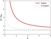Fig. 1. Electric conductivity σ as a function of κ, for the standard Kappa (red) and the modified Kappa (m-Kappa, blue-dotted) approaches, and normalized to the Maxwellian limit σM (which is reduced to the horizontal dashed line). The two Kappa-based functions approach the Maxwellian limit for κ → ∞ and diverge at the pole κ = 2.

3.2. The thermoelectric coefficient

The thermoelectric coefficient α was derived by setting E = 0 and ∇n = 0, which simplifies Eq. (20) to

$$\begin{array}{c}\hfill f_1=-\frac{f_{\kappa }(\kappa +1)}{{\nu }_{\mathrm{ei}}(k_{\mathrm{B}}T\eta +\epsilon )}\frac{\epsilon }{T}\mathrm{\nabla }T·\mathit{v}+\frac{3}{2}\frac{f_{\kappa }}{{\nu }_{\mathrm{ei}}}\frac{\mathrm{\nabla }T}{T}·\mathit{v}.\end{array}$$(28)

We inserted Eq. (28) into Eq. (10) and obtain

$$\begin{array}{cc}& \mathit{j}=\frac{(\kappa +1)e}{T}\mathrm{\nabla }T·{\displaystyle \int }{\mathrm{d}}^{3}v\frac{\mathit{v}\mathit{v}}{{\nu }_{\mathrm{ei}}}{(k_{\mathrm{B}}T\eta +\epsilon )}^{-1}\epsilon f_{\kappa }\hfill \\ \hfill & -\frac{3}{2}\frac{e}{T}\mathrm{\nabla }T·{\displaystyle \int }{\mathrm{d}}^{3}v\frac{\mathit{v}\mathit{v}}{{\nu }_{\mathrm{ei}}}{f}_{\kappa }\hfill \\ \hfill & =[\frac{(\kappa +1)e}{3T}\langle \frac{v^2\epsilon }{{\nu }_{\mathrm{ei}}}{(k_{\mathrm{B}}T\eta +\epsilon )}^{-1}\rangle -\frac{e}{2T}\langle \frac{v^2}{{\nu }_{\mathrm{ei}}}\rangle ]\mathrm{\nabla }T.\hfill \end{array}$$(29)

From Eqs. (29) and (8), we can identify the expression for α as

$$\begin{array}{cc}& \alpha =-\frac{(\kappa +1)e}{3\sigma T}\langle \frac{v^2\epsilon }{{\nu }_{\mathrm{ei}}}{(k_{\mathrm{B}}T\eta +\epsilon )}^{-1}\rangle +\frac{e}{2\sigma T}\langle \frac{v^2}{{\nu }_{\mathrm{ei}}}\rangle \hfill \\ \hfill & =-\frac{(\kappa +1)m^3}{24\pi \sigma k_{\mathrm{B}}{T}^{2}n\eta z{e}^3{L}_{\mathrm{ei}}}\langle v^7{(1+A_{\kappa }{v}^2)}^{-1}\rangle \hfill \\ \hfill & +\frac{m^2}{8\pi \sigma Tnz{e}^3{L}_{\mathrm{ei}}}\langle v^5\rangle .\hfill \end{array}$$(30)

Solving the integrals (see Appendix B) and inserting the expression for σ from Eq. (26) yields the final form of the thermoelectric coefficient

$$\begin{array}{c}\hfill \alpha =-\frac{\eta }{\kappa -3}\frac{5}{2}\frac{k_{\mathrm{B}}}{e},\end{array}$$(31)

with η = κ for the standard Kappa. For the modified Kappa approach (η = κ − 3/2), the result in Eq. (31) slightly differs from Eq. (22) in Du (2013), and this is due to the correction term in Eq. (20). A graphical comparison of Eq. (31) with the result in Du (2013) is shown in Appendix A. The Maxwellian limit (κ → ∞) takes the following form:

$$\begin{array}{c}\hfill {\alpha }_{\mathrm{M}}=-\frac{5}{2}\frac{k_{\mathrm{B}}}{e}.\end{array}$$(32)

In Fig. 2 the normalized thermoelectric coefficient is plotted as a function of the κ parameter for both Kappa approaches, the standard one (red line) and modified one (blue-dotted line), and these are compared to the Maxwellian limit (black-dashed line). Again, for the normalization, we used the same Maxwellian limit. For large κ → ∞, both Kappa approaches tend to be similar to the Maxwellian result, while for finite values of κ < 6 (but greater than pole at κ = 3), the standard Kappa approach (η = κ) yields markedly larger values of α (readers are encouraged to compare the red- and black-dashed lines and selected values in Table C.2. Instead, a modified Kappa underestimates the effects of suprathermals on α, as has resulted from a comparison of red- and blue-dotted lines, and the corresponding results in Table C.2.

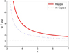Fig. 2. Thermoelectric coefficient α as a function of κ, for the standard Kappa (red) and the modified Kappa (m-Kappa, blue-dotted) approaches, and normalized to the Maxwellian limit αM (which is reduced to the horizontal dashed line). The two Kappa-based functions approach the Maxwellian limit for κ → ∞ and diverge at the pole κ = 3.

3.3. The thermal conductivity

For the evaluation of thermal conductivity (λ) in the absence of an electric current (j = 0), Eq. (8) becomes E = α ∇T, which we inserted into Eq. (20) (and set ∇n = 0) to obtain

$$\begin{array}{c}\hfill f_1=-\frac{f_{\kappa }(\kappa +1)(\alpha e+\epsilon /T)}{{\nu }_{\mathrm{ei}}(k_{\mathrm{B}}T\eta +\epsilon )}\mathrm{\nabla }T·\mathit{v}+\frac{3}{2}\frac{f_{\kappa }}{{\nu }_{\mathrm{ei}}}\frac{\mathrm{\nabla }T}{T}·\mathit{v}.\end{array}$$(33)

In Eq. (11), for the heat flux, the integral of the stationary f_κ vanishes (integrand is an odd function of v), and by substituting f₁ from Eq. (33), the heat flux becomes

$$\begin{array}{cc}& \mathit{q}=-(\kappa +1){\displaystyle \int }{\mathrm{d}}^{3}v\frac{\mathit{v}\mathit{v}}{{\nu }_{\mathrm{ei}}}\frac{(\alpha e+\epsilon /T)\epsilon f_{\kappa }}{k_{\mathrm{B}}T\eta +\epsilon }\mathrm{\nabla }T\hfill \\ \hfill & +\frac{3}{2T}{\displaystyle \int }{\mathrm{d}}^{3}v\frac{\mathit{v}\mathit{v}}{{\nu }_{\mathrm{ei}}}\epsilon f_{\kappa }\mathrm{\nabla }T\hfill \\ \hfill & =(-\frac{\kappa +1}{3}\langle \frac{v^2}{{\nu }_{\mathrm{ei}}}\frac{(\alpha e+\epsilon /T)\epsilon }{k_{\mathrm{B}}T\eta +\epsilon }\rangle +\frac{1}{2T}\langle \frac{v^2}{{\nu }_{\mathrm{ei}}}\epsilon \rangle )\mathrm{\nabla }T.\hfill \end{array}$$(34)

Comparing the coefficients of ∇T in Eqs. (34) and (9) allowed us to identify the thermal conductivity

$$\begin{array}{cc}& \lambda =\frac{\kappa +1}{3}\langle \frac{v^2}{{\nu }_{\mathrm{ei}}}\frac{(\alpha e+\epsilon /T)\epsilon }{k_{\mathrm{B}}T\eta +\epsilon }\rangle -\frac{1}{2T}\langle \frac{v^2}{{\nu }_{\mathrm{ei}}}\epsilon \rangle \hfill \\ \hfill & =\frac{(\kappa +1)\alpha m^3}{24\pi z{e}^3{k}_{\mathrm{B}}Tn\eta L_{\mathrm{ei}}}\langle v^7{(1+A_{\kappa }{v}^2)}^{-1}\rangle \hfill \\ \hfill & +\frac{(\kappa +1)m^4}{48\pi z{e}^4{k}_{\mathrm{B}}{T}^{2}n\eta L_{\mathrm{ei}}}\langle v^9{(1+A_{\kappa }{v}^2)}^{-1}\rangle \hfill \\ \hfill & -\frac{m^3}{16\pi z{e}^{4}nT{L}_{\mathrm{ei}}}\langle v^7\rangle ,\hfill \end{array}$$(35)

where the collision frequency from Eq. (18) was inserted. After solving the integrals in Eq. (35) (see Appendix B), we obtain the final expression for the thermal conductivity

$$\begin{array}{c}\hfill \lambda =\frac{\mathrm{\Gamma }(\kappa -4)}{\mathrm{\Gamma }(\kappa -1/2)}\frac{{\eta }^{7/2}}{(\kappa -3)}(16\kappa -8)\frac{\sqrt{2}{k}_{\mathrm{B}}{\left(k_{\mathrm{B}}T\right)}^{5/2}}{m^{1/2}{\pi }^{3/2}z{e}^4{L}_{\mathrm{ei}}},\end{array}$$(36)

with η = κ for the standard Kappa approach. For the modified Kappa (η = κ − 3/2), the expression obtained for λ differs from Eq. (26) in Du (2013) due to the additional middle term in Eq. (20). A graphical contrast from Eq. (36) to the result in Du (2013) is displayed in Appendix A. In this case, the Maxwellian limit (κ → ∞) takes the following form:

$$\begin{array}{c}\hfill {\lambda }_{\mathrm{M}}=\frac{16\sqrt{2}{k}_{\mathrm{B}}{\left(k_{\mathrm{B}}T\right)}^{5/2}}{m^{1/2}{\pi }^{3/2}z{e}^4{L}_{\mathrm{ei}}}.\end{array}$$(37)

Thermal conductivity is plotted in Fig. 3 as a function of κ, for both Kappa approaches, and normalized to the Maxwellian limit. While for very large values of κ → ∞, both Kappa approaches approach their Maxwellian limit, for finite and still large κ < 8 (but greater than the pole at κ = 4), the standard Kappa provides estimations of λ (red line) much greater than those obtained with a modified Kappa approach (blue-dotted line). By contrasting this to the Maxwellian limit (black-dashed line), we also find a significant contribution of suprathermal population to thermal conductivity. See also the corresponding results in Table C.3.

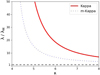Fig. 3. Thermal conductivity λ as a function of κ, for the standard Kappa (red) and the modified Kappa (m-Kappa, blue-dotted) approaches, and normalized to the Maxwellian limit λM (which is reduced to the horizontal dashed line). The two Kappa-based functions approach the Maxwellian limit for κ → ∞ and diverge at the pole κ = 4.

3.4. The diffusion coefficient

The diffusion coefficient D was obtained from Eq. (20) by setting both E = 0 and ∇T = 0, such that

$$\begin{array}{c}\hfill f_1=-\frac{f_{\kappa }}{{\nu }_{\mathrm{ei}}n}\mathrm{\nabla }n·\mathit{v}.\end{array}$$(38)

The particle flux from Eq. (12) simplifies to

$$\begin{array}{c}\hfill \mathbf{\Gamma }={\displaystyle \int }{\mathrm{d}}^{3}v\mathit{v}f={\displaystyle \int }{\mathrm{d}}^{3}v\mathit{v}{f}_1,\end{array}$$(39)

as the integral ∫d³v v f_κ vanishes. We inserted Eq. (38) into Eq. (39) to obtain

$$\begin{array}{c}\hfill \mathbf{\Gamma }=-\frac{1}{n}{\displaystyle \int }{\mathrm{d}}^{3}v\frac{\mathit{v}\mathit{v}}{{\nu }_{\mathrm{ei}}}{f}_{\kappa }\mathrm{\nabla }n=-\frac{1}{3n}\langle \frac{v^2}{{\nu }_{\mathrm{ei}}}\rangle \mathrm{\nabla }n,\end{array}$$(40)

and comparing the coefficients of ∇n in Eqs. (40) and Eq. (13) allowed us to identify the diffusion coefficient

$$\begin{array}{c}\hfill D=\frac{1}{3n}\langle \frac{v^2}{{\nu }_{\mathrm{ei}}}\rangle =\frac{m^2}{12\pi z{e}^4{L}_{\mathrm{ei}}{n}^2}\langle v^5\rangle .\end{array}$$(41)

The computation of the integral in Eq. (41) (see Appendix B) yields the final form of the diffusion coefficient

$$\begin{array}{c}\hfill D=\frac{\mathrm{\Gamma }(\kappa -3)}{\mathrm{\Gamma }(\kappa -1/2)}{\eta }^{5/2}\frac{4\sqrt{2}{(k_{\mathrm{B}}T)}^{5/2}}{{\pi }^{3/2}{m}^{1/2}z{e}^4{L}_{\mathrm{ei}}n},\end{array}$$(42)

with a singularity at κ = 3, and with η = κ for the standard Kappa and η = κ − 3/2 for the modified one. For κ → ∞, Eq. (42) leads to the Maxwellian limit

$$\begin{array}{c}\hfill D_{\mathrm{M}}=\frac{4\sqrt{2}{(k_{\mathrm{B}}T)}^{5/2}}{{\pi }^{3/2}{m}^{1/2}z{e}^4{L}_{\mathrm{ei}}n}.\end{array}$$(43)

Figure 4 displays the diffusion coefficient as a function of κ for both Kappa approaches, the standard (red line) and modified one (blue-dotted line). These are normalized to the Maxwellian limit (κ → ∞), which reduces to the horizontal dashed line. Similar to the previous results, we find the results from a modified Kappa approach (η = κ − 3/2) to decrease faster to the Maxwellian limit and to underestimate the diffusion coefficient overall, by comparison to the standard Kappa approach (η = κ). Values tabulated for the diffusion coefficient in Table C.4 may also help to understand these differences.

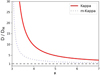Fig. 4. Diffusion coefficient D as a function of κ, for the standard Kappa (red) and the modified Kappa (m-Kappa, blue-dotted) approaches, and normalized to the Maxwellian limit αM (which is reduced to the horizontal dashed line). The two Kappa-based functions approach the Maxwellian limit for κ → ∞ and diverge at the pole κ = 3.

3.5. The mobility coefficient

The mobility coefficient μ was derived by setting ∇T = 0 and ∇n = 0 in Eq. (20), resulting in the expression for the electric conductivity σ in Eq. (21). Thus, we inserted Eq. (21) into Eq. (39) to obtain

$$\begin{array}{c}\hfill \mathbf{\Gamma }=-\frac{(\kappa +1)e}{3}\langle \frac{v^2}{{\nu }_{\mathrm{ei}}}{(k_{\mathrm{B}}T\eta +\epsilon )}^{-1}\rangle \mathit{E}.\end{array}$$(44)

This expression is similar to Eq. (23), containing the same integral. We can, therefore, write the mobility coefficient as

$$\begin{array}{c}\hfill \mu =\frac{\mathrm{\Gamma }(\kappa -2)}{\mathrm{\Gamma }(\kappa -1/2)}{\eta }^{3/2}\frac{4\sqrt{2}{(k_{\mathrm{B}}T)}^{3/2}}{{\pi }^{3/2}{m}^{1/2}z{e}^3{L}_{\mathrm{ei}}n},\end{array}$$(45)

which has the same pole, that is, κ = 2, as the electric conductivity σ. Again, η = κ yields the Olbertian, while η = κ − 3/2 yields the modified approach. For κ → ∞, we find the Maxwellian limit

$$\begin{array}{c}\hfill {\mu }_{\mathrm{M}}=\frac{4\sqrt{2}{(k_{\mathrm{B}}T)}^{3/2}}{{\pi }^{3/2}{m}^{1/2}z{e}^3{L}_{\mathrm{ei}}n}.\end{array}$$(46)

Figure 5 shows the mobility coefficient as a function of κ for both Kappa approaches, the standard (red line) and the modified one (blue-dotted line), normalized to the Maxwellian limit. The enhancement of μ in the presence of suprathermals (i.e., in the standard Kappa), but also the underestimates from a modified Kappa, are significant, as previously discussed in Fig. 1 for the electric conductivity σ. Selected values for μ are tabulated in Table C.5, and they make these differences obvious.

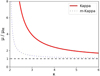Fig. 5. Mobility coefficient μ as a function of κ, for the standard Kappa (red) and the modified Kappa (m-Kappa, blue-dotted) approaches, and normalized to the Maxwellian limit αM (which is reduced to the horizontal dashed line). The two Kappa-based functions approach the Maxwellian limit for κ → ∞ and diverge at the pole κ = 2.

From Eqs. (26) and (45), we obtain the familiar relation between the electric conductivity and the mobility coefficient

$$\begin{array}{c}\hfill \sigma =ne\mu .\end{array}$$(47)

Furthermore, when combining Eqs. (42) and (45), we find the Einstein relation for charged particles

$$\begin{array}{c}\hfill D=\frac{\eta }{\kappa -3}\frac{\mu k_{\mathrm{B}}T}{e}.\end{array}$$(48)

For κ → ∞ this reduces to the familiar Einstein relation for charged particles for Maxwellian populations, that is, D_M = μ_M k_B T/e.

4. Conclusions and outlook

In the present paper we calculated transport coefficients in nonequilibrium plasmas and have shown the consequences of the presence of suprathermal particles on these coefficients. By assuming a plasma with Kappa-distributed electrons and using a particular expression for the collision frequency, we derived expressions for the electric conductivity σ, the thermoelectric coefficient α, the thermal conductivity λ, the diffusion coefficient D and the mobility coefficient μ. The results indicate significant enhancements in the transport coefficients in the presence of suprathermal particles. For the Kappa distribution, two common approaches are used in literature, the standard Kappa distribution originally introduced by Olbert (1968) and Vasyliūnas (1968), which enables a proper description of suprathermal populations in contrast to the quasi-thermal core, and a modified Kappa distribution, which does not have the same relevance (see Sect. 2). We computed the results for both Kappa approaches and have shown that the modified Kappa approach consistently underestimates the transport coefficients by comparison to the original Kappa approach at small values of κ, while the transport coefficients approach the Maxwellian limit for both Kappa variants. Furthermore, we were able to compare our results to those found earlier by Du (2013), who used the modified Kappa approach and whose results for the thermoelectric coefficient α and the thermal conductivity λ differ from our results due to a missing term in the derivation of the expression for the perturbed distribution function term (see Appendix A).

In the present analysis, we have not incorporated data from measurements or specific values for the temperature or associated quantities, but only evaluated normalized transport coefficients. For normalization, we used the Maxwellian limit that approaches the core of the Kappa distribution, and thus quantifies the contribution of the suprathermal electrons to the transport coefficients. Nonetheless, we have to point out that when using observational data, one needs to be cautious whether the measured temperature is after a Kappa fitting as the second-order velocity moment, or whether it is the lower one obtained after a Maxwellian fitting with the core of the observed distribution. In future work we plan to extend these evaluations of the transport coefficients for plasmas described by the regularized Kappa distribution (RKD; Scherer et al. 2017), which has been introduced to formulate a contradiction-free macroscopic description of nonthermal populations observed in the solar wind. By contrast to a standard Kappa, the RKD is defined for all values of κ > 0 and so are the macroscopic parameters, drift velocity, temperature, heat flux, etc., avoiding limitations corresponding to singularities (Lazar et al. 2020).

Acknowledgments

The authors acknowledge support from the Katholieke Universiteit Leuven and Ruhr-University Bochum. These results were obtained in the framework of the projects SCHL540201/35-1 (DFG-German Research Foundation), C14/19/089 (C1 project Internal Funds KU Leuven), G.0D07.19N (FWO-Vlaanderen), SIDC Data Exploitation (ESA Prodex-12), and Belspo projects BR/165/A2/CCSOM and B2/191/P1/SWiM.

References

Appendix A: Comments on the results in Du (2013)

In the derivation of the transport coefficients, we noticed a missing term in Eq. (10) in Du (2013) (readers are encouraged to compare this to Eq. (20) from the present paper). This term appears in both approaches and it is not clear why this term is left out in Du (2013), that is, whether it was overlooked in the derivation or neglected for simplification. While this has no effect on the electrical conductivity (σ) calculated in Du (2013), we obtain different results for the thermoelectric coefficient (α) and the thermal conductivity (λ) when considering the missing term.

In Du (2013), derivations are based on the modified Kappa approach, and the results are

$$\begin{array}{c}\hfill \alpha =-\frac{\kappa -3/2}{\kappa -3}4\frac{k_{\mathrm{B}}}{e},\end{array}$$(A.1)

which is slightly different from our Eq. (31) above for η = κ − 3/2, and

$$\begin{array}{c}\hfill \lambda =\frac{\kappa +1}{\kappa -3}\frac{\mathrm{\Gamma }(\kappa -4)}{\mathrm{\Gamma }(\kappa -1/2)}{(\kappa -\frac{3}{2})}^{7/2}\frac{16\sqrt{2}{k}_{\mathrm{B}}{\left(k_{\mathrm{B}}T\right)}^{5/2}}{m^{1/2}{\pi }^{3/2}z{e}^4{L}_{\mathrm{ei}}},\end{array}$$(A.2)

which is also different from our Eq. (36) above for η = κ − 3/2. These two expressions are plotted (green dash-dotted lines) in Figs A.1 and A.2, respectively, by contrast to our results. The results in Du (2013) differ from the values obtained in the present work for the modified Kappa approach (blue-dotted lines), and also from those obtained for a standard Kappa approach (red lines).

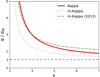Fig. A.1. Results for the thermoelectric coefficient α from Fig. 2 and those from Du (2013) for the modified Kappa approach (m-Kappa 2013, green dash-dotted line).

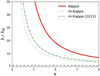Fig. A.2. Results for the thermal conductivity coefficient λ from Fig. 3 and those from Du (2013) for the modified Kappa approach (m-Kappa 2013, green dash-dotted line).

Appendix B: Integrals

The integrals occurring in Sec. 3 can be calculated by using substitution and integration by parts. Scherer et al. (2020) derived a general form to calculate integrals of type

$$\begin{array}{c}\hfill \langle v^n{(1+A_{\kappa }{v}^2)}^{\zeta }\rangle =4\pi N_{\kappa }{\displaystyle \underset{0}{\overset{\infty }{\int }}\mathrm{d}v{v}^{n+2}{(1+A_{\kappa }{v}^2)}^{\zeta -(\kappa +1)},}\end{array}$$(B.1)

using spherical coordinates and having already calculated the integrals over ϑ and ϕ. For the integrals, we then obtain the following expressions:

$$\begin{array}{cc}\hfill \langle v^5{(1+A_{\kappa }{v}^2)}^{-1}\rangle & =12\pi \frac{N_{\kappa }}{A_{\kappa }^4}\frac{\mathrm{\Gamma }(\kappa -2)}{\mathrm{\Gamma }(\kappa +2)},\hfill \end{array}$$(B.2)

$$\begin{array}{cc}\hfill \langle v^7{(1+A_{\kappa }{v}^2)}^{-1}\rangle & =48\pi \frac{N_{\kappa }}{A_{\kappa }^5}\frac{\mathrm{\Gamma }(\kappa -3)}{\mathrm{\Gamma }(\kappa +2)},\hfill \end{array}$$(B.3)

$$\begin{array}{cc}\hfill \langle v^9{(1+A_{\kappa }{v}^2)}^{-1}\rangle & =240\pi \frac{N_{\kappa }}{A_{\kappa }^6}\frac{\mathrm{\Gamma }(\kappa -4)}{\mathrm{\Gamma }(\kappa +2)},\hfill \end{array}$$(B.4)

$$\begin{array}{cc}\hfill \langle v^5\rangle & =12\pi \frac{N_{\kappa }}{A_{\kappa }^4}\frac{\mathrm{\Gamma }(\kappa -3)}{\mathrm{\Gamma }(\kappa +1)},\hfill \end{array}$$(B.5)

$$\begin{array}{cc}\hfill \langle v^7\rangle & =48\pi \frac{N_{\kappa }}{A_{\kappa }^5}\frac{\mathrm{\Gamma }(\kappa -4)}{\mathrm{\Gamma }(\kappa +1)}.\hfill \end{array}$$(B.6)

Appendix C: Tabulated transport coefficients

In this appendix we present a series of selected values of the normalized coefficients represented graphically in Figs. 1 – 5 in order to quantify the differences introduced by the suprathermals in the standard Kappa approach (subscript K) by comparison to the Maxwellian (subscript M), and also the underestimations from using a modified Kappa approach (subscript m-K).

The numbers in the tables clearly indicate the reinforcing effect on all transport coefficients by the presence of suprathermal particles represented by the original Kappa distribution f_K. For the electric conductivity σ (mobility coefficient μ, Tabs. C.1 and C.5) and the thermoelectric coefficient α (Tab. C.2), we find values 7 times the Maxwellian at κ = 2.5 and κ = 3.5, respectively. The contribution of suprathermal particles to the thermal conductivity λ (Tab. C.3) and the diffusion coefficient D (Tab. C.4) is even greater, and they manifest in values as large as about 18 to 150 times the Maxwellian for λ (at κ = 4.5 to 6) and about 10 to 20 times the Maxwellian for D (at κ = 3.5 to 4).

By comparing the original Kappa approach to the modified one (f_m − K), we identify an underestimation of all transport coefficients by the latter. Although the values of λ based on f_m − K are still relatively large (4 to 36 times the Maxwellian-based results) at values κ < 8, they are 2 to 4 times smaller than the results obtained with f_K. The results of the remaining transport coefficients reveal an even weaker contribution by suprathermal particles represented by f_m − K in comparison to the original Kappa approach, for example, for σ (μ) less than twice the Maxwellian at values for Kappa as small as κ = 2.5, and 4 times smaller than the f_K-based value. For α and D, the results obtained with f_m − K are less than twice the Maxwellian for κ ≳ 5, and again 2 to 4 times smaller than the numbers resulting from f_K.

All Tables

All Figures

	Fig. 1. Electric conductivity σ as a function of κ, for the standard Kappa (red) and the modified Kappa (m-Kappa, blue-dotted) approaches, and normalized to the Maxwellian limit σM (which is reduced to the horizontal dashed line). The two Kappa-based functions approach the Maxwellian limit for κ → ∞ and diverge at the pole κ = 2.
In the text

	Fig. 2. Thermoelectric coefficient α as a function of κ, for the standard Kappa (red) and the modified Kappa (m-Kappa, blue-dotted) approaches, and normalized to the Maxwellian limit αM (which is reduced to the horizontal dashed line). The two Kappa-based functions approach the Maxwellian limit for κ → ∞ and diverge at the pole κ = 3.
In the text

	Fig. 3. Thermal conductivity λ as a function of κ, for the standard Kappa (red) and the modified Kappa (m-Kappa, blue-dotted) approaches, and normalized to the Maxwellian limit λM (which is reduced to the horizontal dashed line). The two Kappa-based functions approach the Maxwellian limit for κ → ∞ and diverge at the pole κ = 4.
In the text

	Fig. 4. Diffusion coefficient D as a function of κ, for the standard Kappa (red) and the modified Kappa (m-Kappa, blue-dotted) approaches, and normalized to the Maxwellian limit αM (which is reduced to the horizontal dashed line). The two Kappa-based functions approach the Maxwellian limit for κ → ∞ and diverge at the pole κ = 3.
In the text

	Fig. 5. Mobility coefficient μ as a function of κ, for the standard Kappa (red) and the modified Kappa (m-Kappa, blue-dotted) approaches, and normalized to the Maxwellian limit αM (which is reduced to the horizontal dashed line). The two Kappa-based functions approach the Maxwellian limit for κ → ∞ and diverge at the pole κ = 2.
In the text

	Fig. A.1. Results for the thermoelectric coefficient α from Fig. 2 and those from Du (2013) for the modified Kappa approach (m-Kappa 2013, green dash-dotted line).
In the text

	Fig. A.2. Results for the thermal conductivity coefficient λ from Fig. 3 and those from Du (2013) for the modified Kappa approach (m-Kappa 2013, green dash-dotted line).
In the text

References

- Alexandrova, O., Chen, C. H. K., Sorriso-Valvo, L., Horbury, T. S., & Bale, S. D. 2013, Space Sci. Rev., 178, 101 [Google Scholar]
- Bale, S. D., Kasper, J. C., Howes, G. G., et al. 2009, Phys. Rev. Lett., 103, 211101 [NASA ADS] [CrossRef] [Google Scholar]
- Bale, S. D., Pulupa, M., Salem, C., Chen, C. H. K., & Quataert, E. 2013, ApJ, 769, L22 [Google Scholar]
- Balescu, R. 1988, Transport processes in plasmas - 1. Classical transport theory (Amsterdam: North Holland Publishing Company) [Google Scholar]
- Bhatnagar, P. L., Gross, E. P., & Krook, M. 1954, Phys. Rev., 94, 511 [Google Scholar]
- Bourouaine, S., Marsch, E., & Neubauer, F. M. 2011, A&A, 536, A39 [NASA ADS] [CrossRef] [EDP Sciences] [Google Scholar]
- Bourouaine, S., Alexandrova, O., Marsch, E., & Maksimovic, M. 2012, ApJ, 749, 102 [Google Scholar]
- Boyd, T. J. M., & Sanderson, J. J. 2003, The Physics of Plasmas (Cambridge: Cambridge University Press) [CrossRef] [Google Scholar]
- Braginskii, S. I. 1965, Rev. Plasma Phys., 1, 205 [Google Scholar]
- Collier, M. R., Hamilton, D. C., Gloeckler, G., Bochsler, P., & Sheldon, R. B. 1996, Geophys. Res. Lett., 23, 1191 [NASA ADS] [CrossRef] [Google Scholar]
- Du, J. 2013, Phys. Plasmas, 20, 092901 [NASA ADS] [CrossRef] [Google Scholar]
- Ebne Abbasi, Z., & Esfandyari-Kalejahi, A. 2019, Phys. Plasmas, 26, 012301 [CrossRef] [Google Scholar]
- Ebne Abbasi, Z., Esfandyari-Kalejahi, A., & Khaledi, P. 2017, Astrophys. Space Sci., 362, 103 [NASA ADS] [CrossRef] [Google Scholar]
- Goedbloed, H., Keppens, R., & Poedts, S. 2019, Magnetohydrodynamics of Laboratory and Astrophysical Plasmas (Cambridge: Cambridge University Press) [Google Scholar]
- Guo, R., & Du, J. 2019, Physica A, 523, 156 [NASA ADS] [CrossRef] [Google Scholar]
- Gurgiolo, C., Goldstein, M. L., Viñas, A. F., & Fazakerley, A. N. 2016, Ann. Geophys., 34, 1175 [NASA ADS] [CrossRef] [Google Scholar]
- Hagelaar, G. J. M., & Pitchford, L. C. 2005, Plasma Sources Sci. Technol., 14, 722 [NASA ADS] [CrossRef] [Google Scholar]
- Helander, P., & Sigmar, D. J. 2005, Collisional Transport in Magnetized Plasmas (Cambridge: Cambridge University Press) [Google Scholar]
- Lazar, M. 2017, Phys. Plasmas, 24, 034501 [NASA ADS] [CrossRef] [Google Scholar]
- Lazar, M., & Fichtner, H. 2021, in Kappa Distributions: From Observational Evidences via Controversial Predictions to a Consistent Theory of Nonequilibrium Plasmas, eds. M. Lazar, & H. Fichtner (Cham: Springer Nature) [CrossRef] [Google Scholar]
- Lazar, M., Poedts, S., & Schlickeiser, R. 2011, A&A, 534, A116 [NASA ADS] [CrossRef] [EDP Sciences] [Google Scholar]
- Lazar, M., Schlickeiser, R., & Poedts, S. 2012, in Exploring the Solar Wind, ed. M. Lazar (Rijeka: Intechopen Publishing), 241 [Google Scholar]
- Lazar, M., Poedts, S., & Michno, M. J. 2013, A&A, 554, A64 [NASA ADS] [CrossRef] [EDP Sciences] [Google Scholar]
- Lazar, M., Poedts, S., & Fichtner, H. 2015, A&A, 582, A124 [NASA ADS] [CrossRef] [EDP Sciences] [Google Scholar]
- Lazar, M., Fichtner, H., & Yoon, P. H. 2016, A&A, 589, A39 [NASA ADS] [CrossRef] [EDP Sciences] [Google Scholar]
- Lazar, M., Kim, S., López, R. A., et al. 2018, ApJ, 868, L25 [NASA ADS] [CrossRef] [Google Scholar]
- Lazar, M., Scherer, K., Fichtner, H., & Pierrard, V. 2020, A&A, 634, A20 [NASA ADS] [CrossRef] [EDP Sciences] [Google Scholar]
- Maksimovic, M., Pierrard, V., & Lemaire, J. F. 1997, A&A, 324, 725 [NASA ADS] [Google Scholar]
- Maksimovic, M., Zouganelis, I., Chaufray, J. Y., et al. 2005, J. Geophys. Res., 110, A09104 [NASA ADS] [Google Scholar]
- Marsch, E. 2006, Liv. Rev. Sol. Phys., 3, 1 [Google Scholar]
- Mason, G. M., & Gloeckler, G. 2012, Space Sci. Rev., 172, 241 [NASA ADS] [CrossRef] [Google Scholar]
- Matteini, L., Landi, S., Hellinger, P., et al. 2007, Geophys. Res. Lett., 34, L20105 [Google Scholar]
- Ogilvie, K. W., Geiss, J., Gloeckler, G., Berdichevsky, D., & Wilken, B. 1993, J. Geophys. Res., 98, 3605 [NASA ADS] [CrossRef] [Google Scholar]
- Olbert, S. 1968, Phys. Magnetos., 10, 641 [NASA ADS] [Google Scholar]
- Pierrard, V., & Lazar, M. 2010, Sol. Phys., 267, 153 [NASA ADS] [CrossRef] [Google Scholar]
- Pierrard, V., Lazar, M., & Schlickeiser, R. 2011, Sol. Phys., 269, 421 [NASA ADS] [CrossRef] [Google Scholar]
- Rat, V., André, P., Aubreton, J., et al. 2001, Phys. Rev. E, 64, 026409 [NASA ADS] [CrossRef] [Google Scholar]
- Roberts, D. A., & Miller, J. A. 1998, Geophys. Res. Lett., 25, 607 [NASA ADS] [CrossRef] [Google Scholar]
- Salem, C., Hubert, D., Lacombe, C., et al. 2003, ApJ, 585, 1147 [Google Scholar]
- Scherer, K., Fichtner, H., & Lazar, M. 2017, Europhys. Lett., 120, 50002 [NASA ADS] [CrossRef] [Google Scholar]
- Scherer, K., Husidic, E., Lazar, M., & Fichtner, H. 2020, MNRAS, 497, 1738 [NASA ADS] [CrossRef] [Google Scholar]
- Shaaban, S. M., Lazar, M., López, R. A., Fichtner, H., & Poedts, S. 2019, MNRAS, 483, 5642 [NASA ADS] [CrossRef] [Google Scholar]
- Shaaban, S. M., Lazar, M., López, R. A., & Poedts, S. 2020, ApJ, 899, 20 [NASA ADS] [CrossRef] [Google Scholar]
- Spatschek, K. H. 1990, Theoretische Plasmaphysik - Eine Einführung (Stuttgart: B. G. Teubner Verlag) [CrossRef] [Google Scholar]
- Štverák, Š., Trávniček, P., Maksimovic, M., et al. 2008, J. Geophys. Res., 113, 103 [Google Scholar]
- Vasyliūnas, V. M. 1968, J. Geophys. Res.: Space Phys., 73, 2839 [CrossRef] [Google Scholar]
- Viñas, A. F., Wong, H. K., & Klimas, A. J. 2000, ApJ, 528, 509 [CrossRef] [Google Scholar]
- Viñas, A. F., Moya, P. S., Navarro, R. E., et al. 2015, J. Geophys. Res.: Space Phys., 120, 3307 [CrossRef] [Google Scholar]
- Viñas, A. F., Gaelzer, R., Mace, R., Moya, P. S., & Araneda, J. A. 2017, in Kappa Distributions, ed. G. Livadiotis (Amsterdam: Elsevier) [Google Scholar]
- Vocks, C., Mann, G., & Rausche, G. 2008, A&A, 480, 527 [NASA ADS] [CrossRef] [EDP Sciences] [Google Scholar]
- Wang, L., & Du, J. 2017, Phys. Plasmas, 24, 102305 [NASA ADS] [CrossRef] [Google Scholar]
- Wilson, L. B., Koval, A., Szabo, A., et al. 2013, J. Geophys. Res., 118, 5 [NASA ADS] [CrossRef] [Google Scholar]
- Wilson, L. B., Chen, L. J., Wang, S., et al. 2019, ApJS, 243, 8 [NASA ADS] [CrossRef] [Google Scholar]
- Yoon, H. P., Rhee, T., & Ryu, C. M. 2006, J. Geophys. Res., 111, A09106 [NASA ADS] [Google Scholar]
- Zouganelis, I., Meyer-Vernet, N., Landl, S., Maksimovic, M., & Pantellini, F. 2005, ApJ, 626, L117 [NASA ADS] [CrossRef] [Google Scholar]