| Issue |
A&A
Volume 657, January 2022
|
|
|---|---|---|
| Article Number | A58 | |
| Number of page(s) | 8 | |
| Section | Stellar structure and evolution | |
| DOI | https://doi.org/10.1051/0004-6361/202141608 | |
| Published online | 10 January 2022 | |
Broad-band analysis of X-ray pulsar 2S 1845–024
1
Department of Physics and Astronomy, University of Turku, 20014 Turku, Finland
e-mail: armin.nabizadeh@utu.fi
2
Space Research Institute of the Russian Academy of Sciences, Profsoyuznaya Str. 84/32, Moscow 117997, Russia
3
School of Physics and Astronomy, Sun Yat-Sen University, Zhuhai, Guangdong 519082, PR China
4
Nordita, KTH Royal Institute of Technology and Stockholm University, 10691 Stockholm, Sweden
Received:
21
June
2021
Accepted:
12
October
2021
We present the results of a detailed investigation of the poorly studied X-ray pulsar 2S 1845−024 based on data obtained at the NuSTAR observatory during the type I outburst in 2017. Neither pulse phase-averaged nor phase-resolved spectra of the source show evidence for a cyclotron absorption feature. We also used data obtained from other X-ray observatories (Swift, XMM-Newton and Chandra) to study the spectral properties as a function of orbital phase. The analysis reveals a high hydrogen column density for the source reaching ∼1024 cm−2 around periastron. Using high-quality Chandra data we were able to obtain an accurate localization of 2S 1845−024 at RA = 18h48m16.s8 and Dec = −2°25′25.″1 (J2000), which allowed us to use infrared (IR) data to roughly classify the optical counterpart of the source as an OB supergiant at a distance of ≳15 kpc.
Key words: accretion, accretion disks / magnetic fields / pulsars: individual: 2S 1845–024 / stars: neutron / X-rays: binaries
© ESO 2022
1. Introduction
2S 1845−024 (also known as GS 1843−024) is a transient X-ray source discovered with the Ginga observatory (Makino & GINGA Team 1988; Koyama et al. 1990a). It belongs to the class of high-mass X-ray binaries (HMXBs). Many of the physical properties of the system and the neutron star (NS) are still unknown. The system contains an X-ray pulsar (XRP) with a spin period Pspin = 94.8 s (Makino & GINGA Team 1988; Zhang et al. 1996). A series of the Burst and Transient Source Experiment (BATSE) observations performed in 1991−1997 detected ten type I outbursts revealing an orbital period Porbital = 242.18 ± 0.01 d for the system (Finger et al. 1999). More outbursts around periastron passage (orbital phase zero) were detected later by different observatories (e.g., Doroshenko et al. 2008). No type II outbursts have yet been detected from the source. The timing analysis allows the orbital parameters of the system to be determined: the high eccentricity of e = 0.879 ± 0.005 and the projected semi-major axis ax sin i = 689 ± 38 lt-s, suggesting a high-mass companion (M > 7 M⊙) for 2S 1845−024 (Finger et al. 1999; Koyama et al. 1990a).
The companion star in this system has not yet been directly identified. However, the source is classified as a transient Be/XRP based on the outburst pattern and the highly eccentric orbit (Koyama et al. 1990a; Zhang et al. 1996; Finger et al. 1999). In addition, the location of the source in the Corbet (1986) diagram is consistent with a Be/NS binary. The 2−38 keV X-ray spectrum of 2S 1845−024, obtained by the Ginga Large Area Counter (LAC), fitted by a power law with a high-energy cutoff model, revealed a large hydrogen column density NH ≃ (1.5 − 3.0)×1023 cm−2 in the direction of the source (Koyama et al. 1990a). Assuming that the lower limit on NH is accounted for by the interstellar medium, Koyama et al. (1990a) estimated the source distance to be about 10 kpc. We emphasize that there is no Gaia distance measurements available for this source.
The BATSE observations of 2S 1845−024 also measured a secular long-term spin-up trend at a rate of  Hz s−1 during the 1991−1997 period of activity (Finger et al. 1999). Currently, however, the observations provided with the Fermi Gamma-ray Burst Monitor (GBM) Accreting Pulsars Program (GAPP1; Malacaria et al. 2020) show that the source has been in a spin-down phase during the last six years. It can therefore be inferred that the source underwent a torque reversal before entering to the long-term spin-down trend with a rate of
  Hz s−1 (Malacaria et al. 2020). Because there are no data available for the source in the period between 51560 and 56154 MJD, Malacaria et al. (2020) estimated that the torque reversal occurred at 53053 ± 250 MJD by extrapolating the spin-up and spin-down log-term trends in the gap between BATSE and GBM observations.
Although there are several X-ray observations available for 2S 1845−024, the properties of the source in the soft and hard X-ray bands have not been fully investigated. Namely, fundamental parameters such as the NS magnetic field strength, the type of the companion star, and the distance to the system have not yet been determined or are still debated. In the study presented here, we used a single NuSTAR observation, which was performed during a normal type I outburst on 2017 April 14 as well as several other archival observations obtained with different X-ray satellites to perform a detailed temporal and spectral analysis of 2S 1845−024 in a wide energy band in order to determine its properties.
2. Observations and data reduction
Since its discovery, 2S 1845−024, has been extensively observed by several instruments such as NuSTAR, XMM-Newton, Chandra, and Swift. The summary of the observations used in this work is given in Table 1. Here we focus on the details of the observations obtained by the mentioned X-ray observatories which were performed at different orbital phases (see Fig. 1), calculated using ephemeris TPeriastron = 2449616.98 ± 0.18 (JD) (Finger et al. 1999). The temporal and spectral analysis was done using HEASOFT 6.282 and XSPEC 12.11.1b3. For the spectral analysis, the data were grouped to have at least 25 counts per energy bin in order to use χ2 statistics unless otherwise stated in the text.
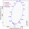 |
Fig. 1. Orbital phases corresponding to the date of each observation performed by NuSTAR, XMM-Newton, Chandra, and Swift/XRT. |
Observation log of 2S 1845−024.
2.1. NuSTAR observations
The NuSTAR X-ray observatory consists of two identical and independent co-aligned X-ray telescopes focusing the incident X-rays into two focal plane modules A and B (FPMA and FPMB) (Harrison et al. 2013). The instruments contain four (2 × 2) solid-state cadmium zinc telluride (CdZnTe) pixel detectors operating in a wide energy range of 3−79 keV. NuSTAR instruments provide an X-ray imaging resolution of 18″ full width at half maximum (FWHM) and a spectral energy resolution of 400 eV (FWHM) at 10 keV. 2S 1845−024 was observed with NuSTAR on 2017 April 14 for a duration of ∼35 ks during the peak of the outburst. In order to reduce the raw data, we followed the standard procedure explained in NuSTAR official user guides4 the NuSTAR Data Analysis Software NUSTARDAS v2.0.0 with a CALDB version 20201130. The source and background photons were extracted from circular regions with radii 90″ and 150″, respectively, for both modules.
2.2. Swift observations
2S 1845−024 was observed by the XRT telescope (Burrows et al. 2005) onboard the Neil Gehrels Swift Observatory (Swift; Gehrels et al. 2004) several times in the period of 2007–2019. In this study, we used five Swift/XRT observations, all obtained in the photon counting (PC) mode as listed in Table 1. The corresponding spectra were extracted using the online tools5 (Evans et al. 2009) provided by the UK Swift Science Data Centre. Because the count rate in all Swift observations is below 0.3 count s−1, the data were not affected by the pile-up effect6. One of the Swift/XRT observations (ObsID 00088089001) was performed simultaneously with the NuSTAR observation allowing us to obtain spectral parameters in a wider energy band 0.3−79 keV. The source spectra as observed by Swift/XRT and NuSTAR/FPMA-B were then fitted simultaneously in the energy ranges 0.3−10 and 4−79 keV, respectively, accounting for differences in normalization.
2.3. XMM-Newton observations
The X-ray Multi-Mirror Mission (XMM-Newton) (Jansen et al. 2001) carries three X-ray telescopes each with a medium spectral resolution European Photon Imaging Camera at the focus operating in the range of 0.2−10 keV (EPIC-MOS1, -MOS2 and -pn). 2S 1845−024 was observed by XMM-Newton two times in 2006 with the exposure times of ∼23 and ∼16 ks with all three EPIC X-ray instruments. We reduced and analyzed the data following the standard procedure explained in Science Analysis System (SAS) user guide7 using the software SAS version 17.0.0 and the latest available calibration files. We extracted the source spectra and light curves from a source-centered circular region with a radius of 20″ for all three instruments. The background was likewise extracted from source-free regions of the same radius in the same chips. We note that there are no MOS1 data available for observation ObsID 0302970601.
2.4. Chandra observations
2S 1845−024 was observed by the Chandra advanced CCD Imaging Spectrometer (ACIS) several times in 2002 and 2009 (see Table 1) providing a total exposure time of 55.4 ks. In all observations, the source is located in ACIS-S3 except for the observation ObsID 10512 in which the detector ACIS-I3 was used. Following the standard pipeline procedure8, we reprocessed the data to extract new event files (level 2) using the task CHANDRA_REPRO from the software package CIAO v4.12 with an up-to-date CALDB v4.9.1. We then extracted the source and background spectra from circular regions of 10″ and 30″ in radius, respectively.
2.5. UKIDSS/UKIRT observations
In order to study the type of companion star in 2S 1845−024 using the methods explained in Karasev et al. (2015) and Nabizadeh et al. (2019), the magnitudes of the star in two near-infrared (NIR) filters H and K are required. We took the magnitude of the counterpart in the K filter from the latest public release of the UKIRT Infrared Deep Sky Survey (UKIDSS) catalog UKIDSS/GPS DR11 PLUS9. However, the magnitude of the source in the H filter is not present in that catalog. To solve this problem, we performed an additional photometric analysis of UKIDSS image data (id 4543927 observed on 2006 June 12) using PSF-photometry (DAOPHOT II10) methods.
Having obtained the instrumental magnitudes of all the stars in the 3′ vicinity of 2S 1845−024, we were able to compare these instrumental magnitudes with those in the standard UKIDSS catalog (HAperMag3). We then selected only the stars brighter than 17 mag in the H-filter for this analysis, excluding overexposed objects. Thus, we estimated a mean correction value and converted the DAOPHOT magnitude (in the H-filter) of the probable counterpart into the real or observed magnitude in the corresponding filter (see Table 2). We emphasize that 2S 1845−024 is not detected in the J filter.
Coordinates and IR magnitudes of the counterpart of 2S 1845−024 based on UKIDSS/GPS and Spitzer data.
3. Analysis and results
3.1. Pulse profile and pulsed fraction
For the timing analysis, we used NuSTAR barycentric-corrected and background-subtracted light curves. The binary motion correction was also applied to the light curves to convert the observed time to the binary-corrected time using the orbital parameters obtained from Finger et al. (1999) and given in Table 3. The long exposure time and high count rate allowed us to determine the spin period of the NS of Pspin = 94.7171(3) s. To obtain the spin period and its uncertainty, the standard EFSEARCH procedure from the FTOOL package was applied on 103 simulated light curves created by using the count rates and uncertainties of the original 3−79 keV light curve (see e.g., Boldin et al. 2013). Considering the wide energy range of NuSTAR, we were able to study the pulse profile of the source as a function of energy. For this, we first extracted the source and background light curves in five energy bands 3−7, 7−18, 18−30, 30−50, and 50−79 keV. We then combined the light curves extracted from the modules FPMA and FPMB in order to increase the statistics.
Orbital parameters of 2S 1845−024 (Finger et al. 1999).
The energy-dependent light curves were folded with the obtained pulse period using the task EFOLD from the XRONOS package. Evolution of the pulse profile with energy is shown in the top five panels of Fig. 2. Pulse profiles demonstrate a complicated structure consisting of multiple peaks. The main maximum and minimum are around 0.1−0.2 and 0.6−0.7, respectively, where the zero phase is chosen arbitrarily. As can be seen, the pulse profile depends on energy, with the multi-peak structure becoming more prominent at higher energies. The most significant changes take place around the main minimum and maximum of the profile. This is best illustrated with the hardness ratio constructed using the pulse profiles in 3−7 and 18−30 keV bands as shown in the bottom panel of Fig. 2. The hardness ratio shows two clear hardenings of the emission at the rising part of the main maximum and at the center of the main minimum.
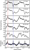 |
Fig. 2. Top panels: pulse profile of 2S 1845−024 in different energy bands obtained from the NuSTAR observation. Fluxes are normalized by the mean flux in each energy range. The red and blue dashed lines show the main maximum and minimum in the 3−7 keV band, respectively. The black dotted lines in the uppermost panel show the phase segments used to extract the phase-resolved spectra. Bottom panel: hardness ratio of the source over the pulse phase calculated as a ratio of normalized count rates in the pulse profiles in the energy bands 18−30 and 3−7 keV. The hardness ratio of unity is indicated by the horizontal blue solid line. |
We also calculated the pulsed fraction, determined as PF = (Fmax − Fmin)/(Fmax + Fmin), where Fmax and Fmin are the maximum and minimum fluxes of the pulse profile, as a function of energy. In the majority of XRPs, the pulse fraction shows a positive correlation with the energy (Lutovinov & Tsygankov 2009); however, as shown in Fig. 3, the pulsed fraction in 2S 1845−024 has values of around 40%−50% with no prominent dependence on the energy.
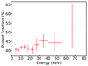 |
Fig. 3. Energy dependence of the pulse fraction of 2S 1845−024 obtained from the NuSTAR observation. |
3.2. Phase-averaged spectroscopy
The simultaneous observations of 2S 1845−024 obtained with Swift/XRT and NuSTAR allowed us to perform the spectral analysis in a broad band, 0.3−79 keV, for the first time for the source. The broadband spectrum of 2S 1845−024 shown in Fig. 4 was found to have a shape typical for XRPs (Filippova et al. 2005). According to Koyama et al. (1990a), the source continuum can be fitted by a phenomenological model such as a power law with a high-energy exponential cut-off. However, to find the best-fit model, we tested several continuum models as listed in Table 4. Consequently, the FDCUT model could not fit the spectrum, while CUTOFFPL, NPEX, and COMPTT gave acceptable fits with χ2 (d.o.f.) of 2098 (1769), 1787 (1766), and 2007 (1768), respectively. The model PO × HIGHECUT fitted the spectrum slightly better with χ2 (d.o.f.) = 1769 (1767). Therefore, and also to be able to make a comparison between our results and the previous studies, we used this preferred model for both the phase-averaged and the phase-resolved analysis. The Galactic and intrinsic absorption was modeled using photoelectric absorption model TBABS with abundances from Wilms et al. (2000) and atomic cross-sections adopted from Verner et al. (1996). We also used a Gaussian emission component to account for the narrow fluorescent iron line at 6.4 keV.
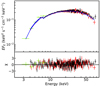 |
Fig. 4. Top panel: broad band X-ray spectrum of 2S 1845−024 extracted from Swift/XRT (green crosses) and NuSTAR/FPMA and FPMB (red and black crosses). The solid blue line represents the best-fit model CONSTANT × TBABS × (PO × HIGHECUT + GAU). Bottom panel: residuals from the best-fit model in units of standard deviations. We emphasize that the Swift/XRT spectrum is obtained in the range 0.3−10 keV; however, there are not enough soft X-ray photons below 3 keV because the spectrum is highly absorbed. |
Phenomenological models used to fit the source spectral continuum.
The best-fit composite model (CONSTANT × TBABS (PO × HIGHECUT + GAUSSIAN)) along the data and the corresponding residuals are shown in Fig. 4 and the best-fit parameters and the corresponding uncertainties at 68.3% (1σ) confidence level are given in Table 5. The fit revealed a large hydrogen column density NH = (22.7 ± 0.7)×1022 cm−2. We note that the Galactic mean value in the direction of the source is 1.81 × 1022 cm−2 (Willingale et al. 2013) which is significantly lower than what we obtained. This discrepancy could be due to a significant intrinsic absorption in the system. To explore this hypothesis, we studied variations of the column density as a function of orbital phase.
Best-fit parameters for the joint Swift/XRT and NuSTAR phase-averaged spectrum approximated with the CONSTANT × TBABS (POWERLAW × HIGHECUT + GAUSSIAN) model.
We used the 11 archival observations (see Table 1) performed at different orbital phases as listed in Table 6. As the data cover only the soft X-ray band below 10 keV, we modeled the spectra using a simple composite model TBABS × (PO + GAUSSIAN). We note that the NuSTAR spectra were also fitted using the same model in the energy range 4−10 keV. Due to the lack of high count statistics in some observations we were unable to detect the iron emission line and therefore fixed the line centroid energy and width to our best-fit values from the joint Swift+NuSTAR data. We thus obtained the column density for different orbital phases, and present these in Table 6. The corresponding X-ray flux for each observation was also calculated in the energy range 0.3−10 keV and is reported in the same table. The data show a strong dependence of NH on the orbital phase as well a correlation with the flux (see Table 6). For those observations with lower exposure time, we binned the spectra to have at least 1 count s−1 and used W-statistics (Wachter et al. 1979) in order to get more reliable fits.
Spectral parameters of 2S 1845−024 as a function of orbital phase.
We emphasize that the best-fit model showed no evidence of a cyclotron resonant scattering feature (CRSF) in the broad-band source spectra (see Fig. 4). However, we continued searching for the possible cyclotron line following the steps explained by Doroshenko et al. (2020). Nevertheless, we did not detect any absorption feature at any energy with significance above ∼2.4σ.
3.3. Phase-resolved spectroscopy
Phase-resolved spectroscopy is a useful technique for studying the spatial properties of the emitting region of the NS. Based on the good counting statistics, we extracted 20 equally spaced phase bins (see upper panel in Fig. 2) from the available NuSTAR observation of 2S 1845−024. Each spectrum was fitted with our best-fit model (CONSTANT × TBABS (PO × HIGHECUT + GAUSSIAN); see Sect. 3.2). Similar to the phase-average spectral analysis, we fixed the iron line width at 0.1 keV for all 20 spectra. The evolution of the fit parameters are shown in Fig. 5.
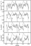 |
Fig. 5. Variations of the spectral parameters of the best-fit model as a function of pulse phase. The black crosses from the uppermost to the lowest panel show: neutral hydrogen column density NH in units of 1022 cm−2, photon index, cutoff energy, and folding energy. The full energy (3−79 keV) averaged pulse profile of the source is shown in gray in each panel. Errors are 1σ. |
The hydrogen column density NH varies in the range of (15−31) × 1022 cm−2 showing a marginally significant deviation from a constant. The photon index Γ shows a similar behavior to that of NH, varying from ∼0.7 at the main maximum to ∼1.5 at the second minimum of the pulse. The cutoff energy Ecut remains almost constant around 8 keV throughout the pulse with variations between 5.8 and 9.5 keV. The folding energy Efold is more variable reaching ∼48 keV near the second minimum of the pulse and decreasing down to 19 keV at the main maximum.
Because there is a possible strong internal correlation between NH and Γ in the soft X-ray band, we constructed the confidence contour plot of these two parameters using the spectra of the phases 0.5 and 0.8 where these parameters have different values (see Fig. 6). We see that although the values of NH for two phases agree within 2σ confidence level, the photon index is significantly different, pointing to the intrinsic variability of the spectrum.
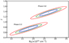 |
Fig. 6. Confidence contours of NH versus Γ obtained using the best-fit model for the spin phase-resolved spectra at phases 0.5 and 0.8 (see the text). The blue, green, and red contours correspond to the 1σ, 2σ, and 3σ confidence levels obtained using χ2 statistics for two free parameters. |
3.4. X-ray position and IR companion
Due to the poor localization of 2S 1845−024, the nature of the optical counterpart in this system remains unclear. 2S 1845−024 is located in the Scutum region which is crowded by transient XRPs and their companions (Koyama et al. 1990b). In order to determine the source position from the X-ray data, we selected one of the Chandra observations (ObsID 2689). Using the task CELLDETECT standard routines11, we obtained the source position at RA = 18 and Dec =
  (J2000). A total uncertainty of 1″ (at 90% confidence level radius), including the systematic uncertainty of Chandra absolute positions12, was obtained for the localization accuracy of the source.
We also obtained the astrometrically corrected source coordinates from the averaged image of all available Swift/XRT observations using the online XRT products generator13. Based on this, the source is located at RA = 18 and Dec =
  (J2000) with an error radius of
  at 90% confidence level, which is fully consistent with the Chandra results (see Fig. 7).
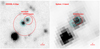 |
Fig. 7. Images of the sky around 2S 1845−024 in the K-filter obtained by the UKIRT telescope (GPS/UKIDSS sky survey, left) and in the 3.6μ-band obtained by the Spitzer telescope (right). The red circles indicate an uncertainty for the source position based on the Swift (dashed line) and Chandra (solid line) data, respectively. Cyan contours mark two IR objects closest to the X-ray position. |
3.5. Nature of the IR companion
Using the results of Chandra localization and data of the UKIDSS NIR sky survey, we were able to identify the IR counterpart of 2S 1845−024 (see Fig. 7, left panel). The coordinates and magnitudes of the IR counterpart are given in Table 2. The expected class of the star as well as its distance can be estimated using a method that has been successfully applied in a number of sources (see, e.g., Karasev et al. 2015; Nabizadeh et al. 2019).
Comparing the measured color of the source, (H − K) = 2.30 ± 0.05, with the intrinsic colors (H − K)0 of different classes of stars (Wegner 2014, 2015, all values were converted into the UKIRT filter system via relations from Carpenter 2001), we can estimate the corresponding extinction corrections E(H − K) = (H − K)−(H − K)0. 2S 1845−024 is located far from the Galactic bulge, and therefore we can use a standard extinction law (Cardelli et al. 1989) to transform each E(H − K) into the extinction AK. In turn, comparing absolute magnitudes of the same classes of stars MK (Wegner 2000, 2006, 2007) with the measured magnitude of the source in the K-filter, we are able to estimate a probable distance D to each class of stars by solving 5 − 5log10D = MK − K + AK. The results of this approach are indicated in Fig. 8.
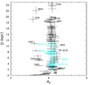 |
Fig. 8. Distance–extinction diagram showing how far away the star (black dots for normal and cyan for Be stars) of a specific class should be located if it is a counterpart of 2S 1845−024 and the appropriate extinction towards such a star. |
Unfortunately, having magnitudes only in two filters makes it challenging to draw any solid conclusions about the nature of the IR companion. However, the extinction AK towards the system can be roughly estimated. According to Fig. 8, AK ≃ 4.1 accounts for OB stars, including giants and supergiants, and AK ≃ 3.7 for red giants. By converting these extinction magnitudes into the hydrogen column density NH using the standard relations AV = 8.93 × AK (Cardelli et al. 1989) and NH = 2.87 × 10²¹ × AV (Foight et al. 2016), we obtain NH ≃ (10 − 11)×1022 cm−2 for different types of the companion stars. At the same time, the X-ray spectrum revealed a significantly higher column density of 22.7 × 1022 cm−2, which is typical for highly absorbed HMXB systems (see, e.g., Rahoui et al. 2008). This circumstance may indicate that 2S 1845−024 belongs to this class of binary system.
To clarify the nature of the companion, we also used the mid-IR data obtained by the Spitzer telescope14 (see Table 2). However, as can be seen from Fig. 7, there is another star located near the probable IR counterpart of 2S 1845−024. The spatial resolution of Spitzer did not allow us to fully resolve these objects (see cyan contours in Fig. 7), and therefore we were not able to exclude that the resulting mid-IR fluxes mentioned in Table 2 are affected by the confusion of these two stars.
Nevertheless, if we assume an OB supergiant (B9Iab, B5Iab, O5Ia etc.) to be the counterpart of 2S 1845−024, the distance to the source is expected to be more than ∼16 kpc (see Fig. 8). This is in line with the findings of Koyama et al. (1990a) who estimated a distance to the source of 10 kpc based on the high NH value in the source spectrum. Our spectral analysis also supports these results as NH shows variations on the orbital timescale from ∼(1–2) × 1023 cm−2 at the phase around 0.5 to ∼1024 cm−2 around the periastron passage. The lowest value of NH is almost an order of magnitude higher than the Galactic mean value in the direction of the source. This fact along with a positive correlation of the NH value with the X-ray flux points to the presence of a strong stellar wind in the system. Similar behavior is observed in other XRPs with hypergiant optical companions (e.g., for GX 301–2, Islam & Paul 2014). However, at the same time, we cannot rule out that the companion star is of another class. Thus, to reliably establish the nature of the IR companion of 2S 1845−024, spectroscopic observations in the near-IR band are required, for example with K-band spectroscopy. When the class of the companion star is established, we will be able to use the diagram shown in Fig. 8 to estimate the distance to the source with high accuracy.
4. Discussion and conclusions
In this work, we present the results of the detailed X-ray and IR analysis of the poorly studied XRP 2S 1845−024 and its companion during the type I outburst of the source in 2017. For X-ray analysis, we used a single NuSTAR observation performed during the outburst and several X-ray observations obtained by XMM-Newton, Chandra, and Swift. For the IR analysis, data obtained from UKIDSS/GPS and Spitzer/GLIMPSE surveys were used.
In order to determine the magnetic field strength of the NS in the system, which was one of our primary goals, we searched for a possible cyclotron absorption line in the broad-band NuSTAR spectrum. Such a feature was not discovered in phase-averaged or in phase-resolved spectra of 2S 1845−024. Therefore, it can be inferred that either the line does not exist in the considered energy range or it is too weak to be detected with the current sensitivity of the observations. In the former case, considering the lower and upper limits of the operating energy-band of the NuSTAR instruments, we only can estimate the magnetic field strength of the source to be either weaker than ∼4 × 10¹¹ G or stronger than ∼7 × 10¹² G. Further sensitive observations are required to come to any solid conclusions.
In order to determine the nature of the companion and the distance to 2S 1845−024, we analyzed the IR data. However, the availability of the magnitudes only in two (H and K) filters limited us to roughly classifying the IR-companion in 2S 1845−024 as an OB-supergiant star located at a distance of more than ∼16 kpc. To establish a more accurate estimation of the nature of the IR companion in this system, as well as the distance to the source, sensitive spectroscopic observations in the near-IR band (e.g., K-band spectroscopy) are required. Our conclusion about the class of the optical companion is in agreement with the X-ray spectral properties of the source. The good coverage of the binary orbit with observations in the soft X-rays allowed us to investigate the variation of column density NH as a function of orbital phase, which revealed the presence of a strong stellar wind in the system. However, we emphasize that an extensive study of the iron line is required to support this interpretation (see Islam & Paul 2014).
An estimation of the distance to 2S 1845−024 could also be obtained using the observed fluxes and presumable luminosity of the source in the different states. In particular, in the low state when the observed flux drops to about 10−12 erg s−1 cm−2 (see Table 6), one can expect the luminosity of the source to be above ∼1034 erg s−1 in the case of the ongoing accretion (Tsygankov et al. 2017, 2019) and, therefore, the distance to the system cannot be below ∼10 kpc. From another viewpoint, the peak luminosity during type-I outbursts from the transient XRPs can be of the order of 1037 erg s−1. Taking into account the maximal observed flux from 2S 1845−024 of around 10−9 erg s−1 cm−2 one can estimate the upper limit on the distance as ∼15 kpc. These rough estimates agree with results obtained from the IR data.
Acknowledgments
This work was supported by the grant 14.W03.31.0021 of the Ministry of Science and Higher Education of the Russian Federation. We also acknowledge the support from the Finnish Cultural Foundation through project number 00200764 and 85201677 (AN), the Academy of Finland travel grants 317552, 322779, 324550, 331951, and 333112, the National Natural Science Foundation of China grants 1217030159, 11733009, U2038101, U1938103, and the Guangdong Major Project of the Basic and Applied Basic Research grant 2019B030302001 (LJ). This work is based in part on data of the UKIRT Infrared Deep Sky Survey. Also, part of this work is based on observations made with the Spitzer Space Telescope, which is operated by the Jet Propulsion Laboratory, California Institute of Technology under a contract with NASA.
References
- Boldin, P. A., Tsygankov, S. S., & Lutovinov, A. A. 2013, Astron. Lett., 39, 375 [NASA ADS] [CrossRef] [Google Scholar]
- Burrows, D. N., Hill, J. E., Nousek, J. A., et al. 2005, Space Sci. Rev., 120, 165 [Google Scholar]
- Cardelli, J. A., Clayton, G. C., & Mathis, J. S. 1989, ApJ, 345, 245 [Google Scholar]
- Carpenter, J. M. 2001, AJ, 121, 2851 [Google Scholar]
- Corbet, R. H. D. 1986, MNRAS, 220, 1047 [NASA ADS] [CrossRef] [Google Scholar]
- Doroshenko, V. A., Doroshenko, R. F., Postnov, K. A., Cherepashchuk, A. M., & Tsygankov, S. S. 2008, Astron. Rep., 52, 138 [NASA ADS] [CrossRef] [Google Scholar]
- Doroshenko, V., Tsygankov, S., Long, J., et al. 2020, A&A, 634, A89 [NASA ADS] [CrossRef] [EDP Sciences] [Google Scholar]
- Evans, P. A., Beardmore, A. P., Page, K. L., et al. 2009, MNRAS, 397, 1177 [Google Scholar]
- Filippova, E. V., Tsygankov, S. S., Lutovinov, A. A., & Sunyaev, R. A. 2005, Astron. Lett., 31, 729 [NASA ADS] [CrossRef] [Google Scholar]
- Finger, M. H., Bildsten, L., Chakrabarty, D., et al. 1999, ApJ, 517, 449 [NASA ADS] [CrossRef] [Google Scholar]
- Foight, D. R., Güver, T., Özel, F., & Slane, P. O. 2016, ApJ, 826, 66 [Google Scholar]
- Gehrels, N., Chincarini, G., Giommi, P., et al. 2004, ApJ, 611, 1005 [Google Scholar]
- Harrison, F. A., Craig, W. W., Christensen, F. E., et al. 2013, ApJ, 770, 103 [Google Scholar]
- Islam, N., & Paul, B. 2014, MNRAS, 441, 2539 [NASA ADS] [CrossRef] [Google Scholar]
- Jansen, F., Lumb, D., Altieri, B., et al. 2001, A&A, 365, L1 [NASA ADS] [CrossRef] [EDP Sciences] [Google Scholar]
- Karasev, D. I., Tsygankov, S. S., & Lutovinov, A. A. 2015, Astron. Lett., 41, 394 [NASA ADS] [CrossRef] [Google Scholar]
- Koyama, K., Kunieda, H., Takeuchi, Y., & Tawara, Y. 1990a, PASJ, 42, L59 [NASA ADS] [Google Scholar]
- Koyama, K., Kawada, M., Kunieda, H., Tawara, Y., & Takeuchi, Y. 1990b, Nature, 343, 148 [NASA ADS] [CrossRef] [Google Scholar]
- Lutovinov, A. A., & Tsygankov, S. S. 2009, Astron. Lett., 35, 433 [NASA ADS] [CrossRef] [Google Scholar]
- Makino, F., & GINGA Team 1988, IAU Circ., 4661, 2 [NASA ADS] [Google Scholar]
- Malacaria, C., Jenke, P., Roberts, O. J., et al. 2020, ApJ, 896, 90 [NASA ADS] [CrossRef] [Google Scholar]
- Nabizadeh, A., Tsygankov, S. S., Karasev, D. I., et al. 2019, A&A, 622, A198 [NASA ADS] [CrossRef] [EDP Sciences] [Google Scholar]
- Rahoui, F., Chaty, S., Lagage, P. O., & Pantin, E. 2008, A&A, 484, 801 [NASA ADS] [CrossRef] [EDP Sciences] [Google Scholar]
- Titarchuk, L. 1994, ApJ, 434, 570 [NASA ADS] [CrossRef] [Google Scholar]
- Tsygankov, S. S., Mushtukov, A. A., Suleimanov, V. F., et al. 2017, A&A, 608, A17 [NASA ADS] [CrossRef] [EDP Sciences] [Google Scholar]
- Tsygankov, S. S., Doroshenko, V., Mushtukov, A. A., Lutovinov, A. A., & Poutanen, J. 2019, A&A, 621, A134 [NASA ADS] [CrossRef] [EDP Sciences] [Google Scholar]
- Verner, D. A., Ferland, G. J., Korista, K. T., & Yakovlev, D. G. 1996, ApJ, 465, 487 [Google Scholar]
- Wachter, K., Leach, R., & Kellogg, E. 1979, ApJ, 230, 274 [NASA ADS] [CrossRef] [Google Scholar]
- Wegner, W. 2000, MNRAS, 319, 771 [Google Scholar]
- Wegner, W. 2006, MNRAS, 371, 185 [NASA ADS] [CrossRef] [Google Scholar]
- Wegner, W. 2007, MNRAS, 374, 1549 [NASA ADS] [CrossRef] [Google Scholar]
- Wegner, W. 2014, Acta Astron., 64, 261 [NASA ADS] [Google Scholar]
- Wegner, W. 2015, Astron. Nachr., 336, 159 [NASA ADS] [CrossRef] [Google Scholar]
- Willingale, R., Starling, R. L. C., Beardmore, A. P., Tanvir, N. R., & O’Brien, P. T. 2013, MNRAS, 431, 394 [Google Scholar]
- Wilms, J., Allen, A., & McCray, R. 2000, ApJ, 542, 914 [Google Scholar]
- Zhang, S. N., Harmon, B. A., Paciesas, W. S., et al. 1996, A&AS, 120, 227 [Google Scholar]
All Tables
Coordinates and IR magnitudes of the counterpart of 2S 1845−024 based on UKIDSS/GPS and Spitzer data.
Best-fit parameters for the joint Swift/XRT and NuSTAR phase-averaged spectrum approximated with the CONSTANT × TBABS (POWERLAW × HIGHECUT + GAUSSIAN) model.
All Figures
|
Fig. 1. Orbital phases corresponding to the date of each observation performed by NuSTAR, XMM-Newton, Chandra, and Swift/XRT. |
| In the text | |
|
Fig. 2. Top panels: pulse profile of 2S 1845−024 in different energy bands obtained from the NuSTAR observation. Fluxes are normalized by the mean flux in each energy range. The red and blue dashed lines show the main maximum and minimum in the 3−7 keV band, respectively. The black dotted lines in the uppermost panel show the phase segments used to extract the phase-resolved spectra. Bottom panel: hardness ratio of the source over the pulse phase calculated as a ratio of normalized count rates in the pulse profiles in the energy bands 18−30 and 3−7 keV. The hardness ratio of unity is indicated by the horizontal blue solid line. |
| In the text | |
|
Fig. 3. Energy dependence of the pulse fraction of 2S 1845−024 obtained from the NuSTAR observation. |
| In the text | |
|
Fig. 4. Top panel: broad band X-ray spectrum of 2S 1845−024 extracted from Swift/XRT (green crosses) and NuSTAR/FPMA and FPMB (red and black crosses). The solid blue line represents the best-fit model CONSTANT × TBABS × (PO × HIGHECUT + GAU). Bottom panel: residuals from the best-fit model in units of standard deviations. We emphasize that the Swift/XRT spectrum is obtained in the range 0.3−10 keV; however, there are not enough soft X-ray photons below 3 keV because the spectrum is highly absorbed. |
| In the text | |
|
Fig. 5. Variations of the spectral parameters of the best-fit model as a function of pulse phase. The black crosses from the uppermost to the lowest panel show: neutral hydrogen column density NH in units of 1022 cm−2, photon index, cutoff energy, and folding energy. The full energy (3−79 keV) averaged pulse profile of the source is shown in gray in each panel. Errors are 1σ. |
| In the text | |
|
Fig. 6. Confidence contours of NH versus Γ obtained using the best-fit model for the spin phase-resolved spectra at phases 0.5 and 0.8 (see the text). The blue, green, and red contours correspond to the 1σ, 2σ, and 3σ confidence levels obtained using χ2 statistics for two free parameters. |
| In the text | |
|
Fig. 7. Images of the sky around 2S 1845−024 in the K-filter obtained by the UKIRT telescope (GPS/UKIDSS sky survey, left) and in the 3.6μ-band obtained by the Spitzer telescope (right). The red circles indicate an uncertainty for the source position based on the Swift (dashed line) and Chandra (solid line) data, respectively. Cyan contours mark two IR objects closest to the X-ray position. |
| In the text | |
|
Fig. 8. Distance–extinction diagram showing how far away the star (black dots for normal and cyan for Be stars) of a specific class should be located if it is a counterpart of 2S 1845−024 and the appropriate extinction towards such a star. |
| In the text | |
Current usage metrics show cumulative count of Article Views (full-text article views including HTML views, PDF and ePub downloads, according to the available data) and Abstracts Views on Vision4Press platform.
Data correspond to usage on the plateform after 2015. The current usage metrics is available 48-96 hours after online publication and is updated daily on week days.
Initial download of the metrics may take a while.