| Issue |
A&A
Volume 651, July 2021
|
|
|---|---|---|
| Article Number | A32 | |
| Number of page(s) | 7 | |
| Section | Planets and planetary systems | |
| DOI | https://doi.org/10.1051/0004-6361/202140916 | |
| Published online | 08 July 2021 | |
Isotopes of chlorine from HCl in the Martian atmosphere
1
Space Research Institute (IKI) RAS Moscow,
Russia
e-mail: This email address is being protected from spambots. You need JavaScript enabled to view it.
2
Department of Physics, University of Oxford,
Oxford, UK
3
Laboratoire Atmosphères, Milieux, Observations Spatiales (LATMOS/CNRS),
Paris, France
Received:
29
March
2021
Accepted:
30
April
2021
Abstract
Hydrogen chloride gas was recently discovered in the atmosphere of Mars during southern summer seasons. Its connection with potential chlorine reservoirs and the related atmospheric chemistry is now of particular interest and actively studied. Measurements by the Atmospheric Chemistry Suite mid-infrared channel (ACS MIR) on the ExoMars Trace Gas Orbiter allow us to measure the ratio of hydrogen chloride two stable isotopologues, H35Cl and H37Cl. This work describes the observation, processing technique, and derived values for the chloride isotope ratio. Unlike other volatiles in the Martian atmosphere, because it is enriched with heavier isotopes, the δ37Cl is measured to be − 7 ± 20°, which is almost indistinguishable from the terrestrial ratio for chlorine. This value agrees with available measurements of the surface materials on Mars. We conclude that chlorine in observed HCl likely originates from dust and is not involved in any long-term, surface-atmosphere cycle.
Key words: planets and satellites: atmospheres / techniques: spectroscopic / molecular data
© ESO 2021
1 Introduction
Isotopic ratios among volatile species on Mars are key parameters in the diagnosis of active atmospheric processes and the history of the planet. Generally, atmospheric species on Mars are enriched in heavier isotopes and are attributed to the preferential loss of the lighter isotope to space (e.g. Bogard et al. 2001; Jakosky & Phillips 2001). Carbon isotopes in CO2 were measured precisely by the Sample Analysis at Mars (SAM) instrument suite on Mars Science Laboratory (MSL) and found to be 1.05 enriched in 13C compared to terrestrial Vienna Pee Dee Belemnite (VPDB; Webster et al. 2013). The same instrument measured atmospheric argon isotope fractionation (Atreya et al. 2013); the ratio 38Ar/36Ar in the atmosphere of Mars is 1.26 times larger than on Earth (Lee et al. 2006). Estimates suggest a significant loss of argon of >50%, perhaps up to 85–95%, from the atmosphere of Mars in the past 4 billion years. Nitrogen was also found to be enriched in heavy isotope 15N by a factor of 1.57 (Wong et al. 2013).
The most pronounced and discussed fractionation relative to terrestrial values is that of hydrogen isotopes in water vapour (Owen et al. 1988; Webster et al. 2013; Krasnopolsky 2015; Encrenaz et al. 2018). D/H in the Martian atmosphere is on average five times the terrestrial ratio, relative to the Vienna Standard Mean Ocean Water (VSMOW). Besides the loss to space, several mechanisms are responsible for fractionating the D/H ratio of the Martian middle atmosphere at present, such as condensation and photolysis-induced fractionation (Montmessin et al. 2005; Cheng et al. 1999) or fractionation during a mass exchange with the regolith (Hu 2019). Recent D/H profiles in H2O, measured by the ExoMars Trace Gas Orbiter (TGO) instruments (Vandaele et al. 2019; Villanueva et al. 2021; Alday et al. 2021) provide initial insight into the relative role of these mechanisms.
Hydrogen chloride gas (HCl) was recently discovered by the Atmospheric Chemistry Suite mid-infrared channel (ACS MIR) instrument and found to be sporadically present in the atmosphere of Mars (Korablev et al. 2021). Solar occultation observations revealed seasonal increases of the volume mixing ratio (VMR) up to 5 ppbv during the dusty perihelion season, followed by a drop in abundance down to undetectable values (<0.1 ppbv). Chlorine is known to be widespread at the surface at ~0.7% (Keller et al. 2006; Glavin et al. 2013; Leshin et al. 2013) and even more abundant in Martian dust at 1.1% (Berger et al. 2016). It is likely that the most of chlorine at the surface is in the form of perchlorates (ClO ), which were observed on the Martian surface at different locations (Hecht et al. 2009; Glavin et al. 2013) and should be widely distributed (Clark & Kounaves 2016).
Questions about HCl sources and sinks in the Martian atmosphere and their connection with the known chlorine surface reservoirs have been addressed by several studies (Catling et al. 2010; Smith et al. 2014; Wilson et al. 2016), but remain largely open. A plausible pathway for chloride can be the following. First, NaCl hydration in aerosol during the dusty season loads leads to the release of Cl− ions. At the same, time elevated water vapour (Fedorova et al. 2020) leads to an increase in HO2 in the middle atmosphere (Lefèvre et al. 2004). Then chloride radicals can produce HCl by oxidising via HO2 (Catling et al. 2010). Another reasonable reaction chain is reported in Krasnopolsky (2021): HCl is formed on Mars in a heterogeneous reaction between FeCl3 and H and lost in a weak irreversible uptake on water ice.
A pronounced seasonal dependence of HCl during Martian year 34 and 35 (MY34, MY35) and its correlation with water vapour (Olsen et al. 2021b; Aoki et al. 2021) suggests more soil-atmosphere interaction as a hydrogen chloride source, rather than volcanic origin. Plus, previous studies (Encrenaz et al. 2011; Krasnopolsky 2012; Khayat et al. 2015) and ACS observations do not reveal SO2 in quantities expected from SO2/HCl ratios in theterrestrial volcanic gases (e.g. from 10 to 50, Ohno et al. 2013), which would have been detected by our instrument sensitivity.
The observations made by the ACS MIR instrument allow us to not only detect HCl and retrieveprofiles of its abundance but also to measure its two stable isotopologues, H35 Cl and H37 Cl. Their ratio is important to build a global picture of HCl chemistry and to understand its link with the isotope ratios of other species shaped during the Mars evolution.
Chlorine isotope data are typically reported in the standard per mil notation (‰) as follows:
![Mathematical equation: \begin{equation*}\delta^{37}\textrm{Cl}=[(^{37}\textrm{Cl}/^{35}\textrm{Cl})_{\textrm{sample}}/(^{37}\textrm{Cl}/^{35}\textrm{Cl})_{\textrm{reference}}-1]*1000, \end{equation*}](/articles/aa/full_html/2021/07/aa40916-21/aa40916-21-eq2.png) (1)
(1)
in which the standard is the Standard Mean Ocean Chloride (SMOC) derived from seawater (Kaufmann et al. 1984; Godon et al. 2004). The relative abundances of the 35Cl and 37Cl are currently accepted to be 75.76 and 24.24%, respectively (Berglund & Wieser 2011), and the corresponding ratio is 0.3199.
On Earth, the chlorine isotope ratio has been measured precisely in different reservoirs, where it exhibits only small variations around mean value within 5‰ (e.g. Bonifacie 2018). Chlorines in porewaters, brine waters, evaporites, and in rocks and crust are fractionated only within a few per mil. Surface materials have a wider range of δ37 Cl values owing to low-temperature interactions but these materials have the same order of variance. Only some natural perchlorides and volcanic gases stand out. Since natural perchlorates are soluble in water, they are rare and found in arid environments (Jackson et al. 2015). The enrichments vary from ~0‰ (Sturchio et al. 2012) down to −(15...9)‰ in some samples from the Atacama desert (Sturchio et al. 2006; Böhlke et al. 2005). The depletion mechanism is yet unexplained but could be due to strong non-equilibrium oxidation. HCl from volcanic gases is mostly not fractionated but exceptionally reaches tens of per mil (Barnes et al. 2008, 2009; Rizzo et al. 2013). A high positive chlorine isotope fractionation is found in stratospheric CF2Cl2 (Laube et al. 2010) and is attributed to more rapid photolysis of the 35Cl isotopologue. From around 0‰ at 14 km, the 37Cl value grows to 27‰ at 34 km.
Beyond terrestrial reservoirs, the Moon preserves striking evidence of 37Cl values as high as 34‰ (Sharp et al. 2010; TartèSe et al. 2014; Potts et al. 2018). This is thought to be due to anhydrous degassing of lunar melts and loss of light 35Cl to space (Sharp et al. 2010). Since there is no hydrogen to make HCl, the lighter isotope is preferentially lost and the rocks end up with higher 37Cl. In the Venus atmosphere, numerous solar occultation observations have allowed for an estimate of the H37 Cl/H35Cl isotopologue ratio of 0.34 ± 0.13 (Mahieux et al. 2015).
In this work, we present measurements of the chlorine isotopic composition in HCl in the atmosphere of Mars using the ACS MIR instrument on board TGO ExoMars during Martian year 34 and 35 (MY34, MY35). We also compare observed results with the known chlorine measurements in Martian meteorites and surface material and try to incorporate results with the other studies of volatile fractionations on Mars.
2 The instrument
The ACS is a set of three spectrometers (Korablev et al. 2018a) on board ExoMars TGO (Vago et al. 2015), operating in Martian orbit since 2018. The ACS MIR is a novel cross-dispersion echelle spectrometer dedicated to solar occultation measurements in the 2.2–4.4 μm range with a flight proven spectral resolution of 30 000. The diffraction orders are dispersed first by a primary echelle grating and then separated along the perpendicular axis by a secondary, steerable diffraction grating, making full use of a two-dimensional detector array. The instrument features an optical aperture of F:3 and a cryogenic detector with fast read-out and on-board frame accumulation. It ensures very high signal-to-noise ratios (S/N), reaching 10 000 for a single pixel when observing the unattenuated sun. Unlike AOTF-echelle spectrometers used in planetary missions (Korablev et al. 2018b), ACS MIR is free from diffraction orders overlapping, so we can be sure that the examined lines are free from any polluting additions.
A steerable secondary grating allows one to choose between different groups of diffraction orders, changing the instantaneous spectral range. The current work focusses on the so-called secondary grating Position 11, which captures diffraction orders 160–175 in a single integration, covering the wavenumber range of 2678–2949 cm−1. Of particular interest are the three last diffraction orders, since they contain strong lines of HCl isotopologues. Synthetic spectra for these three orders are shown in Fig. 1; the wavelength ranges correspond to the detector pixels from 50 to 550.
Every diffraction order is recorded on a detector frame as a stripe composed of several rows (e.g. Korablev et al. 2018a; Trokhimovskiy et al. 2020; Olsen et al. 2020). The number of rows depends on the wavelength range due to chromatic aberration and different secondary grating angles. For the diffraction orders 173–175 the height of the stripes is about 23 rows. The detector rows are not averaged on board; full images and individual rows are then available for processing. During an occultation, the image formed by the slit of the spectrometer (the field of view) is nearly perpendicular to the limb. Since the stripe is a slit image projection, every row within the stripe corresponds to a certain altitude with a shift of 250–300 m between the rows on average. In this work, we use ten lines for each diffraction order from every frame selected around the centre of the stripe, where the noise is lowest. An example of the spectra and the fit is shown in Fig. 2 in black. The tangent altitude is determined for every detector line from the known TGO attitude and ACS MIR boresight orientation.
3 Observations
The TGO orbit during the nominal science phase is nearly circular with an inclination of 74°, an altitude of 400 km, and a period of 2 h. The TGO performs occultations in an inertial pointing mode: for an ingress case, the line-of-sight tangent heights go from an altitude of 250 km down to the surface of the planet. Depending on the spacecraft orbital plane orientation ACS MIR is performing up to 200 occultations per month. The latitudes covered by solar occultations range from 88°N to 90°S and change with time, as shown in Korablev et al. (2018a).
The majority of HCl detections in MY34 and MY35 occurred during the perihelion season corresponding to summer in the southern hemisphere, between Ls 200° and Ls 350° (Korablev et al. 2021; Olsen et al. 2021b; Aoki et al. 2021). During this period in both years, elevated dust impedes sensitive occultation observations at mid-latitudes. In high latitudes of both hemispheres the dust loading was low and our spectra showed undeniable HCl presence. Its content reached maximum values up to ~5.5 ppbv in the southern hemisphere after Ls 270°. The northern hemisphere exhibits HCl abundances several times smaller during the same solar longitude range. The correlation of HCl and H2O (Aoki et al. 2021) indicates that both species undergo the same atmospheric dynamics. The northern hydrogen chloride is brought there by the Hadley cell circulation. The hydrogen chloride demonstrates a very similar distribution during MY34 and MY35 (Olsen et al. 2021b; Aoki et al. 2021). At the same time, the dust load during MY34 and MY35 differs dramatically because of the global dust storm in MY34 (Montabone et al. 2020). It seems that though dust plays an important source role, the total hydrogen chloride abundance is determined by the hydrological cycle, which is much more stable interannually (Fedorova et al. 2021; Trokhimovskiy et al. 2015).
On two occasions, HCl was exceptionally detected in northern summer during the aphelion season (Olsen et al. 2021b). The lifetime of HCl in the atmosphere of Mars is predicted to range between 90 and >1000 sol (Aoki et al. 2021), but the two aphelion detections suggest it may be even shorter. Isolated in time, these detections likely happened very close to the moment of HCl formation but are unfortunately too weak to derive chlorine isotopic ratios accurately.
We have more than 80 sessions with clear HCl detections in Position 11, but not every orbit with confident HCl observations can be used to study the isotopic fractionation. The H37 Cl absorption line is several times weaker than H35Cl (as can be seen in Figs. 1 and 2), leading to a big uncertainty in abundance. In this work, we focus on the selection of 29 orbits from MY34 and MY35. Nine orbits are from the northern hemisphere between Ls 235° and Ls 280° in both Martian years considered, and 20 from the southern hemisphere, starting from the same solar longitudes but covering till Ls 320°. Spectra from these orbits have the deepest hydrogen chloride spectral features, for which retrieval results meet the goodness criteria described in the next section.
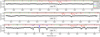 |
Fig. 1 Synthetic transmittance spectra for three diffraction orders measured by ACS MIR in the bottom of the detector frame in the secondary grating position 11. Contributions for water vapour, semi-heavy water vapour, and hydrogen chloride absorption are shown in blue, green, and red, respectively. Solar lines are shown in grey. The example of the measured spectra is shown in black in each diffraction order. The presented spectra are recorded during MY34 at Ls = 288° and latitude −54°S at 19 km tangent altitude. |
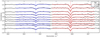 |
Fig. 2 Measured transmittances (black crosses) and the isotopologues absorption lines independent spectral fitting (blue and red curves) for ten detector rows. The vertical separation in the transmittance reflects the actual splits in altitudes and aerosol loadings sounded by different detector rows. All presented spectra are measured simultaneously within one frame. The corresponding tangent altitudes are from 19.1 to 20.6 km. These spectra are recorded at the same location as spectra from Fig. 1; the retrieved VMR of HCl is 1 ppb. |
4 Data processing
The calculation of transmittances as a function of tangent altitude is carried out in a standard manner for occultation experiments and as described previously for the case of ACS MIR (see also Trokhimovskiy et al. 2020; Korablev et al. 2019, SSM). We follow the robust calibration approach to treat each pixel of the detector array individually. In this work, we target very weak lines with depths approaching the noise level and face the problem of fixed pattern noise. To our understanding, the systematic features in the ACS MIR transmittance spectra originate mainly from what can be called the dark current non-linearity. To compensate for this, we use several tens of dark frames measured during a complete eclipse. These include the detector dark current and the thermal background. For every pixel, the observed values are linearly extrapolated over the whole occultation. However, as follows from dedicated calibration sessions, the linear approximation is not always perfectly followed. The remaining level of fixed pattern noise does not exceed 0.05% of the transmittance that still affects small lines. Additionally, the fixed pattern noise often exhibits a four-pixel pattern related to the four video outputs of the MIR channel, each served by its own ADC. Together, these two factors result in a fixed pattern noise along the altitudes and are non-repeating between orbits. This noise also has a vertical pattern in the spectra, for example repeating from row to row; this pattern is probably related to the FPA manufacturing (pixel size variations, e.g.). Consequently, the rows binning does not improve the confidence to measure small absorption lines. We thus decided to analyse detector rows independently without vertical averaging, further investigating all the retrievals from the nearby spectra.
Each of the diffraction orders 173–175 contains a doublet of HCl lines: one H35 Cl and one H37Cl (see Fig. 1). The two lines are close at the detector array, separated by only 50 pixels. This ensures that any possibleunaccounted optical effects are minimised. We also inspected the sensitivity to different calibration approaches, including stray light removal (Trokhimovskiy et al. 2020; Olsen et al. 2021a), and found no noticeable influence.
The three considered diffraction orders are of different value for the isotopologue study. Order 173 is located higher on the detector array where the solar signal is stronger, providing higher S/N; the advantage is overshadowed by weaker HCl lines. Furthermore, the H35 Cl line in this order lies close to a water vapour line, and the H2O retrieval becomes an additional source of uncertainty (Fig. 1). Order 175 also contains a water vapour line close to the HCl line. Moreover, the position of a solar line overlaps the weaker H37 Cl line. Ideally,solar lines should not affect the transmittance spectra, but even a slight mismatch in spacecraft pointing over the occultation causes a perturbation around the solar line. Above that, the HCl lines in order 175 are located lower and to the side at the detector, making the records noisier. Order 174 is optimal for the isotopologueanalysis: the HCl lines are strong, the lines and the surrounding baseline are clear from any contamination, with good S/N. Further results were obtained by examining data from order 174. The solar line right after 2927 cm−1 serves to fine-tune the pixel to wavenumber calibration of every spectrum.
Information about the atmospheric state for the retrieval was taken from simultaneous ACS near-infrared channel (NIR) measurements (Korablev et al. 2018a; Fedorova et al. 2020). The HCl isotopologue lines considered in this work have almost identical temperature dependences (Gordon et al. 2017), so even a small mismatch in temperature does not affect the isotopologue ratio. For example, with the increase in temperature from 180K to 240 K the H37 Cl line strength in order 174 increases by 27.07%, while the H35Cl line strength increases by nearly the same value of 27.05%. The uncertainties ranges for the lines intensities used in this study are listed in the HITRAN2016 database as 5–10% for H37 Cl and 1–2% for H35Cl.
The retrieval of H35Cl and H37Cl is done for spectra from every considered detector line by the iterative Levenberg-Marquardt iterative algorithm with Tikhonov regularisation developed to analyse SPICAM IR/MEx and ACS NIR data (Fedorova et al. 2018, 2020). For every spectral fit, we do eight iterations using the preceding solution as the initial assumption for the next run. The free parameters are aerosol extinction and the volume mixing ratios of HCl and HDO; weak lines are present in order 174 (see Fig. 1). The uncertainty on the retrieved quantities is given by the covariance matrix of the solution. Unlike some other works with ACS MIR data (Alday et al. 2019; Olsen et al. 2021a), the instrument line shape (ILS) is not fitted during the retrievals since in most cases the HCl lines too weak for that. The ILS was separately derived from the observations with the strongest HCl features and implemented into retrieval procedure as a fixed input. Furthermore, since the lines of interest are close on the detector and optically formed in a similar way, we consider these to have a similar ILS. Hydrogen chloride isotopologues are retrieved independently: H37 Cl in the range 2922.5–2924.6 cm−1 and H35Cl in the range 2924.8–2927.4 cm−1. The red and blue curves in Fig. 2 demonstrate the fit of the isotopologue absorption lines. Retrieval of the heavier isotopologue is done with the HITRAN convention with the SMOC ratio (0.32) already accounted for in the line strengths. The retrieved concentrations are in general agreement with the retrieval results in other works on HCl in the atmosphere of Mars (Olsen et al. 2021b; Aoki et al. 2021). A comparison with (Olsen et al. 2021b) is shown in Fig. 3. On average, we observe a shift towards smaller values obtained in this work. The most probable source of the difference is the ILS assumed in direct modelling. This detail does not affect the results since we derive the ratio of two oneness retrieved values.
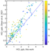 |
Fig. 3 Comparison of the retrieved HCl abundances in this work and in Olsen et al. (2021b). The colour bar stands for the tangent altitude in kilometres at which the measurements were performed. |
5 Results
Examples of the retrieval results of the H35Cl and H37Cl lines and their ratios from two selected orbits are shown in Fig. 4. Profiles retrieved from ten spectra corresponding to different detector rows are shown at their unique altitudes. The data are grouped by their corresponding row positions at each tangent height in the occultation sequence. The mean ratios for the ten detector rows are also shown in panels C and F. The H37 Cl retrievals have more variation because the spectral line is weaker than the H35 Cl line (see Fig. 1). The ratios of H37Cl and H35Cl are derived for each row. Since the retrievals were done with the assumed SMOC fractionation (embedded in HITRAN line strengths), the x-axis presents the fractionation factor against the terrestrial 0.32 value. We do not expect any variation on a vertical scale of a few kilometres from spectra within a single acquisition. Hence, the spread of the values from one frame (distinct colours in Fig. 4 for close tangent heights) reflects the factual errors of the measurements and retrievals. The average value of the ten ratio profiles obtained from one frame is shown in black diamonds with the standard deviation error bars. The vertical binning of the average is the same as the vertical sampling for a single row. At high altitudes, the lines are too weak to provide confident retrievals, while at low altitudes, the solar signal is too low because of the aerosol absorption. In both cases, uncertainties grow dramatically. Still, a portion of the profile at mid-heights demonstrates an optimal study case with the lowest uncertainty. For further analysis, we filter out points with errors bigger than 400‰ (0.4 in terms of comparing to SMOC).
For example, one of the best measurements in terms of precision provides a value of H37 Cl / H35 Cl = 0.98 ± 0.08 at 18 km altitude relative to SMOC, or δ37 Cl = −20 ± 80‰ in the per mil notation. This value from orbit 13 021 N2 presented in Fig. 4 was measured at the end of southern summer MY35 at Ls = 302° and latitude −65°S. Another southern orbit at Ls = 292° (19 sols earlier) demonstrates a very close value of the δ37 Cl = 6 ± 95‰ at 22 km. Within similar uncertainties, we found no time variation during southern summer in MY 34 and MY 35.
A number of orbits provide the possibility to check for variability over altitude. Orbit 4351 N1 shown in Fig. 4, allows us to retrieve values between altitudes of 23 km and 38 km with uncertainties of 110–210‰ around the mean value δ37 Cl = 40‰. This profile was obtained at MY34 at Ls = 288° and latitude −54°S. One of the best-confidence values at low altitude was retrieved during occultation 5030 N2 at 9.8 km and is δ37 Cl = 10 ± 120‰ at Ls = 320° in MY34 and latitude −71°S.
As mentioned earlier, hydrogen chloride abundances in the northern hemisphere are generally lower, making it hard to retrieve the isotopologue ratio with reasonable accuracy. The smallest uncertainty from a single observation was δ37 Cl = 120 ± 180‰, which was obtained in the northern winter at Ls = 260° in MY34 (orbit 3814 N1) at a latitude of 53°N.
With no apparent trend or variation found in our dataset within available altitudes, locations, and seasons, we can derive a weighted mean ratio from the ACS MIR measurements δ37 Cl = −7 ± 20‰ for the Martian atmospheric HCl isotopologues. This value comes from all selected 29 orbits; the mean is calculated from a collection of 77 ratios with an error less than 400‰. The values and their uncertainties are shown in Fig. 5.
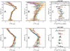 |
Fig. 4 Vertical profiles of H37Cl and H35 Cl isotopologues retrieved for two example orbits (Panel A, B, D, and E). The different colours represent retrievals done over spectra from ten different detector rows obtained from one frame. The corresponding profiles of the 37Cl/35Cl ratio in HCl are shown in Panels C and F. The average ratio profile is shown in black diamonds with the standard deviation error bars. |
6 Discussion
From the occultations measured with ACS MIR the HCl isotope ratio of 37Cl to 35Cl in the atmosphere of Mars is found to be close to the terrestrial value (SMOC). The atmospheric unit most probably reflects the initial distribution of chlorine on the planet. From the analysis of available Martian meteorites, we know that the Earth and Mars likely had a similar initial δ37 Cl at the time of theirformation. Analysis of Cl-bearing phosphate minerals from basalts in Martian meteorites without late-stage hydrothermal additions of halogens indicate these phosphate minerals have a Cl isotopic composition that is identical to the terrestrial mantle (Bellucci et al. 2017). The chlorine isotope composition of 16 Martian meteorites was also studied by Sharp et al. (2016). Measured δ37 Cl values range from −3.8 to 8.6‰. These authors proposed that relatively low δ37Cl values of −4‰ to −3‰ represent the primordial bulk composition of Mars inherited during accretion. Higher δ37 Cl values were found in all Martian samples that have evidence of crustal contamination. These moderate variations imply that the initial Cl isotopic composition for the Earth, Mars, and all inner solar system materials is identical or close within 10‰. High precision laboratory meteorite analyses fall within error bars of the value obtained in this work for atmospheric HCl isotopologues in the current epoch.
The chlorine ratio in the volcanic gases on Earth varies within a few per mils, reaching up to 10–20‰ in rare cases (Barnes et al. 2008, 2009; Rizzo et al. 2013). Thus our measurements of the HCl isotopologue ratio on Mars with an error bar of ~20‰ cannot be used to justify or deny the volcanic source of the HCl in the atmosphere.
Since the hydrogen chloride in the atmosphere of Mars has a clear seasonal pattern (Aoki et al. 2021; Olsen et al. 2021b), it is likely connected to a surface reservoir, such as NaCl bearing dust. Farley et al. (2016) report Cl isotope ratios measured by the SAM instrument on Curiosity from HCl thermally evolved from as-yet-unknown phases in sedimentary rocks and sand from Gale Crater. In this experiment, HCl is released during heating up to 600 °C, by a process very different from the atmospheric chemistry that is supposed to form the hydrogen chloride considered in this work. Seven samples yielded unexpectedly depleted and highly variable δ37 Cl values ranging from −1 ± 25‰ to −51 ± 5‰ and were attributed to oxidative perchlorate formation and reduction. Interpretation of the δ37 Cl results in Martian soils requires knowledge of the phase or phases from which Cl was extracted. At present, the source phase remains uncertain, but oxidation is the only mechanism that is able to generate large negative δ37 Cl anomalies (Sharp et al. 2007, 2013). Six of the samples from sedimentary rocks were obtained as cuttings from ~5 cm deep drill holes. The seventh, a sample of windblown sand, was acquired by scooping (Leshin et al. 2013). This is probably the most meaningful sample for comparing with volatiles ratios because it is from modern sand-drift deposits likely involved in the dust lifting process and active interaction with the atmosphere. Interestingly, although the sand sample has large uncertainty of 44‰, it has one of the highest values for the δ37 Cl of −7‰, which perfectly matches the mean value for the atmospheric HCl derived in this work. This supports the hypothesis that the lifted dust is involved in hydrogen chloride production on Mars.
Our hydrogen chloride measurements are mostly limited to an altitude range over which we have the greatest sensitivity from solar occultation geometry: 10–40 km. At higher altitudes we cannot provide ppb accuracy of the H37 Cl isotopologue measurements. Given this limitation, we could not find any sign of vertical dependence in the HCl fractionation. This first suggests that the fractionation effect (if any) is not as strong as for the Earth’s stratosphere chlorine components such as CF2Cl2. Laube et al. (2010) reported a positive fractionation up to 27‰ and probably more at higher altitudes due to preferential photolysis of the 35Cl isotopologue. The relative photolysis rates for the HCl chloride isotopologues are not well known, plus we are observing at low altitudes where aerosols already deplete UV radiation. The absence of vertical variation also implies that we cannot see any fast fractionation mechanism, for example owing to an H2O-HDO condensation rate difference (Montmessin et al. 2005). Typically for the season observed in this work, the hydrogen fractionation decreases over hygropause at 40 km (Villanueva et al. 2021). In the southern fall (Ls = 315°) the D/H ratio drops from 5 to 2 already above 20 km, where a large fraction of the HDO is sequestered. Our observations of hydrogen chloride isotopologues around Ls = 315° are limited just by 20 km altitude. This fact is connected to a striking similarity of HCl with the water vapour vertical distribution (Aoki et al. 2021). Above the 20 kilometres level water vapour starts to condense rapidly and the HCl abundance decreases as well, limiting us in chloride fractionation retrieval.
Another acknowledged source of isotopic fractionation for Mars atmospheric components is the escape as a consequence of lower gravity and solar wind interaction with the upper atmosphere (Jakosky et al. 1994). Lighter isotopes of argon have a similar mass to HCl and 38Ar/36Ar in the atmosphere of Mars was measured by the SAM instrument (Atreya et al. 2013). With good accuracy, it was shown that 36Ar is depleted by about 260‰ relative to primordial Ar. In this way, the argon isotope ratio is similar to massively fractionated water isotopologues D/H (Villanueva et al. 2015), while the HCl fractionation observed in this work is not even close to such large values. This leads us to the conclusion that the observed HCl and its chlorine isotopes have not participated in long-term atmospheric erosion.
High variability and rapid disappearance of the observed hydrogen chloride suggest that its lifetime in the atmosphere is short, maybe of an order of weeks or even less, an order of magnitude smaller than theoretical estimations of 90–1000 sol (Aoki et al. 2021). While dust and water vapour prevail in the atmosphere in southern summer, HCl can be observed at a certain orbit and be absent at the following one on the same day in similar latitudes. Such short timescales imply a particular pathway of HCl formation and its rapid deposition and/or adsorption at the surface or destruction in the atmosphere. We cannot check if the photodissociation or atmospheric escape plays a role in the enrichment during the HCl lifetime. No variation in the enrichment value with time can be noticed within our error bars. A gradual fractionation during photodissociation and lighter isotopologue atmospheric escape may occur with time in the overall chlorine cycle. But if even a fraction of the surface chlorine is involved in a multi-annual cycle with the atmosphere, these processes will cause an incremental chlorine fractionation chlorine fractionation in both reservoirs that is detectable in the atmosphere.There can still be a one-way path, where production and return to the ground are connected to different compounds.
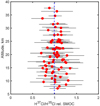 |
Fig. 5 Collection of 77 ratios and their errors of H37Cl over H35Cl, each obtained from 10 spectra within a single diffraction order stripe, with an error less than 400‰ measured on 29 orbits in total. The weighted mean value is δ37 Cl = −7 ± 20‰ for the Martian atmospheric HCl isotopologues is plotted with a vertical blue dashed line. |
7 Conclusions
The discovery of the hydrogen chloride gas in the atmosphere of Mars makes it another marker of surface-atmosphere interaction processes and chemistry. With sporadic exceptions HCl is observed in both hemispheres during southern summer, with maximum values of ~5 ppb at southern latitudes. In contrast to other volatile species on Mars, HCl does not demonstrate fractionation in the atmosphere compared to the terrestrial values. On average, the δ37Cl was found to be − 7 ± 20‰; a small depletion still covers SMOC within uncertainties. This result is consistent with known meteorites and Martian soil properties, supporting the idea of HCl formation from chlorine bearing dust grains.
Within the accuracy of the retrieved values from ACS MIR measurements, we are not able to detect any δ37 Cl variation in time or over the planet. That leads us to conclude that all suggested fractionating mechanisms are too weak to be noticed in the atmospheric hydrogen chloride isotopologues, especially considering the short lifetime of HCl. It is also unlikely that the chlorine isotopes we observe in HCl are involved in any long-term chlorine cycle between the soil and the atmosphere.
Acknowledgements
ExoMars is a joint space mission of the European Space Agency (ESA) and Roscosmos. The ACS experiment is led by the Space Research Institute (IKI) in Moscow, assisted by LATMOS in France. Data processing and analysis for this study in IKI are funded by subsidy of the Ministry of High Education and Science. Work at the University of Oxford was funded by the UK Space Agency (ST/T002069/1, ST/R001502/1).
References
- Alday, J., Wilson, C. F., Irwin, P. G. J., et al. 2019, A&A, 630, A91 [CrossRef] [EDP Sciences] [Google Scholar]
- Alday, J., Trokhimovskiy, A., Irwin, P. G., et al. 2021, Nat. Astron., accepted [Google Scholar]
- Aoki, S., Daerden, F., Viscardy, S., et al. 2021, Geophys. Res. Lett., accepted [Google Scholar]
- Atreya, S. K., Trainer, M. G., Franz, H. B., et al. 2013, Geophys. Res. Lett., 40, 5605 [CrossRef] [Google Scholar]
- Barnes, J. D., Sharp, Z. D., & Fischer, T. P. 2008, Geology, 36, 883 [CrossRef] [Google Scholar]
- Barnes, J. D., Sharp, Z. D., Fischer, T. P., Hilton, D. R., & Carr, M. J. 2009, Geochem. Geophys. Geosyst., 10, 11 [CrossRef] [Google Scholar]
- Bellucci, J. J., Whitehouse, M. J., John, T., et al. 2017, Earth Planet. Sci. Lett., 458, 192 [CrossRef] [Google Scholar]
- Berger, J. A., Schmidt, M. E., Gellert, R., et al. 2016, Geophys. Res. Lett., 43, 67 [CrossRef] [Google Scholar]
- Berglund, M., & Wieser, M. E. 2011, Pure Appl. Chem., 83, 397 [CrossRef] [Google Scholar]
- Böhlke, J. K., Sturchio, N. C., Gu, B., et al. 2005, Anal. Chem., 77, 7838 [CrossRef] [Google Scholar]
- Bogard, D. D., Clayton, R. N., Marti, K., Owen, T., & Turner, G. 2001, Space Sci. Rev., 96, 425 [CrossRef] [Google Scholar]
- Bonifacie, M. 2018, Chlorine Isotopes, ed. W. M. White (Cham: Springer International Publishing), 244 [Google Scholar]
- Catling, D. C., Claire, M. W., Zahnle, K. J., et al. 2010, J. Geophys. Res., 115, E00E11 [Google Scholar]
- Cheng, B.-M., Chew, E. P., Liu, C.-P., et al. 1999, Geophys. Res. Lett., 26, 3657 [NASA ADS] [CrossRef] [PubMed] [Google Scholar]
- Clark, B. C., & Kounaves, S. P. 2016, Int. J. Astrobiol., 15, 311 [Google Scholar]
- Encrenaz, T., Greathouse, T. K., Richter, M. J., et al. 2011, A&A, 530, A37 [NASA ADS] [CrossRef] [EDP Sciences] [Google Scholar]
- Encrenaz, T., DeWitt, C., Richter, M. J., et al. 2018, A&A, 612, A112 [CrossRef] [EDP Sciences] [Google Scholar]
- Farley, K. A., Martin, P., Archer, P. D., et al. 2016, Earth Planet. Sci. Lett., 438, 14 [CrossRef] [Google Scholar]
- Fedorova, A., Bertaux, J.-L., Betsis, D., et al. 2018, Icarus, 300, 440 [NASA ADS] [CrossRef] [Google Scholar]
- Fedorova, A. A., Montmessin, F., Korablev, O., et al. 2020, Science, 367, 297 [CrossRef] [Google Scholar]
- Fedorova, A., Montmessin, F., Korablev, O., et al. 2021, J. Geophys. Res. Planets, 126, e06616 [CrossRef] [Google Scholar]
- Glavin, D. P., Freissinet, C., Miller, K. E., et al. 2013, J. Geophys. Res., 118, 1955 [Google Scholar]
- Godon, A., Jendrzejewski, N., Eggenkamp, H. G. M., et al. 2004, Chem. Geol., 207, 1 [CrossRef] [Google Scholar]
- Gordon, I. E., Rothman, L. S., Hill, C., et al. 2017, J. Quant. Spectr. Rad. Transf., 203, 3 [Google Scholar]
- Hecht, M. H., Kounaves, S. P., Quinn, R. C., et al. 2009, Science, 325, 64 [Google Scholar]
- Hu, R. 2019, LPI Contrib., 2089, 6255 [Google Scholar]
- Jackson, W. A., Böhlke, J. K., Andraski, B. J., et al. 2015, Geochim. Cosmochim. Acta, 164, 502 [CrossRef] [Google Scholar]
- Jakosky, B. M., & Phillips, R. J. 2001, Nature, 412, 237 [NASA ADS] [CrossRef] [Google Scholar]
- Jakosky, B. M., Pepin, R. O., Johnson, R. E., & Fox, J. L. 1994, Icarus, 111, 271 [CrossRef] [Google Scholar]
- Kaufmann, R., Long, A., Bentley, H., & Davis, S. 1984, Nature, 309, 338 [CrossRef] [Google Scholar]
- Keller, J. M., Boynton, W. V., Karunatillake, S., et al. 2006, J. Geophys. Res., 111, E03S08 [Google Scholar]
- Khayat, A. S., Villanueva, G. L., Mumma, M. J., & Tokunaga, A. T. 2015, Icarus, 253, 130 [CrossRef] [Google Scholar]
- Korablev, O., Montmessin, F., Trokhimovskiy, A., et al. 2018a, Space Sci. Rev., 214, 7 [NASA ADS] [CrossRef] [Google Scholar]
- Korablev, O. I., Belyaev, D. A., Dobrolenskiy, Y. S., Trokhimovskiy, A. Y., & Kalinnikov, Y. K. 2018b, Appl. Opt., 57, C103 [CrossRef] [Google Scholar]
- Korablev, O., Vandaele, A. C., Montmessin, F., et al. 2019, Nature, 568, 517 [CrossRef] [Google Scholar]
- Korablev, O., Olsen, K. S., Trokhimovskiy, A. et al. 2021, Sci. Adv., 7, eabe4386 [Google Scholar]
- Krasnopolsky, V. A. 2012, Icarus, 217, 144 [NASA ADS] [CrossRef] [Google Scholar]
- Krasnopolsky, V. A. 2015, Icarus, 257, 377 [NASA ADS] [CrossRef] [Google Scholar]
- Krasnopolsky, V. A. 2021, Icarus, submitted [Google Scholar]
- Laube, J. C., Kaiser, J., Sturges, W. T., Bönisch, H., & Engel, A. 2010, Science, 329, 1167 [CrossRef] [Google Scholar]
- Lee, J.-Y., Marti, K., Severinghaus, J. P., et al. 2006, Geochim. Cosmochim. Acta, 70, 4507 [CrossRef] [Google Scholar]
- Lefèvre, F., Lebonnois, S., Montmessin, F., & Forget, F. 2004, J. Geophys. Res., 109, E07004 [Google Scholar]
- Leshin, L. A., Mahaffy, P. R., Webster, C. R., et al. 2013, Science, 341, 1238937 [CrossRef] [Google Scholar]
- Mahieux, A., Wilquet, V., Vandaele, A. C., et al. 2015, Planet. Space Sci., 113, 264 [CrossRef] [Google Scholar]
- Montabone, L., Spiga, A., Kass, D. M., et al. 2020, J. Geophys. Res., 125, e06111 [Google Scholar]
- Montmessin, F., Fouchet, T., & Forget, F. 2005, J. Geophys. Res., 110, E03006 [NASA ADS] [CrossRef] [Google Scholar]
- Ohno, M., Utsugi, M., Mori, T., et al. 2013, Earth Planets Space, 65, e1 [CrossRef] [Google Scholar]
- Olsen, K. S., Lefèvre, F., Montmessin, F., et al. 2020, A&A, 639, A141 [CrossRef] [EDP Sciences] [Google Scholar]
- Olsen, K. S., Lefèvre, F., Montmessin, F., et al. 2021a, Nat. Geosci., 14, 67 [CrossRef] [Google Scholar]
- Olsen, K. S., Trokhimovskiy, A., Montabone, L., et al. 2021b, A&A, 647, A161 [NASA ADS] [CrossRef] [EDP Sciences] [Google Scholar]
- Owen, T., Maillard, J. P., de Bergh, C., & Lutz, B. L. 1988, Science, 240, 1767 [NASA ADS] [CrossRef] [PubMed] [Google Scholar]
- Potts, N. J., Barnes, J. J., Tartèse, R., Franchi, I. A., & Anand, M. 2018, Geochim. Cosmochim. Acta, 230, 46 [Google Scholar]
- Rizzo, A. L., Caracausi, A., Liotta, M., et al. 2013, Earth Planet. Sci. Lett., 371, 134 [Google Scholar]
- Sharp, Z. D., Barnes, J. D., Brearley, A. J., et al. 2007, Nature, 446, 1062 [Google Scholar]
- Sharp, Z. D., Shearer, C. K., McKeegan, K. D., Barnes, J. D., & Wang, Y. Q. 2010, Science, 329, 1050 [Google Scholar]
- Sharp, Z. D., McCubbin, F. M., & Shearer, C. K. 2013, Earth Planet. Sci. Lett., 380, 88 [Google Scholar]
- Sharp, Z., Williams, J., Shearer, C., Agee, C., & McKeegan, K. 2016, Meteorit. Planet. Sci., 51, 2111 [Google Scholar]
- Smith, M. L., Claire, M. W., Catling, D. C., & Zahnle, K. J. 2014, Icarus, 231, 51 [NASA ADS] [CrossRef] [Google Scholar]
- Sturchio, N. C., Böhlke, J. K., Gu, B., et al. 2006, Stable Isotopic Composition of Chlorine and Oxygen in Synthetic and Natural Perchlorate, eds. B. Gu, & J. D. Coates (Boston, MA: Springer US), 93 [Google Scholar]
- Sturchio, N. C., Böhlke, J. K., Gu, B., Hatzinger, P. B., & Jackson, W. A. 2012, Isotopic Tracing of Perchlorate in the Environment, ed. M. Baskaran (Berlin, Heidelberg: Springer Berlin Heidelberg), 437 [Google Scholar]
- TartèSe, R., Anand, M., Joy, K. H., & Franchi, I. A. 2014, Meteorit. Planet. Sci., 49, 2266 [Google Scholar]
- Trokhimovskiy, A., Fedorova, A., Korablev, O., et al. 2015, Icarus, 251, 50 [NASA ADS] [CrossRef] [Google Scholar]
- Trokhimovskiy, A., Perevalov, V., Korablev, O., et al. 2020, A&A, 639, A142 [EDP Sciences] [Google Scholar]
- Vago, J., Witasse, O., Svedhem, H., et al. 2015, Sol. Syst. Res., 49, 518 [CrossRef] [Google Scholar]
- Vandaele, A. C., Korablev, O., Daerden, F., et al. 2019, Nature, 568, 521 [NASA ADS] [CrossRef] [Google Scholar]
- Villanueva, G. L., Mumma, M. J., Novak, R. E., et al. 2015, Science, 348, 218 [NASA ADS] [CrossRef] [Google Scholar]
- Villanueva, G. L., Liuzzi, G., Crismani, M. M. J., et al. 2021, Sci. Adv., 7 [Google Scholar]
- Webster, C. R., Mahaffy, P. R., Atreya, S. K., et al. 2013, Science, 342, 355 [NASA ADS] [CrossRef] [Google Scholar]
- Wilson, E. H., Atreya, S. K., Kaiser, R. I., & Mahaffy, P. R. 2016, J. Geophys. Res., 121, 1472 [NASA ADS] [CrossRef] [Google Scholar]
- Wong, M. H., Atreya, S. K., Mahaffy, P. N., et al. 2013, Geophys. Res. Lett., 40, 6033 [Google Scholar]
All Figures
|
Fig. 1 Synthetic transmittance spectra for three diffraction orders measured by ACS MIR in the bottom of the detector frame in the secondary grating position 11. Contributions for water vapour, semi-heavy water vapour, and hydrogen chloride absorption are shown in blue, green, and red, respectively. Solar lines are shown in grey. The example of the measured spectra is shown in black in each diffraction order. The presented spectra are recorded during MY34 at Ls = 288° and latitude −54°S at 19 km tangent altitude. |
| In the text | |
|
Fig. 2 Measured transmittances (black crosses) and the isotopologues absorption lines independent spectral fitting (blue and red curves) for ten detector rows. The vertical separation in the transmittance reflects the actual splits in altitudes and aerosol loadings sounded by different detector rows. All presented spectra are measured simultaneously within one frame. The corresponding tangent altitudes are from 19.1 to 20.6 km. These spectra are recorded at the same location as spectra from Fig. 1; the retrieved VMR of HCl is 1 ppb. |
| In the text | |
|
Fig. 3 Comparison of the retrieved HCl abundances in this work and in Olsen et al. (2021b). The colour bar stands for the tangent altitude in kilometres at which the measurements were performed. |
| In the text | |
|
Fig. 4 Vertical profiles of H37Cl and H35 Cl isotopologues retrieved for two example orbits (Panel A, B, D, and E). The different colours represent retrievals done over spectra from ten different detector rows obtained from one frame. The corresponding profiles of the 37Cl/35Cl ratio in HCl are shown in Panels C and F. The average ratio profile is shown in black diamonds with the standard deviation error bars. |
| In the text | |
|
Fig. 5 Collection of 77 ratios and their errors of H37Cl over H35Cl, each obtained from 10 spectra within a single diffraction order stripe, with an error less than 400‰ measured on 29 orbits in total. The weighted mean value is δ37 Cl = −7 ± 20‰ for the Martian atmospheric HCl isotopologues is plotted with a vertical blue dashed line. |
| In the text | |
Current usage metrics show cumulative count of Article Views (full-text article views including HTML views, PDF and ePub downloads, according to the available data) and Abstracts Views on Vision4Press platform.
Data correspond to usage on the plateform after 2015. The current usage metrics is available 48-96 hours after online publication and is updated daily on week days.
Initial download of the metrics may take a while.