| Issue |
A&A
Volume 649, May 2021
|
|
|---|---|---|
| Article Number | A111 | |
| Number of page(s) | 9 | |
| Section | Planets and planetary systems | |
| DOI | https://doi.org/10.1051/0004-6361/202040201 | |
| Published online | 24 May 2021 | |
Stellar clustering and orbital architecture of planetary systems★
1
Instituto de Astrofísica e Ciências do Espaço, Universidade do Porto, CAUP,
Rua das Estrelas,
4150-762 Porto, Portugal
e-mail: This email address is being protected from spambots. You need JavaScript enabled to view it.
2
Departamento de Física e Astronomia, Faculdade de Ciências, Universidade do Porto, Rua do Campo Alegre,
4169-007
Porto, Portugal
3
European Southern Observatory,
Alonso de Córdova 3107,
Vitacura,
Región Metropolitana, Chile
4
Instituto de Astrofísica de Canarias,
38205
La Laguna,
Tenerife, Spain
5
Departamento de Astrofìsica, Universidad de La Laguna,
38206
La Laguna,
Tenerife, Spain
6
Center for Cosmology and Astrophysics, Alikhanian National Science Laboratory,
2 Alikhanian Brothers Str.,
0036
Yerevan, Armenia
Received:
22
December
2020
Accepted:
26
February
2021
Abstract
Context. Revealing the mechanisms shaping the architecture of planetary systems is crucial for our understanding of their formation and evolution. In this context, it has been recently proposed that stellar clustering might be the key in shaping the orbital architecture of exoplanets.
Aims. The main goal of this work is to explore the factors that shape the orbits of planets.
Methods. We performed different statistical tests to compare the properties of planets and their host stars associated with different stellar environments.
Results. We used a homogeneous sample of relatively young FGK dwarf stars with radial velocity detected planets and tested the hypothesis that their association to phase space (position-velocity) over-densities (“cluster” stars) and under-densities (“field” stars) impacts the orbital periods of planets. When controlling for the host star properties on a sample of 52 planets orbiting around cluster stars and 15 planets orbiting around field stars, we found no significant difference in the period distribution of planets orbiting these two populations of stars. By considering an extended sample of 73 planets orbiting around cluster stars and 25 planets orbiting field stars, a significant difference in the planetary period distributions emerged. However, the hosts associated with stellar under-densities appeared to be significantly older than their cluster counterparts. This does not allow us to conclude as to whether the planetary architecture is related to age, environment, or both. We further studied a sample of planets orbiting cluster stars to study the mechanism responsible for the shaping of orbits of planets in similar environments. We could not identify a parameter that can unambiguously be responsible for the orbital architecture of massive planets, perhaps, indicating the complexity of the issue.
Conclusions. An increased number of planets in clusters and in over-density environments will help to build large and unbiased samples which will then allow to better understand the dominant processes shaping the orbits of planets.
Key words: methods: statistical / planets and satellites: formation / planet-star interactions / stars: fundamental parameters
The ages of all the stars are only available at the CDS via anonymous ftp to cdsarc.u-strasbg.fr (130.79.128.5) or via http://cdsarc.u-strasbg.fr/viz-bin/cat/J/A+A/649/A111
© ESO 2021
1 Introduction
Understanding the mechanisms shaping the architecture of planetary systems is crucial to complete the picture of planet formation and evolution (e.g., Winn & Fabrycky 2015; Hatzes 2016). Among the many open questions in this field, it is of particular interest to understand the origin of hot Jupiters (HJs, Dawson & Johnson 2018) – short period giant planets1. Several mechanisms are proposed to explain the presence of these massive planets at very close distances to their host stars: in situ formation, disk migration, high-eccentricity tidal migration, and dynamical perturbations by stellar fly-bys in open clusters. Although, a combination of these mechanisms might be needed to explain the observational properties of HJs and their hosts stars (Dawson & Johnson 2018), it was suggested very recently that the short periods of HJs originate from environmental perturbations (Winter et al. 2020, hereafter, W20).
To study the possible link between stellar clustering and the architecture of planetary systems, Winter et al. (2020) estimated the probability (Phigh) that a planet host star belongs to over- or under-densities in the position-velocity phase space. The authors determined and made publicly available the Phigh values for more than 1500 exoplanet host stars for which radial velocities were available in Gaia Data Release 2 (DR2). Stars with Phigh > 0.84 were considered as potential members of co-moving groups (over-density or cluster stars) and stars with Phigh < 0.16 as field stars. Based on this database, they reached two important conclusions: Planets orbiting stars associated with over-densities have significantly shorter orbital periods than those orbiting around field stars and that HJs predominantly exist around cluster stars.
Given the importance of these findings and conclusions, in this manuscript we performed an independent analysis of their data but using homogeneously determined stellar parameters of the planet host stars from the SWEET-Cat (a catalogue of parameters for Stars With ExoplanETs; Santos et al. 2013). The manuscript is organized as follows: In Sect. 2, a homogeneous sample trying to control different biases is built and then, in Sect. 3 the period distribution of planets orbiting cluster and field stars is studied. In Sect. 4 we study the impact of different physical parameters on the orbital periods of the planets associated with high-density stellar environments. We summarize our work in Sect. 5.
2 SWEET-Cat FGK dwarf RV sample
In order to confirm or refute the main findings of Winter et al. (2020), it is crucial to perform the analysis on an unbiased sample. For a discussion about the impact of different (potential) biases, we refer the reader to W20. In this section we build a sample (based on the original full sample of W20) of radial velocity (RV) detected2 high-mass planets orbiting around FGK dwarf stars for which homogeneously derived (see Appendix A) stellar parameters exist in SWEET-Cat. We then perform a statistical analysis on this data using the Anderson–Darling (AD)3 test to study the impact of stellar clustering on the orbital periods of exoplanets. It is important to note that by restricting the sample to RV detected planets, we did not remove the observational biases from which this planet detection method suffers. However, wetry to minimize the impacts of different biases by applying further restrictions on the properties of planets and their hosts. Ideally, one would have to carefully model and correct for the detection biases to construct the actual period distributions of the planets. However, this would be extremely difficult since the planets of our sample come from different planet search programs that were all carried out with different instruments, observational strategies, and detection biases.
In this analysis we focus only on massive planets with masses between 50 M⊕ and 4 Mjup. The selected lower limit is the same as the one adopted in W20 for HJs. This semi-arbitrary limit (see the discussion in Adibekyan 2019) is considered to decrease the impact of planet detection limits (low-mass planets are difficult to detect in wide orbits) and also the planet core-accretion models predicted a minimum in the planetary mass-distribution at about 50 M⊕ mass (e.g., Mordasini et al. 2009). Our choice for the upper mass limit is motivated by the recent findings that the properties of stars hosting super-massive Jupiters (Mpl > 4 Mjup) are different from those hosting lower-mass Jupiters which might suggest different formation mechanisms (e.g., Santos et al. 2017; Adibekyan 2019; Maldonado et al. 2019; Goda & Matsuo 2019). The range of effective temperature of the selected FGK stars is 4500 < Teff < 6500 K. This is the range of temperatures for which SWEET-Cat provides most precise stellar parameters (e.g., Sousa et al. 2008). From our sample, we excluded the evolved stars (logg < 4.0 dex) because their properties (for example their mass and metallicity) and the properties of their planets (for example the orbital periods) show different distributions when compared with the properties of planets orbiting around dwarfs (e.g., Adibekyan et al. 2013; Maldonado et al. 2013; Mortier et al. 2013).
The aforementioned constraints led us to a sample of 178 FGK dwarf stars hosting 214 RV detected giant planets4. For all these stars, we homogeneously determined the isochrone ages using the PARAM (PARAM) v1.3 web interface5. The details of the age determination and the results of their comparison with the ages used in W20 are presented in Appendix B. We then applied the final cut on age as suggested in W20 (stars with ages between 1 and 4.5 Gyr) to build our main sample, hereafter called the FGKPlow,high sample. This sample consists of 44 Phigh6 (52 planets)and 14 Plow (15 planets) stars. The distribution of these planets on the period-mass diagram is shown in the left panel of Fig. 1.
3 Orbital periods of planets orbiting around Plow and Phigh stars
In Fig. C.1 we compare the cumulative distribution functions (CDFs) of different properties of planets and their host stars associated with over- and under-densities. The figure and the corresponding PAD values suggest that the planets orbiting these two groups of stars do not have significantly different distributions of the orbital periods. The figure also shows that the host star shows significantly different distributions of Teff and ages, the Phigh stars being hotter and younger than their Plow counterparts. In particular, only three out of the 15 planets orbiting Plow stars are younger than 3 Gyr. The number of planets (age < 3 Gyr) orbiting young Phigh stars is 32, which is about 60% (32 out of 52) of the whole sample.
Although in the aforementioned analysis the AD test does not reject the null hypothesis that, overall, distributions of periods of planets orbiting Phigh and Plow stars come from the same parent distribution, Fig. 1 visually suggests an overabundance of short period planets (periods shorter than about 10 to 30 days) around Phigh stars when compared to their Plow counterparts.The fraction of short period (period < 30 days7) planets orbiting Phigh stars is 23.1 % (12 out of 52). This number, being slightly larger, however, statistically speaking is not different from the one for the Plow sample: 20.0
 % (3 out of 15). The difference does not remain significant if one considers a more commonly used period limit of 10 days for HJs (e.g., Wang et al. 2015): 17.3
 % (nine out of 52) and 20.0
 % (three out of 15) for the HJs orbiting around Phigh and Plow stars, respectively.
Unfortunately, by applying the cut on age and selecting only RV detected planets, we significantly reduced the size of the sample, especially the number of Plow stars. The reduced sample size has a direct impact on the errors of the estimated HJ fractions and might be responsible for the insignificance of the aforementioned differences. Below, we try to expand the sample by increasing the range in stellar ages and relaxing the Phigh threshold.
In Fig. 2 we show the fraction of HJs orbiting stars associated with over- and under-densities as a function of the Phigh threshold, which is used to separate the stars into these two categories. In the figure, we considered 10, 20, and 30 days as the upper limit for the orbital periods of HJs. The figure shows that the maximum difference of the fraction of HJs orbiting around cluster and field stars is observed at the Phigh threshold of 0.3. This difference is, however, notsignificant at even one-σ level. The figure also shows that, as for the main sample, the two groups of stars have a significantly different distribution of ages. In the following, for the tests, we adopt the 0.3 value as the Phigh threshold, which allows one to both increase the sample size and decrease the contamination of the samples by excluding the stars with intermediate Phigh probabilities.
To further increase the sample size, we reduced the lower age limit from 1 to 0.5 Gyr. Although individual planets or planetary systems can show instabilities at timescales of a few gigayears (in fact, one of the phenomena responsible for the instability on long timescales is the fly-by encounters that can occur in dense stellar environments, Davies et al. 2014), usually the orbits of massive planets become stable at less than about 100 Myr (e.g., Raymond et al. 2009; Davies et al. 2014; Sotiriadis et al. 2017; Bitsch et al. 2020). As discussed in W20 (also see Kruijssen et al. 2020), going beyond 5 Gyr leads to a strong contamination of the field sample by former over-density stars and should be avoided. In general, the younger the stars are, the easier and more reliable their association to over- or under-density stellar environments.
Figure 3 shows the fraction of HJs orbiting stars associated to over- and under-densities as a function of the upper limit of stellar ages. The figure shows that the HJ fractions are statistically speaking similar up to an upper age limit of 5 Gyr. Moreover, the difference in the HJ fraction with age increases mostly because of the decrease in the fraction of HJs orbiting field stars. This is somehow counterintuitive, because as it was mentioned earlier, older field samples are more contaminated by former cluster stars for which the fraction of HJs becomes higher. Up to ages of 3 Gyr, the fraction of HJs orbiting around field stars is even higher than that for the cluster stars. However, it is important to note that the number of Plow stars with ages below 3 Gyris very small. Figure 3 also shows that when going beyond the 5 Gyr limit, the HJ fraction slightly decreases for both Plow and Phigh samples. This is because on average the hosts of HJs are slightly younger than the hosts of their longer period counterparts. This result is similar to the one of Hamer & Schlaufman (2019) where the authors concluded that tidal interactions cause HJs to inspiral on a timescale shorter than the main sequence lifetime of the stars.
Considering stars with ages between 0.5 and 5 Gyr as well as the Phigh threshold of 0.3, we constructed an extended sample consisting of 73 planets orbiting Phigh stars and 25 planets orbiting Plow stars. The distributions of these planets in the period-mass diagram is shown in the right panel of Fig. 1. The difference in the HJ fractions between the two groups is largest when considering an upper orbital period limit of 30 days for HJs. This difference (28.8 % (21 out of 73) and 12.0
 % (3 out of 25) is significant at about the 80% level, which would correspond to ~1.3σ for a Gaussian distribution. However, it is important to stress again the statistically significant difference in age as inferred from the p-values of the AD test (see Fig. C.2).
For the extended sample, Fig. C.2 suggests a statistically significant difference for the period distributions of planets orbiting stars in over- and under-densities. However, the two subsamples show statistically different distributions in planetary mass, Teff, and stellar age. Restricting the sample (25 and 22 planets orbiting around Phigh and Plow stars, respectively) to stars with ages between 2.5 and 5 Gyr and to planets with masses >150 M⊕ allows the differences in planetary mass, Teff, and stellar age to vanish. This restriction also dilutes the difference in the orbital period distributions (see Fig. C.3).
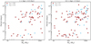 |
Fig. 1 Distribution of the RV detected planets on the period-mass diagram orbiting around FGK dwarf stars with homogeneously derived stellar parameters in SWEET-Cat. The left panel is for the FGKPlow,high sample and the right panel is for the planets in the expended sample. |
4 Properties of stars hosting short- versus long-period planets in over- and under-density environments
The analysis of the previous section did not reveal an unambiguous relation between stellar clustering and orbital architecture of exoplanets. In this section, we separate the Phigh and Plow samples to study the impact of the physical properties of the host stars on the orbital properties of giant planets. In this way, we eliminate the impact (if any) of stellar clustering on the architecture of planets.
Adibekyan et al. (2013) show that most of the massive planets orbiting low-metallicity stars ([Fe/H] < −0.1 dex) have orbital periods longer than about 100 days (see also Sozzetti 2004; Maldonado et al. 2012). The authors suggest that planets in a metal-poor disk are forming further out and/or undergoing less migration as they take longer to form. Recently, Osborn & Bayliss (2020) studied the metallicity distribution of HJs and found that although they preferentially orbit metal-rich stars, the average metallicity of their hosts is not higher than that of stars hosting cold Jupiters. The authors concluded that hot and cold Jupiters are formed in a similar process, but they have different migration histories. In complement to these results, Dawson & Murray-Clay (2013) and Buchhave et al. (2018) show that giant planets orbiting metal-rich stars show signatures of dynamical interaction. Buchhave et al. (2018), in particular, show that HJs and cold eccentric Jupiters are preferentially orbiting metal-rich stars, while cold Jupiters with circular orbits are mostly observed around solar-metallicity stars.
In the left and right panels of Fig. 4, we separately show the distribution of planets orbiting the Phigh and Plow stars of the extended FGKPlow,high sample. Due to the age constraints (young stars are on average metallic), the number of planets orbiting metal-poor stars (Fe/H] < 0.0 dex) in this sample is very small. However, as was found in Adibekyan et al. (2013), they all have orbital periods longer than 100 days.
Because the sample of Plow stars is very small, we focus only on the planets orbiting Phigh stars next. This sample consists of 21 planets with periods shorter than 30 days and 52 planets with longer periods. Figure C.4 shows the CDFs of these short- and long-periods planets and their host stars. As indicated by the PAD values, the two groups are significantly different only in the distribution of the planetary masses, the HJs having on average lower-masses. If the upper period limit is reduced to 10 or 20 days, the results remain practically the same. The fact that the age distribution of the short and long period planets are similar might indicate that tidal inspiral is not significantly depleting the short period planets in this age range. However, a dedicated analysis on a larger sample is required to draw a firm conclusion.
Unfortunately, out analysis does not allow us to firmly conclude which parameter(s) internal for the star–planet system is(are) responsible for the period distribution of exoplanets orbiting stars that formed in a similar stellar environment. This is perhaps due to the small size of the sample and/or due to the complexity of the problem.
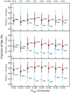 |
Fig. 2 Fraction of HJs orbiting cluster (brown) and field (skyblue) stars as a function of Phigh threshold which is used to separate the aforementioned two groups. The numbers next to the HJs fraction correspond to the numbers of HJs and the total number of planets that are used to compute these fractions. The upperlimit for the HJs orbital period was set at 10 (top), 20 (middle), and 30 (bottom) days. The PAD values on top of the panels show the results of the AD test comparing the distributions of the ages of the cluster and field stars. The errorbars represent a 68.3% (1σ) interval. |
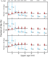 |
Fig. 3 Fraction of HJs orbiting cluster (brown) and field (skyblue) stars as a function of upper age limit. The lower age limit is set to 0.5 Gyr and the Phigh threshold was set to 0.3. The symbols and numbers are the same as in Fig. 2. |
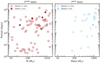 |
Fig. 4 Period-mass diagram of planets around FGK Phigh (left panel) and Plow (right panel) dwarf stars with homogeneously derived stellar parameters in SWEET-Cat. Only stars with ages between 1 and 4.5 Gyr are shown. Planets orbiting metal-poor and metal-rich stars are shown in open and filled circles, respectively. |
5 Summary and conclusion
Very recently, Winter et al. (2020) carried out tremendous work by assigning a large sample of exoplanet host stars to low- (Plow) or high-density(Phigh) stellar environments. The authors then used this sample to conclude that planets orbiting stars in high-density environments have significantly shorter periods and a smaller semi-major axis than their counterparts orbiting field (low-density) stars. They also found that most of the hot Jupiters are orbiting around cluster stars. These findings, if confirmed, may have very important implicationsfor our understanding of planet formation and evolution.
In this manuscript, we constructed a sample of FGK dwarf stars with only RV detected HJs for which homogeneously determined stellar parameters are available in the SWEET-Cat catalog (Santos et al. 2013). Additionally, we made further constraints on the upper mass of planets at 4 Mjup since the origin of the super-massive planets might be different (e.g., Santos et al. 2017; Adibekyan 2019). For this sample of stars, we homogeneously determined isochrone ages.
In this small but significantly less biased sample of stars with ages between 1 and 4.5 Gyr (52 planets orbiting Phigh stars and 15 planets orbiting Plow stars), we found no significant difference in the period distribution of planets orbiting Phigh and Plow stars. We then constructed an extended sample by slightly relaxing the constrains on age and the Phigh threshold. In this sample consisting of 73 planets orbiting around cluster stars and 25 planets orbiting around filed stars, we found a statistically significant difference for the period distributions of planets orbiting around these two populations of stars. However, the field and cluster stars also showed a significant difference in the stellar age. When controlling for the host star properties, the differences in orbital periods of planets orbiting around stars associated with the over- and under-densities diminish. Thus, it is not possible to conclude whether the planetary architecture is related to age, environment, or both.
Next we focused only on a subsample of planets orbiting Phigh stars with the aim of understanding the mechanism responsible for shaping their planetary orbits in similar environments. We could not identify a parameter that unambiguously can be responsible for the orbital architecture of these planets.
It is important to note that although our analysis does not suggest that the stellar clustering is the key parameter shaping the orbits of planets, it still can play a role, especially given some observational (e.g., Brucalassi et al. 2016) and theoretical (e.g., Shara et al. 2016; Vincke & Pfalzner 2018; Wang et al. 2020) support of this hypothesis. The full picture of planet survival in dense stellar environments is not simple and depends on many external and internal factors to star-planets (e.g., Stock et al. 2020, and references therein). An increased number of planet hosts in clusters and in over-density environments will help to build large and unbiased samples which will then shed light on this issue.
Acknowledgements
We thank the anonymous referee for the very constructive comments and suggestions which helped us to substantially improve the quality of the work amd presentations of the results. This work was supported by FCT – Fundação para a Ciência e Tecnologia (FCT) through national funds and by FEDER through COMPETE2020 – Programa Operacional Competitividade e Internacionalização by these grants: UID/FIS/04434/2019; UIDB/04434/2020; UIDP/04434/2020; PTDC/FIS-AST/32113/2017 and POCI-01-0145-FEDER-032113; PTDC/FIS-AST/28953/2017 and POCI-01-0145-FEDER-028953. V.A., E.D.M, N.C.S., and S.G.S. also acknowledge the support from FCT through Investigador FCT contracts nr. IF/00650/2015/CP1273/CT0001, IF/00849/2015/CP1273/CT0003, IF/00169/2012/CP0150/CT0002, and IF/00028/2014/CP1215/CT0002, respectively, and POPH/FSE (EC) by FEDER funding through the program “Programa Operacional de Factores de Competitividade – COMPETE”. O.D.S.D. and J.P.F. are supported in the form of work contracts (DL 57/2016/CP1364/CT0004 and DL57/2016/CP1364/CT0005, respectively) funded by FCT. T.C. is supported by Fundação para a Ciência e a Tecnologia (FCT) in the form of a work contract (CEECIND/00476/2018). This research has made use of the NASA Exoplanet Archive, which is operated by the California Institute of Technology, under contract with the National Aeronautics and Space Administration under the Exoplanet Exploration Program. In this work we used the Python language and several scientific packages: Numpy (van der Walt et al. 2011), Scipy (Virtanen et al. 2020), Pandas (Wes McKinney 2010), Astropy (Astropy Collaboration 2018), and Matplotlib (Hunter 2007).
Appendix A Importance of homogeneity of stellar parameters
When performing a statistical analysis of the properties of stars with and/or without planets, it is important to use parameters that are as homogeneously derived as possible (e.g., Adibekyan 2019). Exoplanet archives and catalogs usually consist of the heterogeneous compilation of stellar properties which might lead to significant discrepancies when compared with homogeneously derived parameters (e.g., Santos et al. 2013; Sousa et al. 2018). The host star properties listed in NEA (used by W20) are compiled from different sources. Moreover, while the physical parameters of the RV detected planets are mostly derived from high-resolution spectra, such high-quality data do not necessarily exist for the transiting planet hosts.
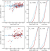 |
Fig. A.1 Comparison of the stellar metallicities taken from the NASA Exoplanet Archive (NEA) and homogeneously derived in SWET-Cat. The top and bottom panels show the results for the full and main samples, respectively. The brown symbols and curves represent the data for the Phigh stars and theskyblue symbols and curves for the Plow stars. The right panels show the CDFs of the metallicities for the Plow and Phigh stars. |
We cross-matched the full (1421 planets orbiting around 1058 stars) and the main (506 planets orbiting around 388 stars) samples of W20 with the SWEET-Cat (Santos et al. 2013; Sousa et al. 2018), which provides the stellar parameters of planet host stars. Although SWEET-Cat is one of the largest catalogs (and the largest one for the RV detected planets) of planet host stars with homogeneously determined stellar parameters, unfortunately it contains stellar parameters only for 375 stars from the full sample and 153 stars from the main sample of W20. In Figs. A.1 and A.2, we compare the stellar metallicities and masses presented in NEA and those that were homogeneously derived in SWEET-Cat (Santos et al. 2013). The mean difference and dispersion for metallicity is 0.01 ± 0.12 dex and 0.01 ± 0.10 dex for the full and main samples, respectively. For the stellar masses, the mean difference and dispersion is 0.0 ± 0.4 M⊙ and 0.0 ± 0.2 M⊙ for the full and main samples, respectively.
In the left panels of Figs. A.1 and A.2 for the Phigh and Plow stars, we compare the CDFs of metallicity and masses as taken from NEA and SWEET-Cat. We then performed a KS test to evaluate the similarities of the distributions. The PKS values for most of the cases are very similar. The exception is for the stellar metallicity for the main sample, where a significant difference of PKS is obtained for the NEA and SWEET-Cat values. Furthermore, if instead of the KS test, the AD test is performed to the aforementioned samples, the result would differ more dramatically (PAD = 0.03 and PAD > 0.25 for the SWEET-Cat and NEA metallicities, respectively), suggesting that the metallicity (taken from SWEET-Cat) distributions of the Phigh and Plow stars do not come from the same parent distribution.
Appendix B Stellar ages
For the sample of 178 FGK dwarf stars hosting 214 RV detected giant planets (see Sect. 2), we derived the stellar ages from the PARAM v1.3 web interface based on the Padova theoretical isochrones from Bressan et al. (2012) and with the use of a Bayesian estimation method (da Silva et al. 2006). As input parameters for PARAM, we used the Gaia DR2 parallaxes (Gaia Collaboration 2018), V magnitudes extracted from Simbad8, and spectroscopic Teff and [Fe/H]. No correction for interstellar reddening was needed since all the stars are nearby objects. The ages of all the stars are presented ina table at the CDS.
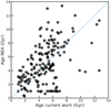 |
Fig. B.1 Comparison of the stellar ages taken from NEA and homogeneously derived in this work. The skyblue dashed line represents the identity line. |
Appendix C Supplementary figures
In Fig. B.1 we compare the ages homogeneously derived in this work and those from NEA. While there is practically no offset (−0.1 Gyr), the dispersion is 2.7 Gyr. The figure also shows a group of 13 stars with NEA ages of exactly 1 Gyr. Eight of these stars, however, have isochrone ages (as derived in this work) greater than 5 Gyr and are excluded from the main sample. All of these stars cool (Teff < 5350 K) and slightly evolved (logg < 4.4 dex), indicating their non-young ages.
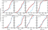 |
Fig. C.1 CDFs of different properties of planets and their host stars from the FGKPlow,high sample associated with over- (brown) and under-densities (skyblue). The PAD values for each parameter is shown in the respective plot. |
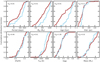 |
Fig. C.2 Same as Fig. C.1, but for the extended sample: stars with ages between 0.5 and 5 Gyr as well as the Phigh threshold of 0.30. |
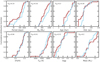 |
Fig. C.3 Same as Fig. C.1, but for a sample of stars with ages between 2.5 and 5 Gyr, planets with masses greater than 150 M⊕, and the Phigh threshold of 0.30. |
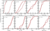 |
Fig. C.4 CDFs of different properties of short- (Period < 30 days; solid line) and long-period (Period > 30 days; dashed line) planets and their host stars from the extended FGKPlow,high sample associated with over-densities. The PAD values for each parameter is shown in the respective plot. |
References
- Adibekyan, V. 2019, Geosciences, 9, 105 [NASA ADS] [CrossRef] [Google Scholar]
- Adibekyan, V. Z., Figueira, P., Santos, N. C., et al. 2013, A&A, 560, A51 [NASA ADS] [CrossRef] [EDP Sciences] [Google Scholar]
- Astropy Collaboration (Price-Whelan, A. M., et al.) 2018, AJ, 156, 123 [Google Scholar]
- Bitsch, B., Trifonov, T., & Izidoro, A. 2020, A&A, 643, A66 [EDP Sciences] [Google Scholar]
- Bressan, A., Marigo, P., Girardi, L., et al. 2012, MNRAS, 427, 127 [NASA ADS] [CrossRef] [Google Scholar]
- Brucalassi, A., Pasquini, L., Saglia, R., et al. 2016, A&A, 592, L1 [NASA ADS] [CrossRef] [EDP Sciences] [Google Scholar]
- Buchhave, L. A., Bitsch, B., Johansen, A., et al. 2018, ApJ, 856, 37 [NASA ADS] [CrossRef] [Google Scholar]
- da Silva, L., Girardi, L., Pasquini, L., et al. 2006, A&A, 458, 609 [NASA ADS] [CrossRef] [EDP Sciences] [Google Scholar]
- Davies, M. B., Adams, F. C., Armitage, P., et al. 2014, in Protostars and Planets VI, eds. H. Beuther, R. S. Klessen, C. P. Dullemond, & T. Henning (Tucson: University of Arizona Press), 787 [Google Scholar]
- Dawson, R. I., & Johnson, J. A. 2018, ARA&A, 56, 175 [NASA ADS] [CrossRef] [Google Scholar]
- Dawson, R. I., & Murray-Clay, R. A. 2013, ApJ, 767, L24 [NASA ADS] [CrossRef] [Google Scholar]
- Gaia Collaboration (Brown, A. G. A., et al.) 2018, A&A, 616, A1 [NASA ADS] [CrossRef] [EDP Sciences] [Google Scholar]
- Goda, S., & Matsuo, T. 2019, ApJ, 876, 23 [Google Scholar]
- Hamer, J. H., & Schlaufman, K. C. 2019, AJ, 158, 190 [Google Scholar]
- Hatzes, A. P. 2016, Space Sci. Rev., 205, 267 [NASA ADS] [CrossRef] [Google Scholar]
- Hunter, J. D. 2007, Comput. Sci. Eng., 9, 90 [NASA ADS] [CrossRef] [Google Scholar]
- Kruijssen, J. M. D., Longmore, S. N., & Chevance, M. 2020, ApJ, 905, L18 [Google Scholar]
- Maldonado, J., Eiroa, C., Villaver, E., Montesinos, B., & Mora, A. 2012, A&A, 541, A40 [NASA ADS] [CrossRef] [EDP Sciences] [Google Scholar]
- Maldonado, J., Villaver, E., & Eiroa, C. 2013, A&A, 554, A84 [NASA ADS] [CrossRef] [EDP Sciences] [Google Scholar]
- Maldonado, J., Villaver, E., Eiroa, C., & Micela, G. 2019, A&A, 624, A94 [CrossRef] [EDP Sciences] [Google Scholar]
- Mordasini, C., Alibert, Y., Benz, W., & Naef, D. 2009, A&A, 501, 1161 [NASA ADS] [CrossRef] [EDP Sciences] [Google Scholar]
- Mortier, A., Santos, N. C., Sousa, S. G., et al. 2013, A&A, 557, A70 [NASA ADS] [CrossRef] [EDP Sciences] [Google Scholar]
- Osborn, A., & Bayliss, D. 2020, MNRAS, 491, 4481 [Google Scholar]
- Pettitt, A. N. 1976, Biometrika, 63, 161 [Google Scholar]
- Raymond, S. N., Armitage, P. J., & Gorelick, N. 2009, ApJ, 699, L88 [NASA ADS] [CrossRef] [Google Scholar]
- Saculinggan, M., & Balase, E. A. 2013, J.. Phys. Conf. Ser., 435, 012041 [Google Scholar]
- Santos, N. C., Sousa, S. G., Mortier, A., et al. 2013, A&A, 556, A150 [NASA ADS] [CrossRef] [EDP Sciences] [Google Scholar]
- Santos, N. C., Adibekyan, V., Figueira, P., et al. 2017, A&A, 603, A30 [NASA ADS] [CrossRef] [EDP Sciences] [Google Scholar]
- Shara, M. M., Hurley, J. R., & Mardling, R. A. 2016, ApJ, 816, 59 [Google Scholar]
- Sotiriadis, S., Libert, A.-S., Bitsch, B., & Crida, A. 2017, A&A, 598, A70 [NASA ADS] [CrossRef] [EDP Sciences] [Google Scholar]
- Sousa, S. G., Santos, N. C., Mayor, M., et al. 2008, A&A, 487, 373 [NASA ADS] [CrossRef] [EDP Sciences] [MathSciNet] [Google Scholar]
- Sousa, S. G., Adibekyan, V., Delgado-Mena, E., et al. 2018, A&A, 620, A58 [NASA ADS] [CrossRef] [EDP Sciences] [Google Scholar]
- Sozzetti, A. 2004, MNRAS, 354, 1194 [CrossRef] [Google Scholar]
- Stock, K., Cai, M. X., Spurzem, R., Kouwenhoven, M. B. N., & Portegies Zwart, S. 2020, MNRAS, 497, 1807 [Google Scholar]
- van der Walt, S., Colbert, S. C., & Varoquaux, G. 2011, Comput. Sci. Eng., 13, 22 [Google Scholar]
- Vincke, K., & Pfalzner, S. 2018, ApJ, 868, 1 [NASA ADS] [CrossRef] [Google Scholar]
- Virtanen, P., Gommers, R., Oliphant, T. E., et al. 2020, Nat. Methods, 17, 261 [Google Scholar]
- Wang, J., Fischer, D. A., Horch, E. P., & Huang, X. 2015, ApJ, 799, 229 [NASA ADS] [CrossRef] [Google Scholar]
- Wang, Y.-H., Leigh, N. W. C., Perna, R., & Shara, M. M. 2020, ApJ, 905, 136 [Google Scholar]
- Wes McKinney. 2010, in Proceedings of the 9th Python in Science Conference, ed. Stéfan van der Walt, & Jarrod Millman, 56 [Google Scholar]
- Winn, J. N., & Fabrycky, D. C. 2015, ARA&A, 53, 409 [Google Scholar]
- Winter, A. J., Kruijssen, J. M. D., Longmore, S. N., & Chevance, M. 2020, Nature, 586, 528 [Google Scholar]
The definition of HJs in terms of the upper limit of the orbital period (or semi-major axis) and the lower limit in planetary mass (or radius) varies in the literature.
Transiting planets have only short periods and are not suitable for our analysis.
AD is similar to the Kolmogorov–Smirnov (KS) test, but it is more sensitive to the tails of distribution and has higher power for small samples (Pettitt 1976; Saculinggan & Balase 2013).
We note that due to the constraint on the homogeneity of the stellar parameters, only ten stars (i.e., 5%) have been excluded at this stage.
The stars with Phigh > 0.84 are called Phigh, and the stars with Phigh < 0.16 are called Plow.
By adopting an upper limit of 0.2 AU for the semi-major axis of HJs, Winter et al. (2020) limited their sample to planets with orbital periods shorter than about 30 days.
All Figures
|
Fig. 1 Distribution of the RV detected planets on the period-mass diagram orbiting around FGK dwarf stars with homogeneously derived stellar parameters in SWEET-Cat. The left panel is for the FGKPlow,high sample and the right panel is for the planets in the expended sample. |
| In the text | |
|
Fig. 2 Fraction of HJs orbiting cluster (brown) and field (skyblue) stars as a function of Phigh threshold which is used to separate the aforementioned two groups. The numbers next to the HJs fraction correspond to the numbers of HJs and the total number of planets that are used to compute these fractions. The upperlimit for the HJs orbital period was set at 10 (top), 20 (middle), and 30 (bottom) days. The PAD values on top of the panels show the results of the AD test comparing the distributions of the ages of the cluster and field stars. The errorbars represent a 68.3% (1σ) interval. |
| In the text | |
|
Fig. 3 Fraction of HJs orbiting cluster (brown) and field (skyblue) stars as a function of upper age limit. The lower age limit is set to 0.5 Gyr and the Phigh threshold was set to 0.3. The symbols and numbers are the same as in Fig. 2. |
| In the text | |
|
Fig. 4 Period-mass diagram of planets around FGK Phigh (left panel) and Plow (right panel) dwarf stars with homogeneously derived stellar parameters in SWEET-Cat. Only stars with ages between 1 and 4.5 Gyr are shown. Planets orbiting metal-poor and metal-rich stars are shown in open and filled circles, respectively. |
| In the text | |
|
Fig. A.1 Comparison of the stellar metallicities taken from the NASA Exoplanet Archive (NEA) and homogeneously derived in SWET-Cat. The top and bottom panels show the results for the full and main samples, respectively. The brown symbols and curves represent the data for the Phigh stars and theskyblue symbols and curves for the Plow stars. The right panels show the CDFs of the metallicities for the Plow and Phigh stars. |
| In the text | |
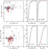 |
Fig. A.2 Same as Fig. A.1, but for stellar masses. |
| In the text | |
|
Fig. B.1 Comparison of the stellar ages taken from NEA and homogeneously derived in this work. The skyblue dashed line represents the identity line. |
| In the text | |
|
Fig. C.1 CDFs of different properties of planets and their host stars from the FGKPlow,high sample associated with over- (brown) and under-densities (skyblue). The PAD values for each parameter is shown in the respective plot. |
| In the text | |
|
Fig. C.2 Same as Fig. C.1, but for the extended sample: stars with ages between 0.5 and 5 Gyr as well as the Phigh threshold of 0.30. |
| In the text | |
|
Fig. C.3 Same as Fig. C.1, but for a sample of stars with ages between 2.5 and 5 Gyr, planets with masses greater than 150 M⊕, and the Phigh threshold of 0.30. |
| In the text | |
|
Fig. C.4 CDFs of different properties of short- (Period < 30 days; solid line) and long-period (Period > 30 days; dashed line) planets and their host stars from the extended FGKPlow,high sample associated with over-densities. The PAD values for each parameter is shown in the respective plot. |
| In the text | |
Current usage metrics show cumulative count of Article Views (full-text article views including HTML views, PDF and ePub downloads, according to the available data) and Abstracts Views on Vision4Press platform.
Data correspond to usage on the plateform after 2015. The current usage metrics is available 48-96 hours after online publication and is updated daily on week days.
Initial download of the metrics may take a while.