| Issue |
A&A
Volume 646, February 2021
|
|
|---|---|---|
| Article Number | A176 | |
| Number of page(s) | 7 | |
| Section | Galactic structure, stellar clusters and populations | |
| DOI | https://doi.org/10.1051/0004-6361/202040038 | |
| Published online | 23 February 2021 | |
Signatures of tidal disruption in the Milky Way globular cluster NGC 6981 (M72)
1
Instituto Interdisciplinario de Ciencias Básicas (ICB), CONICET-UNCUYO, Padre J. Contreras 1300, M5502JMA Mendoza, Argentina
e-mail: andres.piatti@unc.edu.ar
2
Consejo Nacional de Investigaciones Científicas y Técnicas (CONICET), Godoy Cruz 2290, C1425FQB Buenos Aires, Argentina
3
Instituto de Astrofísica de La Plata (CONICET-UNLP), Buenos Aires, Argentina
4
Facultad de Ciencias Astronómicas y Geofísicas de La Plata (UNLP), La Plata, Argentina
5
Instituto de Alta Investigación, Universidad de Tarapacá, Casilla 7D, Arica, Chile
6
European Southern Observatory, Alonso de Córdova 3107, Casilla, 19001 Santiago, Chile
7
Millenium Institute of Astrophysics, Av. Vicuña Mackenna 4860, 782-0436 Macul, Santiago, Chile
8
Instituto de Astrofísica, Facultad de Física, Pontificia Universidad Católica de Chile, Av. Vicuña Mackenna 4860, 782-0436 Macul, Santiago, Chile
Received:
1
December
2020
Accepted:
4
January
2021
We study the outer regions of the Milky Way globular cluster NGC 6981 based on publicly available BV photometry and new Dark Energy Camera (DECam) observations, both of which reach nearly 4 mag below the cluster main sequence (MS) turnoff. While the BV data sets reveal the present of extra-tidal features around the cluster, the much larger field of view of the DECam observations allowed us to identify some other tidal features, which extend from the cluster toward the opposite direction to the Milky Way center. Such structural features of clusters arise from stellar density maps built using MS stars, following a cleaning of the cluster color-magnitude diagram to remove the contamination of field stars. We also performed N-body simulations in order to help us to understand the spatial distribution of the extra-tidal debris. The outcomes reveal the presence of long trailing and leading tails that are mostly parallel to the direction of the cluster velocity vector. We find that the cluster loses most of its mass by tidal disruption during its perigalactic passages, each of which lasted nearly 20 Myr. Hence, a decrease in the density of escaping stars near the cluster is expected from our N-body simulations, which, in turn, means that stronger extra-tidal features could be found by exploring much larger areas around NGC 6891.
Key words: globular clusters: individual: NGC 6981 / globular clusters: general / techniques: photometric / methods: numerical
© ESO 2021
1. Introduction
Globular clusters, formed in external galaxies and then gravitationally stripped off by the Milky Way and usually called accreted globular clusters, are expected to show evidence of extra-tidal features, such as tidal tails, azimuthally irregular stellar halos, and clumpy extended structures (Carballo-Bello et al. 2014; Vanderbeke et al. 2015; Kuzma et al. 2016; Piatti & Carballo-Bello 2020). Over the last few years, sufficiently deep wide-sky photometric surveys have allowed us to explore the outermost regions of a number of globular clusters, resulting in the detection of a variety of extra-tidal structures around them. For instance, tidal tails were very recently identified in NGC 362 (Carballo-Bello 2019), NGC 1851, NGC 2808 (Carballo-Bello et al. 2018; Sollima 2020), 4590 (Palau & Miralda-Escudé 2019), 5139 (Ibata et al. 2019), 5904 (Grillmair 2019), and others. These globular clusters are now expanding the list of now nearly 15 globular clusters which have detected tidal tails (e.g., Pal 5; Odenkirchen et al. 2001).
Koppelman et al. (2019) associated seven globular clusters with the accreted Helmi streams (Helmi et al. 1999) based on their kinematic properties: NGC 4590, 5024, 5053, 5272, 5634, 5904, and 6981. Massari et al. (2019) added Pal 5, Rup 106, and E 3 in the candidates list based on their orbital properties and a less restrictive set of selection criteria. However, the membership of E 3 to this group was recently questioned by Forbes (2020). All of them have prograde orbital motions and according to the recent classification of globular clusters carried out by Piatti & Carballo-Bello (2020) from studies focused on their outermost regions, we find (among those associated to the Helmi streams) three globular clusters with observed tidal tails (NGC 4590, 5904, Pal 5), two with extra-tidal features that are different from tidal tails (NGC 5053, 5634), and three without any signatures of extended stellar density profiles (NGC 5024, 5272, Rup 106). Recently, Carballo-Bello et al. (2020) confirmed the presence of tidal tails emerging from E 3 using Gaia DR2 data. The outermost regions of NGC 6981 have been studied by Grillmair et al. (1995) from photographic photometry that reaches down the main sequence turnoff (see, also, Amigo et al. 2013). They estimated a tidal radius of 8.3′ and did not find any signature of clear tidal tails.
NGC 6981 is identified as lying on a sequence of possibly accreted globular clusters in the age-metallicity diagram, which coincides with the Kraken clusters (Kruijssen et al. 2019). As can be inferred, the different proposed progenitors of NGC 6981 points to the need for further refinement in the different selection procedures (Piatti 2019). The ratios of the cluster mass lost by tidal disruption of the Milky Way gravitation field to the initial cluster mass (Mdis/Mini) computed by Piatti et al. (2019) result to be relatively small for the 6 Helmi streams globular clusters mentioned by Koppelman et al. (2019) with studies of their outermost regions (0.04 ≤ Mdis/Mini ≤ 0.15). Pal 5 and Rup 106 have Mdis/Mini = 0.24, while NGC 6981, 0.41. The Mdis/Mini ratio was used by Piatti et al. (2019) as an indicator of tidal field strength. They studied the relationship between Mdis/Mini, the semimajor axes and the eccentricity of the globular clusters’ orbits (see their Fig. 1) and found that clusters with relatively high Mdis/Mini are either clusters with orbit eccentricities ≳0.7 or semimajor axes ≲3 kpc. Nevertheless, a puzzling population of clusters with intermediate eccentricities and short semimajor axes is observed, also with relatively high orbital inclinations.
In this study, we focus on NGC 6981 with the aim of finding trails of tidal tails that can explain the large amount of mass lost by the interaction with the Milky Way gravitational field. In Sect. 2, we describe the analysis carried out on the basis of public data sets, while in Sect. 3 we perform a similar analysis based on our own, more spatially extended observations. Section 4 discusses the present outcomes, while Sect. 5 summarizes the main conclusions of this work.
2. Public data handing
We searched for unexplored public wide-field photometry that is widely available in order to build stellar density maps from faint cluster main sequence (MS) stars that are suitable for uncovering extra-tidal structures. The homogeneous Johnson BV photometry published by Stetson et al. (2019) for NGC 6981, with typical internal and external uncertainties of the order of a few millimagnitudes, turned out to be the most appropriate one. The field-of-view is  , centered on the cluster, which allows us to examine out to nearly twice the cluster tidal radius (
 ; Harris 1996, 2010 Edition). The reddening variation across the cluster field is shown in Fig. 1, with E(B − V) color excess retrieved from Schlafly & Finkbeiner (2011) provided by the NASA/IPAC Infrared Science Archive1. Although the cluster field is not affected by differential reddening, we preferred to employ dereddened color-magnitude diagrams (CMDs) by correcting the V mags and B − V colors using the E(B − V) color excesses associated to the positions of the stars in the sky. Figure 2 shows the intrinsic CMDs for a cluster region (
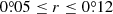 ) compared to a star field region with equal cluster area, located far from the cluster.
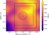 |
Fig. 1. Reddening variation across the field of NGC 6981. The solid box represents the area of the Stetson et al. (2019)’s photometry, while the dashed lines delimit the internal boundaries of the adopted field star reference field. The circle corresponds to the cluster tidal radius compiled by Harris (1996). |
We devised two segments along the cluster MS (see Fig. 2) where we perform star counts. Both segments are contaminated by the presence of field stars, so that we first applied the procedure proposed by Piatti & Bica (2012) to statistically eliminate them. The method compares the distribution of MS stars within the devised segments, spread across the cluster field, with that of a reference star field. For this purpose, we adopted as a reference star field the area delimited by the dashed lines in Fig. 1 and the data set boundary, where we assumed that the stellar density, and the distribution in V mag and B − V colors of those stars are representative of the field stars projected along the line-of-sight of the cluster. We subtract from each segment a number of stars equal to the corresponding one in the reference star field. The distribution of magnitudes and colors of the subtracted stars from the cluster CMD needs to resemble that of the reference star field. With the aim of avoiding stochastic effects caused by very few field stars distributed in less populated CMD regions, we started finding stars to eliminate within a cell of (ΔV0, Δ(B − V)0) = (1.0 mag,0.5 mag) centered on the magnitude and color values of each reference field star. Thus, it is highly probable that we may find a star in the cluster CMD with (V0, (B − V)0) values within those boundaries around those (V0, (B − V)0) of each field star. In the case when more than one star is located inside a cell, the closest one to the center of that (V0, (B − V)0) cell is subtracted. The photometric errors are also taken into account while searching for a star to be subtracted from the cluster CMD. To that purpose, we iterate up to one thousand times the comparison between the (V0, (B − V)0) values of the reference field star and those of the stars in the cluster CMD. If a star in the cluster CMD falls inside the defined cell for the reference field star, we subtract that star. The iterations were carried out by allowing the (V0, (B − V)0) values of the star in the cluster CMD takes smaller or larger values than the mean ones according to their respective errors.
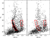 |
Fig. 2. Intrinsic CMDs for the cluster field (left panel) for an annulus with internal and external radii of |


Figure 3 (upper panels) depicts the observed stellar density maps built for the two MS segments using the scikit-learn software machine learning library (Pedregosa et al. 2011) and its Gaussian kernel density estimator (KDE). We employed a grid of 100 × 100 boxes onto the cluster area and used a range of values for the bandwidth from 0.005° up to 0.040° in steps of 0.005° in order to apply the KDE to each generated box. We adopted a bandwidth of 0.020° as the optimal value, as guided by scikit-learn. We also estimated the background level using the stars distributed within the reference field star area. We divided this area in boxes of  and counted the number of stars inside them. We randomly shifted the boxes by
  along the right ascension (RA) and declination (Dec) directions and repeated the star counting. Finally, we derived the mean value using all the defined boxes. As for the standard deviation, we performed a thousand Monte Carlo realizations using the stars located in the reference field star area, which were shifted along Δ(RA)×cos(Dec) or Δ(Dec) randomly (one different shift for each star) before recomputing the density map. The color scale in Fig. 3 represents the absolute deviation from the mean value in the field in units of the standard deviation, that is, η = (signal − mean value)/standard deviation. We have painted white stellar densities with η > 10 in order to highlight the least dense structures.
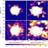 |
Fig. 3. Observed (upper panels) and field star cleaned (bottom panels) stellar density maps for the brighter (left panels) and the fainter (right panels) cluster MS segments according to Fig. 2. The black circle centered on the cluster indicates the cluster tidal radius. Contours for η = 3, 5, 7, and 9 are also shown, reflecting significance levels. |
We additionally considered the devised segment located to redder colors in the cluster CMD (the box centered at (B − V)0 ≈ 1.5 mag), which represents a composite field star population, and applied the same cleaning procedure. We found that the resulting cleaned stellar density map does not contain any visible structure above 1η, which means that the residuals of the cleaning technique are negligible. Therefore, we assume that any stellar enhancement remaining in the stellar density maps built from the cleaned cluster CMD is an intrinsic cluster feature. The resulting field star decontaminated stellar density maps are shown in the bottom panels of Fig. 3, where extra-tidal features are readily visible. As expected, more extended extra-tidal features show up in the case of the lowest-mass segment, as lower-mass stars can be more easily stripped away from the cluster than their higher-mass counterparts.
3. Data collection and processing
With the aim of tracing the cluster extra-tidal features farther out, we carried out observations (program ID : 2019B-1003) with the Dark Energy Camera (DECam), attached to the prime focus of the 4-m Blanco telescope at Cerro Tololo Inter-American Observatory (CTIO). DECam provides a 3 deg2 field of view (see Fig. 4) with its 62 identical chips with a scale of 0.263 arcsec pixel−1 (Flaugher et al. 2015). We observed NGC 6981 with the g and r bands, for which we obtained 4 exposures of 600 s. and 400 s, respectively. We also observed 3–5 SDSS fields per night at a different airmass to derive the atmospheric extinction coefficients and the transformations between the instrumental magnitudes and the SDSS ugriz system (Fukugita et al. 1996).
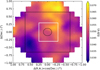 |
Fig. 4. Reddening variation across the DECam field of NGC 6981. The solid white box represents the area of the Stetson et al. (2019)’s photometry (see Fig. 1), while black circle and box represent the cluster tidal radius compiled by Harris (1996), and the internal boundary of the adopted field star reference field. |
We processed the images using the DECam Community Pipeline (Valdes et al. 2014), while the photometry was obtained from the images with the PSF-fitting algorithm of DAOPHOT II/ALLSTAR (Stetson 1987). The final catalog includes only stellar-shaped objects with |sharpness| ≤ 0.5 to avoid (as much as possible) the presence of non-stellar sources and background galaxies in our analysis. In addition, DAOPHOT II was used to add synthetic stars in our images in order to estimate the completeness of our photometric catalogs. After applying our photometry pipeline on the images with the created artificial stars included, we found that the magnitude for a 50% recovery of the artificial stars added turned out to be 23.4 mag and 23.3 mag for the g and r bands, respectively.
The methodology that we employed to build the stellar density maps followed the steps described in Sect. 2. We obtained the reddening free g0 magnitudes and (g − r)0 colors by using the individual E(B − V) values (see Fig. 4) and the Aλ/AV coefficients given by Wang & Chen (2019). Figure 5 illustrates the cluster CMD we obtained for the main body of the cluster. Two different segments were devised along the cluster MS and the field star cleaning procedure was applied. In this case, we used as the reference star field the region located outside the large black box drawn in Fig. 4. Because of the larger area of the DECam FOV with respect to Stetson et al. (2019)’s FOV, we thoroughly monitor the performance of the cleaning procedure by repeating the search for a star to be subtracted in the cluster area for each star in the reference star field a thousand times. The position of the subtracted star in the cluster field was chosen randomly during each simulation of the cleaning procedure. We finally kept those stars that remained unsubtracted more than 50% of the total number of cleaning runs. The observed and field star cleaned stellar density maps for both MS segments are depicted in Fig. 6.
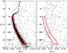 |
Fig. 5. Same as Fig. 2 for the present DECam photometry. Two segments along the cluster MS are indicated with red lines. Error bars are also shown. |
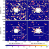 |
Fig. 6. Observed (upper panels) and field star cleaned (bottom panels) stellar density maps for the brighter (left panels) and the fainter (right panels) cluster MS segments according to Fig. 4. The black circle centered on the cluster indicates the cluster tidal radius, while the white box represents the area of the Stetson et al. (2019)’s photometry (see Fig. 1). Contours for η = 3, 5, 7, and 9 are also shown. Gray and white arrows represent the direction of the motion of the cluster and that toward the Galactic center, respectively. |
4. Analysis and discussion
Figure 6 shows that NGC 6981 has visible extra-tidal structures, which can be described as a non-rounded extended halo and debris distributed along the trailing tail. Piatti et al. (2019) computed the Jacobi radii of the cluster for its peri (1.3 kpc) and apogalactic (26.6 kpc) distances (Baumgardt et al. 2019), which resulted to be 15.5 pc and 67.7 pc, respectively. If we considered the present cluster Galactocentric distance of 12.85 kpc, its Jacobi radius would be ∼39.0 pc, or  for its heliocentric distance of 17.0 kpc. This Jacobi radius turned out to be similar to the tidal radius compiled by Harris (1996) and it is indicated with a black circle in Fig. 6. According to the semianalitical model in Piatti et al. (2019), who assumed a 50% cluster mass loss by evolutionary effects (see their Eq. (5) and also Baumgardt et al. (2019)), the amount of cluster mass lost by tidal disruption increases up to 41% of its initial cluster mass, which means that the present remaining mass of NGC 6981 is nearly 9% of its initial cluster mass.
The stellar density map built by Grillmair et al. (1995) for NGC 6981 using stars distributed in an area of ∼3 reveals the presence of some low-level stellar residuals beyond the cluster tidal radius. Although the authors did not draw a conclusion regarding the existence of tidal tails, their density map hints at some extra-tidal structure aligned toward the opposite direction to the Milky Way center. We note that they used a much shallower photometry than what we have for this work.
We performed N-body simulations to investigate the expected tidal features generated only during the last pericentric passages, that is, the last 2 Gyr of evolution, because we do not know how long the cluster has been following the present orbit. We first put a test particle representing the globular cluster at its present position and with its present center of mass velocity and integrated it backwards in time for a gravitational field model of the Milky Way. Then we replaced the test particle with an N-body system representing the globular cluster and integrated it forward in time up to the present epoch, keeping it embedded in the same host gravitational field. At this point, the tidal features developed by the cluster can be compared with those that have been observed.
Following Baumgardt et al. (2019), we modeled the Milky Way with Model I of Irrgang et al. (2013), consisting of a bulge, a disk, and a halo component. In order to compute the initial conditions at the present epoch, we used Astropy (Astropy Collaboration 2013, 2018) to convert the observed RA, Dec, distance, radial velocity, and proper motions given in Table 1 of Baumgardt et al. (2019) to Galactocentric coordinates. We adopted a Cartesian reference frame (X, Y, Z) with corresponding velocities (U, V, W) in which the X and U axes point from the Galactic center towards the opposite direction of the Sun; Y and V point in the direction of the Galactic rotation at the location of the Sun; and Z and W point towards the North Galactic Pole. We note that this right-handed frame of reference differs from the left-handed one used by Baumgardt et al. (2019). We assumed a distance from the Sun to the Galactic center of d = 8.1 kpc (GRAVITY Collaboration 2018) and a velocity of the Sun respect to the Galactocentric frame of (U, V, W)⊙ = (11.1, 252.24, 7.25) km s−1 in agreement with Schönrich et al. (2010) and Reid & Brunthaler (2004). The resulting Cartesian coordinates are listed in Table 1.
Present position and velocity of NGC 6981 in Galactocentric coordinates, used as initial conditions for the backwards (Δt < 0) test particle integration.
From these initial conditions, we integrated the equations of motion backwards in time during 1.9 Gyr, an interval chosen in order to start the forward integration near the apocenter of the orbit. Figure 7 shows the projection on the Y − Z plane of this backward orbit, where we can see a clear 3 : 2 resonance (a “fish”). The orbit precesses around the Z-axis.
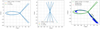 |
Fig. 7. Orbit of the test particle in the Y − Z (left panel) and X − Y (middle panel) planes, respectively. Present N-body snapshot (blue) and orbit of the test particle (green) in the Y − Z plane (right panel). The point of highest density of the N-body cluster is marked in red. The black arrow is parallel to the velocity of the globular cluster projected in the Y − Z plane. |
During the Y > 0 portions of the orbit, the cluster moves almost radially (eccentricity e ≤ 1) deep into the halo with an inclination ∼45° with respect to the Milky Way plane. During the Y < 0 portions, the cluster loops perpendicularly to the disk with e > 0. As the pericentric distance is only ≲1 kpc, the details of the integrated orbit may not coincide with those of the real one, in the sense that phenomena such as dynamical friction are not taken into account in a test particle integration.
The globular cluster was modeled with an initial King profile (King 1966) of total mass M = 2 × 10⁵ M⊙; a King radius, r0 = 2.8 pc; a King concentration parameter, cK = log10(rt/r0) = 1.183; and a central potential, W0 = 5.7, using N = 5 × 10⁴ stars of 4 solar masses. With these values, other important parameters are: tidal radius, rt = 42.64 pc; core radius, rc = 2.29 pc; and a concentration parameter, c = log10(rt/rc) = 1.27. This initial parameters are in agreement with those compiled by Harris (1996) and Baumgardt et al. (2019), which are respectively c = 1.23 and rc = 2.33 pc. By fitting these parameters at the end of the simulation would have required probing initial values in a trial-and-error approach; therefore, we chose to fix them at the start of the simulation.
The cluster was placed at the final position of the backward integration and then evolved forward with the code Gadget-2 (Springel 2005), using a maximum step size of 0.01 Myr and a softening length of 0.5 pc. We used a version of the code that allows external potentials to be included in the simulation, in our case, that of the Galaxy. Also, the adaptive time-step criterion takes into account the presence of this potential (Villalobos & Helmi 2008, Appendix A2.3). Taking into account that the cluster losses mass in this forward integration due to tidal forces, the value of the initial mass, M, was chosen so that the final mass was close to the observed mass, Mobs = 8.7 × 10⁴ M⊙ (Baumgardt et al. 2019). In the simulation, the final mass turned out to be Mf = 9.2 × 10⁴ M⊙. The difference between the mass loss from the simulation and that of the semianalytical model is expected given that they are based on different methodologies and hypothesis. We use “present” to refer to the characteristics of this final state.
Figure 7 shows that a large stellar stream with both leading and trailing tails has formed, which explores both disk and halo regions. The point of highest density in the present N-body cluster was approximated as follows. We started computing the center of mass of all the particles inside a box with edges rbox = 50rc, centered at the origin of coordinates. Then we computed a new center of mass by choosing the particles that lie inside a box with an edge that is one percent smaller than the previous one, centered at the previous center of mass. Then we iterated this last step two hundred times. The resulting center of mass turned out to be a good approximation to the density peak of the distribution. The regions close to the present N-body snapshot, projected onto the three coordinate planes are depicted in Fig. 8. The offset of the present position of NGC 6981, with respect to the point of highest density of the N-body simulation is as expected: the backward orbit of the test particle initialized at the position of NGC 6981 is followed forward approximately by the center of mass of the full set of N-body particles, which does not coincide with their peak density due to the streams. Figure 9 shows the mass of the N-body cluster inside a radius equal to the initial tidal radius M(r < rt), as a function of time. It is readily visible that the cluster loses stars only at its pericentric passages during approximately 20 Myr.
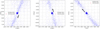 |
Fig. 8. Present N-body snapshot (blue) in the X − Y, X − Z, and Y − Z planes. The point of highest density of the N-body cluster is marked in red. The black arrow is parallel to the velocity of NGC 6981 in projected plane. |
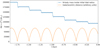 |
Fig. 9. Mass evolution (blue dotted line) and Galactocentric distance in arbitrary units (solid orange line) of the N-body cluster. |
To compare the distribution of the N-body particles with the observed stellar density (see Fig. 6), we projected the former into the celestial sphere and computed the surface mass density Σ(Δ((RA)cos(Dec),Δ(Dec)), where Δ(RA) and Δ(Dec) are the RA and Dec of a point of the sphere with respect to the position of the highest density peak of the N-body cluster. In order to highlight the density variations, we have applied an upper threshold value of Σthres = 5000 M⊙ deg−2; all the pixels above this value were colored in white. Figure 10 shows that the tidal tails extend towards the North-East and the South-West directions, respectively. Notwithstanding the clear streams in the larger fields, they seem to have disappeared in the smallest one. This is due to the fact that the stream slowly drifts from the cluster, and the mass loss only happens during very short intervals at the pericenter passages. Therefore, we expect a gap of streaming stars near the cluster, widening between pericenter passages.
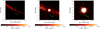 |
Fig. 10. Surface density of the N-body cluster on the celestial sphere. The arrow is parallel to the measured proper motion vector corrected by the solar reflex motion with the Gala code (Price-Whelan 2017). The right panel can be directly compared to Fig. 6. |
5. Conclusions
In this work, we analyze the outer regions of the Milky Way globular cluster NGC 6981 with the aim of identifying extra-tidal features. The cluster caught our attention because it was associated to the accreted Helmi streams and deposited in an extremely inner halo orbit, with a relatively high eccentricity and inclination angle with respect to the Milky Way plane in the current orbital section. According to Piatti et al. (2019), globular clusters with orbital parameters similar to those of NGC 6981 have lost relatively more mass by tidal disruption than globular clusters rotating in the Milky Way disk.
We started by analyzing BV public data sets, which revealed the presence of extra-tidal debris distributed around the cluster. Our DECam observations, which reach nearly 4 mag below the cluster MS turnoff, confirmed our findings from a wider field of view. The BV and DECam photometries were treated similarly. We relied on MS stars, particularly the fainter ones because they are the first to cross the Jacobi radius once they reach the cluster boundary driven by two-body relaxation. Indeed, we found that the fainter the range of magnitudes considered, the more extended the cluster stellar density map.
In order to monitor any differential change in the stellar density map caused by cluster stars with distinct brightness, we split the long MS of the cluster into two segments of 2 and 1.5 mag long, respectively, and we analyzed them individually. The magnitudes and colors of the stars were corrected by individual interstellar reddening, which slightly varies across the field. Then we statistically decontaminated the cluster MS segments from the presence of field stars and built stellar density maps using all the stars that remained unsubtracted after the cleaning procedure. We built their respective stellar density maps using a kernel estimator technique, which revealed the presence of extra-tidal features oriented along the opposite direction to the Milky Way center.
N-body simulations were finally performed to help us to understand the spatial distribution of the extra-tidal debris. In our simulations, the cluster was represented by an N-body system that had evolved over 2 Gyr in the adopted Milky Way potential. The disrupted stars are clearly shown to form long trailing and leading tails, which are mostly parallel to the direction of the cluster velocity vector – this is similar to the direction pointing to the Galaxy centre at the present time. We confirmed a decrease in the density of extra-tidal stars near the cluster. In addition, we found that stronger extra-tidal features could be found by exploring larger areas around NGC 6891.
Acknowledgments
M.F.M. and D.C. acknowledge support from the Universidad Nacional de La Plata (grant 11/G153). M.F.M. thanks Juan Ignacio Rodriguez for maintaining the IALP server where the N-body code was run. M.D.M. thanks to the postdoctoral position CONICYT-GEMINI. We thank the referee for the thorough reading of the manuscript and timely suggestions to improve it. Based on observations at Cerro Tololo Inter-American Observatory, NSF’s NOIRLab (Prop. ID 2019B-1003; PI: Carballo-Bello), which is managed by the Association of Universities for Research in Astronomy (AURA) under a cooperative agreement with the National Science Foundation. This project used data obtained with the Dark Energy Camera (DECam), which was constructed by the Dark Energy Survey (DES) collaboration. Funding for the DES Projects has been provided by the US Department of Energy, the US National Science Foundation, the Ministry of Science and Education of Spain, the Science and Technology Facilities Council of the United Kingdom, the Higher Education Funding Council for England, the National Center for Supercomputing Applications at the University of Illinois at Urbana-Champaign, the Kavli Institute for Cosmological Physics at the University of Chicago, Center for Cosmology and Astro-Particle Physics at the Ohio State University, the Mitchell Institute for Fundamental Physics and Astronomy at Texas A&M University, Financiadora de Estudos e Projetos, Fundação Carlos Chagas Filho de Amparo à Pesquisa do Estado do Rio de Janeiro, Conselho Nacional de Desenvolvimento Científico e Tecnológico and the Ministério da Ciência, Tecnologia e Inovação, the Deutsche Forschungsgemeinschaft and the Collaborating Institutions in the Dark Energy Survey. The Collaborating Institutions are Argonne National Laboratory, the University of California at Santa Cruz, the University of Cambridge, Centro de Investigaciones Enérgeticas, Medioambientales y Tecnológicas–Madrid, the University of Chicago, University College London, the DES-Brazil Consortium, the University of Edinburgh, the Eidgenössische Technische Hochschule (ETH) Zürich, Fermi National Accelerator Laboratory, the University of Illinois at Urbana-Champaign, the Institut de Ciències de l’Espai (IEEC/CSIC), the Institut de Física d’Altes Energies, Lawrence Berkeley National Laboratory, the Ludwig-Maximilians Universität München and the associated Excellence Cluster Universe, the University of Michigan, NSF’s NOIRLab, the University of Nottingham, the Ohio State University, the OzDES Membership Consortium, the University of Pennsylvania, the University of Portsmouth, SLAC National Accelerator Laboratory, Stanford University, the University of Sussex, and Texas A&M University.
References
- Amigo, P., Stetson, P. B., Catelan, M., Zoccali, M., & Smith, H. A. 2013, AJ, 146, 130 [NASA ADS] [CrossRef] [Google Scholar]
- Astropy Collaboration (Robitaille, T. P., et al.) 2013, A&A, 558, A33 [NASA ADS] [CrossRef] [EDP Sciences] [Google Scholar]
- Astropy Collaboration (Price-Whelan, A. M., et al.) 2018, AJ, 156, 123 [Google Scholar]
- Baumgardt, H., Hilker, M., Sollima, A., & Bellini, A. 2019, MNRAS, 482, 5138 [Google Scholar]
- Carballo-Bello, J. A. 2019, MNRAS, 486, 1667 [NASA ADS] [CrossRef] [Google Scholar]
- Carballo-Bello, J. A., Sollima, A., Martínez-Delgado, D., et al. 2014, MNRAS, 445, 2971 [NASA ADS] [CrossRef] [Google Scholar]
- Carballo-Bello, J. A., Martínez-Delgado, D., Navarrete, C., et al. 2018, MNRAS, 474, 683 [NASA ADS] [CrossRef] [Google Scholar]
- Carballo-Bello, J. A., Salinas, R., & Piatti, A. E. 2020, MNRAS, 499, 2157 [Google Scholar]
- Flaugher, B., Diehl, H. T., Honscheid, K., et al. 2015, AJ, 150, 150 [Google Scholar]
- Forbes, D. A. 2020, MNRAS, 493, 847 [NASA ADS] [CrossRef] [Google Scholar]
- Fukugita, M., Ichikawa, T., Gunn, J. E., et al. 1996, AJ, 111, 1748 [NASA ADS] [CrossRef] [Google Scholar]
- GRAVITY Collaboration (Abuter, R., et al.) 2018, A&A, 615, L15 [NASA ADS] [CrossRef] [EDP Sciences] [Google Scholar]
- Grillmair, C. J. 2019, ApJ, 884, 174 [NASA ADS] [CrossRef] [Google Scholar]
- Grillmair, C. J., Freeman, K. C., Irwin, M., & Quinn, P. J. 1995, AJ, 109, 2553 [NASA ADS] [CrossRef] [Google Scholar]
- Harris, W. E. 1996, AJ, 112, 1487 [NASA ADS] [CrossRef] [Google Scholar]
- Helmi, A., White, S. D. M., de Zeeuw, P. T., & Zhao, H. 1999, Nature, 402, 53 [NASA ADS] [CrossRef] [Google Scholar]
- Ibata, R. A., Bellazzini, M., Malhan, K., Martin, N., & Bianchini, P. 2019, Nat. Astron., 3, 667 [NASA ADS] [CrossRef] [Google Scholar]
- Irrgang, A., Wilcox, B., Tucker, E., & Schiefelbein, L. 2013, A&A, 549, A137 [NASA ADS] [CrossRef] [EDP Sciences] [Google Scholar]
- King, I. R. 1966, AJ, 71, 64 [Google Scholar]
- Koppelman, H. H., Helmi, A., Massari, D., Roelenga, S., & Bastian, U. 2019, A&A, 625, A5 [NASA ADS] [CrossRef] [EDP Sciences] [Google Scholar]
- Kruijssen, J. M. D., Pfeffer, J. L., Reina-Campos, M., Crain, R. A., & Bastian, N. 2019, MNRAS, 486, 3180 [Google Scholar]
- Kuzma, P. B., Da Costa, G. S., Mackey, A. D., & Roderick, T. A. 2016, MNRAS, 461, 3639 [NASA ADS] [CrossRef] [Google Scholar]
- Massari, D., Koppelman, H. H., & Helmi, A. 2019, A&A, 630, L4 [NASA ADS] [CrossRef] [EDP Sciences] [Google Scholar]
- Odenkirchen, M., Grebel, E. K., Rockosi, C. M., et al. 2001, ApJ, 548, L165 [Google Scholar]
- Palau, C. G., & Miralda-Escudé, J. 2019, MNRAS, 488, 1535 [NASA ADS] [CrossRef] [Google Scholar]
- Pedregosa, F., Varoquaux, G., Gramfort, A., et al. 2011, J. Mach. Learn. Res., 12, 2825 [Google Scholar]
- Piatti, A. E. 2019, ApJ, 882, 98 [NASA ADS] [CrossRef] [Google Scholar]
- Piatti, A. E., & Bica, E. 2012, MNRAS, 425, 3085 [NASA ADS] [CrossRef] [Google Scholar]
- Piatti, A. E., & Carballo-Bello, J. A. 2020, A&A, 637, L2 [CrossRef] [EDP Sciences] [Google Scholar]
- Piatti, A. E., Webb, J. J., & Carlberg, R. G. 2019, MNRAS, 489, 4367 [NASA ADS] [CrossRef] [Google Scholar]
- Price-Whelan, A. M. 2017, J. Open Source Soft., 2 [Google Scholar]
- Reid, M. J., & Brunthaler, A. 2004, ApJ, 616, 872 [NASA ADS] [CrossRef] [Google Scholar]
- Schlafly, E. F., & Finkbeiner, D. P. 2011, ApJ, 737, 103 [NASA ADS] [CrossRef] [Google Scholar]
- Schönrich, R., Binney, J., & Dehnen, W. 2010, MNRAS, 403, 1829 [NASA ADS] [CrossRef] [Google Scholar]
- Sollima, A. 2020, MNRAS, 495, 2222 [CrossRef] [Google Scholar]
- Springel, V. 2005, MNRAS, 364, 1105 [Google Scholar]
- Stetson, P. B. 1987, PASP, 99, 191 [Google Scholar]
- Stetson, P. B., Pancino, E., Zocchi, A., Sanna, N., & Monelli, M. 2019, MNRAS, 485, 3042 [NASA ADS] [CrossRef] [Google Scholar]
- Valdes, F., Gruendl, R., & DES Project 2014, in Astronomical Data Analysis Software and Systems XXIII, eds. N. Manset, & P. Forshay, ASP Conf. Ser., 485, 379 [NASA ADS] [Google Scholar]
- Vanderbeke, J., De Propris, R., De Rijcke, S., et al. 2015, MNRAS, 450, 2692 [NASA ADS] [CrossRef] [Google Scholar]
- Villalobos, Á., & Helmi, A. 2008, MNRAS, 391, 1806 [NASA ADS] [CrossRef] [Google Scholar]
- Wang, S., & Chen, X. 2019, ApJ, 877, 116 [NASA ADS] [CrossRef] [Google Scholar]
All Tables
Present position and velocity of NGC 6981 in Galactocentric coordinates, used as initial conditions for the backwards (Δt < 0) test particle integration.
All Figures
|
Fig. 1. Reddening variation across the field of NGC 6981. The solid box represents the area of the Stetson et al. (2019)’s photometry, while the dashed lines delimit the internal boundaries of the adopted field star reference field. The circle corresponds to the cluster tidal radius compiled by Harris (1996). |
| In the text | |
|
Fig. 2. Intrinsic CMDs for the cluster field (left panel) for an annulus with internal and external radii of |
| In the text | |
|
Fig. 3. Observed (upper panels) and field star cleaned (bottom panels) stellar density maps for the brighter (left panels) and the fainter (right panels) cluster MS segments according to Fig. 2. The black circle centered on the cluster indicates the cluster tidal radius. Contours for η = 3, 5, 7, and 9 are also shown, reflecting significance levels. |
| In the text | |
|
Fig. 4. Reddening variation across the DECam field of NGC 6981. The solid white box represents the area of the Stetson et al. (2019)’s photometry (see Fig. 1), while black circle and box represent the cluster tidal radius compiled by Harris (1996), and the internal boundary of the adopted field star reference field. |
| In the text | |
|
Fig. 5. Same as Fig. 2 for the present DECam photometry. Two segments along the cluster MS are indicated with red lines. Error bars are also shown. |
| In the text | |
|
Fig. 6. Observed (upper panels) and field star cleaned (bottom panels) stellar density maps for the brighter (left panels) and the fainter (right panels) cluster MS segments according to Fig. 4. The black circle centered on the cluster indicates the cluster tidal radius, while the white box represents the area of the Stetson et al. (2019)’s photometry (see Fig. 1). Contours for η = 3, 5, 7, and 9 are also shown. Gray and white arrows represent the direction of the motion of the cluster and that toward the Galactic center, respectively. |
| In the text | |
|
Fig. 7. Orbit of the test particle in the Y − Z (left panel) and X − Y (middle panel) planes, respectively. Present N-body snapshot (blue) and orbit of the test particle (green) in the Y − Z plane (right panel). The point of highest density of the N-body cluster is marked in red. The black arrow is parallel to the velocity of the globular cluster projected in the Y − Z plane. |
| In the text | |
|
Fig. 8. Present N-body snapshot (blue) in the X − Y, X − Z, and Y − Z planes. The point of highest density of the N-body cluster is marked in red. The black arrow is parallel to the velocity of NGC 6981 in projected plane. |
| In the text | |
|
Fig. 9. Mass evolution (blue dotted line) and Galactocentric distance in arbitrary units (solid orange line) of the N-body cluster. |
| In the text | |
|
Fig. 10. Surface density of the N-body cluster on the celestial sphere. The arrow is parallel to the measured proper motion vector corrected by the solar reflex motion with the Gala code (Price-Whelan 2017). The right panel can be directly compared to Fig. 6. |
| In the text | |
Current usage metrics show cumulative count of Article Views (full-text article views including HTML views, PDF and ePub downloads, according to the available data) and Abstracts Views on Vision4Press platform.
Data correspond to usage on the plateform after 2015. The current usage metrics is available 48-96 hours after online publication and is updated daily on week days.
Initial download of the metrics may take a while.