| Issue |
A&A
Volume 649, May 2021
|
|
|---|---|---|
| Article Number | A147 | |
| Number of page(s) | 29 | |
| Section | Stellar atmospheres | |
| DOI | https://doi.org/10.1051/0004-6361/202039703 | |
| Published online | 28 May 2021 | |
Determination of spectroscopic parameters for 313 M dwarf stars from their APOGEE Data Release 16 H-band spectra★
1
Instituto de Astrofísica e Ciências do Espaço, Universidade do Porto, CAUP, Rua das Estrelas,
4150-762
Porto,
Portugal
e-mail: pedro.sarmento@astro.up.pt
2
Departamento de Física e Astronomia, Faculdade de Ciências, Universidade do Porto,
Portugal
3
Instituto de Alta Investigación, Universidad de Tarapacá,
Casilla 7D,
Arica,
Chile
4
Harvard-Smithsonian Center for Astrophysics,
60 Garden Street,
Cambridge,
MA
02138,
USA
Received:
16
October
2020
Accepted:
7
March
2021
Context. Interest has been growing among the scientific community with respect to the stellar parameters of M dwarfs in recent years, with potential applications ranging from galactic characterization to exoplanet detection.
Aims. The main motivation for this work is to develop an alternative and objective method for deriving stellar parameters for M dwarfs using the H-band spectra provided by the Apache Point Observatory Galactic Evolution Experiment (APOGEE).
Methods. We took synthetic spectra generated with iSpec, Turbospectrum, MARCS model atmospheres, along with a custom line list that includes over 1 000 000 water lines, and we compared the data to APOGEE observations, with parameters that were determined through χ2 minimization.
Results. We present spectroscopic parameters (Teff, [M/H], log g, vmic) for a sample of 313 M dwarfs obtained from their APOGEE H-band spectra. The generated synthetic spectra reproduce observed spectra to a high level of accuracy. The impact of the spectra normalization on the results are analyzed as well.
Conclusions. We compared our output parameters with those obtained with the APOGEE Stellar Parameter and Chemical Abundances Pipeline for the same stellar spectrum and we find that the values agree within the expected uncertainties. Comparisons with other previous near-infrared and optical data from the literature are also available, with median differences within our estimated uncertainties found in most cases. Here, we explore possible reasons for these differences. The full H-band line list, the line selection for the synthesis, and the synthesized spectra are available for download, along with the calculated stellar parameters.
Key words: techniques: spectroscopic / stars: fundamental parameters / stars: late-type / stars: low-mass
Table C.1 is only available at the CDS via anonymous ftp to cdsarc.u-strasbg.fr (130.79.128.5) or via http://cdsarc.u-strasbg.fr/viz-bin/cat/J/A+A/649/A147
© ESO 2021
1 Introduction
M dwarfs are main sequence stars with masses ranging between 0.6 M⊙ ≥ M* ≥ 0.08 M⊙, radii between 0.6 R⊙ ≥ R* ≥ 0.1 R⊙, and Teff between 3800 K ≥ Teff ≥ 2300 K (Delfosse et al. 2000). They are the most abundant stars in the universe, with about seven in every ten stars in the Milky Way shown to be M dwarfs and accounting for most of its mass (Henry et al. 2006). At the same time, M dwarfs are the faintest main-sequence stars, with the largest and brightest of them having only 0.1 L⊙. Despite their relative dimness, M dwarfs may be the key to a bright future in certain areas of astronomy, such as galactic chemical evolution and exoplanet science.
Since M dwarfs have a longer lifespan than other larger and brighter main-sequence stars and they represent such a large fraction of existing stars in our galaxy, M dwarf characterization is essential for our understanding of the galactic history. Some examples are Lépine et al. (2007), who use spectroscopic indices and the kinematic measurements of both disk dwarfs and halo subdwarfs to revise metallicity classes for these objects. There is also the work from Bochanski et al. (2007), who use a spectroscopic sample of low-mass stars to investigate the properties of the thin and thick disks.
M dwarfs are very good targets for surveys dedicated to the discovery of Earth-like planets. Due to their faintness, their habitable zone is much closer to the star than it is for solar-type stars, and, due to their small radius and mass, the relative difference in size between any potential exoplanet and the host star is much smaller than for more massive stars. As the two most successful current methods for planet detection, radial velocity and transit are nonetheless indirect methods, which means that detecting exoplanets in the star’s habitable zone is orders of magnitude easier for M dwarfs than for solar-type stars. Thus, several programs have placed a focus primarily on finding potentially habitable planets around M dwarfs, such as M-Earths (Irwin et al. 2014) and CARMENES (Alonso-Floriano et al. 2015) or HARPS (Bonfils et al. 2013), among others, which have also targeted M dwarfs with the goal of planet detection. There have also been many studies detailing how life might be possible on planets around M dwarfs (e.g., Segura et al. 2005; Scalo et al. 2007; France et al. 2013).
Stellar characterization through spectroscopy can provide the scientific community with fundamental stellar parameters such as effective temperature, metallicity, and surface gravity. These stellar parameters can be used, for example, to discover more information about the history of our galaxy through the study of metal-poor stars (Suda et al. 2008), improve our understanding of giant stars (Ness et al. 2016), or contribute to the characterization of exoplanet host stars, and, indirectly, of exoplanets (e.g., Sousa et al. 2011; Santos et al. 2013).
The spectroscopic analysis of M dwarfs in the near-infrared (NIR) has been a topic that has been developing over the past few years, with studies at lower resolution, such as Rojas-Ayala et al. (2010, 2012) and their characterization of 133 M dwarfs using the K-band (2.0–2.4 μm, signal-to-noise ratio; S∕N > 200, R ~ 2700) spectra, as well as that of Mann et al. (2013), with 1300 < R < 2000 optical and infrared spectra and Terrien et al. (2015), with their catalog of 886 M Dwarfs in the full NIR (0.8–2.4 μm, R ~ 2000). More recently, works have moved to higher resolution, with publications such as Veyette et al. (2017) providing an analysis of 29 M dwarfs from their NIRSPEC (Keck II) Y-band (~1 μm, R ~ 25 000) spectra with the help of PHOENIX models. The high-resolution studies of Önehag et al. (2012), using CRIRES R ~ 50 000 J band spectra, as well as the more recent Passegger et al. (2019) characterization of 300 stars by fitting PHOENIX models to their high-resolution (R =80 000−100 000) CARMENES optical and near-infrared spectra expanded our understanding of the spectra of these stars.
Our work positions itself as a continuation and extension of these works, providing a new pipeline for spectroscopic parameter derivation from the Apache Point Observatory Galactic Evolution Experiment (APOGEE, Majewski et al. 2017) mid-high resolution (R ~ 22 000) H-band (1.5–1.7 μm) stellar spectra.
This paper is structured as follows. Section 2 contains a description of both APOGEE and our sample stars, detailing the previous literature analyses that are available for them. Section 3 details the methodology used for our characterization of stellar spectra. Section 4 presents our main results, including both an H-R diagram of our 313 characterized stars and an example of a synthesized stellar spectrum. Section 5 includes our analysis of the derived parameters, including literature comparisons, and Sect. 6 details our main conclusions and future possibilities for the pipeline. This work stands as a follow-up paper to Sarmento et al. (2020), using similar methods and expanding the parameter space of its analysis into late-K and early-M dwarf stars.
2 Data
All M dwarf spectra used for stellar characterization in this paper come from the APOGEE survey. APOGEE is an H-band (1.5–1.7 μm) Sloan Digital Sky Survey program that focuses on obtaining R ~ 22 500 stellar spectra with a 300-fiber spectrograph. It is split between APOGEE-N, using the Sloan 2.5 m telescope at the Apache Point Observatory in New Mexico (Gunn et al. 2006), and APOGEE-S, which uses the 2.5 m duPont telescope at the Las Campanas Observatory in Chile (Bowen & Vaughan 1973). It targets mostly red giants and provides public spectra for more than 200 000 stars in its Data Release 14 (DR14, Holtzman et al. 2018). APOGEE has observed FGK and M dwarfs for calibration purposes or as part of ancillary programs (Zasowski et al. 2013).
Their spectroscopic parameters (effective temperature, surface gravity, microturbulence, macroturbulence, rotation, overall metal abundance [M/H], relative α-element abundance [α∕M] (determined by fitting simultaneously lines of O, Mg, Si, S, Ca, and Ti), carbon [C∕M], and nitrogen [N∕M] abundances) have been derived with the APOGEE Stellar Parameter and Chemical Abundances Pipeline (ASPCAP, Garcia Pérez et al. 2016). The ASPCAP also determines abundance for 24 different elements. APOGEE’s Data Release 16 (DR16, Ahumada et al. 2020; Jönsson et al. 2020) is the most recent release of APOGEE data and it is the first one to include results obtained with APOGEE-2. The spectra for more than 430 000 stars is included in this data release. The previously released data was analyzed again, with small changes to the data processing and ASPCAP analysis procedures. Compared with previous data releases, the most important of these changes is an expansion of the parameter space of the characterized stars, with published calibrated log g values up to 6.0 dex rather than 4.5 dex, and Teff down to 3200 K. The ASPCAP works by searching and interpolating a grid of synthetic spectra to find the best match for each observed spectrum, adopting the parameters of the synthetic spectrum as the preliminary parameters for each star. These parameters are then calibrated to follow the theoretical models, with the calibrated values being the final parameters for each star.
In addition to the spectra characterized by ASPCAP DR16, we decided to apply our method to the spectra of the same stars, as published in APOGEE DR14 (Holtzman et al. 2018). These results are included in the paper for reference and comparison between the two data releases and because they were the main results of the thesis published by the first author. The main differences between the two data releases, in addition to small cleanups of the spectra, including the removal of cosmic rays, are the parameter calibrations, which for log g and Teff are now extended to better characterize the M dwarf parameter range.
2.1 Sample selection
All stars in our sample were chosen as part of APOGEE’s ancillary M dwarf program. The goal of this program was to constrain the rotational velocities and compositions of over 1400 M dwarfs and to detect their low mass companions through RV variability, as published in Deshpande et al. (2013). The targets are drawn primarily from two sources, the LSPM-North catalog of nearby stars (Lépine & Shara 2005) and the catalog of nearby M dwarfs by Lépine & Gaidos (2011). In order to obtain their final selection, both magnitude and color cuts (7 < H < 12 ;V − K > 5.0 ;0.4 < J − H < 0.65 ;0.1 < H − Ks < 0.42) were applied to stars from those catalogs that fell overlapped with the APOGEE observational fields. In addition to both of these proper motion-selected catalogs, additional known planet hosts and other stars with available rotational speed, metallicity, or radial velocity estimates were also included for calibration purposes. Although Deshpande et al. (2013) published rotational velocities for these M dwarfs, they were unable to provide stellar parameters for all stars in the sample due to their inability to model the strong H2O bands found in the spectra.
The sample analyzed in this work was filtered using a S∕N > 200 to remove the spectra with the worst quality from the sample. We chose this value as a limit because it provided us with enough stars to perform a statistical analysis but it was not so large that the time for the computational analysis would render it impractical. The distribution of APOGEE’s reported S/N for the stars in our final sample is shown in the bottom part of Fig. 1. In addition to our star selection by S/N, 21 additional stars characterized by Souto et al. (2020) and 9 stars with confirmed exoplanets were included in the sample, despite having a lower S/N than the cutoff for the rest of our analyzed stars. In order to test the lower bounds of our method, 7 M dwarfs with ASPCAP Teff < 3000 K were included in the sample as well. Our final M dwarf sample contains 313 stars.
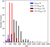 |
Fig. 1 Histogram presenting both the H magnitude and the S/N (from APOGEE) of our M dwarf sample stars. |
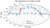 |
Fig. 2 Map showing the location in the sky of our sample M dwarfs. Kepler target field is highlighted in red. |
2.2 Sample characterization
We display both the magnitude distribution and the APOGEE-estimated S/N of our 313 sample stars in Fig. 1. The figure shows how most of our sample has high S/N spectra and also shows how fainter stars tend to have lower S/N, as expected. The small clump of lower-magnitude (4–6) S∕N < 300 stars corresponds to the M dwarfs from Souto et al. (2020) that were characterized using interferometry.
We display the location in the sky of all M dwarfs in the sample, showing both their right ascension (RA) and declination (Dec) in Fig. 2. Most of the stars are located in the northern hemisphere (Dec > 0 deg), as they were observed by APOGEE-2N. Nineteen stars in our sample are located in the Kepler field (Latham et al. 2005), fourteen of which have been observed by the Kepler Space Telescope.
2.3 Available literature values for the sample
We cross-matched our M dwarf sample with different surveys and works related to spectroscopic stellar characterization. We found eight works with stars in common with our sample that serve as our literature comparisons – ASPCAP (Garcia Pérez et al. 2016), Terrien et al. (2015), Gaidos et al. (2014), Hejazi et al. (2020), Souto et al. (2020), Passegger et al. (2019), Rajpurohit et al. (2018a,b). This subsection is dedicated to a discussion of these works and their determined parameters for the stars in common between them and our M dwarf sample.
 |
Fig. 3 ASPCAP Teff and [M/H] values for M dwarfs in sample, with overplotted PARSEC isochrones (Bressan et al. 2012) for an age of 5 Gyr created with different log g values (scale is in dex). Points are color coded based on the metallicity value derived for each star. |
2.3.1 ASPCAP
The ASPCAP (Garcia Pérez et al. 2016) is the pipeline dedicated to the derivation of spectroscopic parameters for stars observed with APOGEE, with estimates published for stars in our sample as well. The ASPCAP pipeline provides both a preliminary set of output parameters for each observed star as well as a final set of calibrated parameters focused on its main target of giant stars. However, their calibrated parameter ranges do not include all M dwarfs in our sample, as their lower boundary for Teff is 3200 K. Their values can still serve as an important reference for our pipeline, as they have been shown to be consistent by Schmidt et al. (2016), who performed an extensive analysis on both the Teff and [M/H] values that ASPCAP produced for 3834 M dwarfs, comparing them to photometric and interferometric parameters for the same stars. Based on interferometric data from Boyajian et al. (2013), color-Teff relations from Mann et al. (2015), and the infrared flux technique published by Casagrande et al. (2008), they concluded that the ASPCAP Teff is accurate to about 100 K for stars between 3550–4200 K, and [M/H] values are accurate to about 0.18 dex. This means that despite the main focus of ASPCAP on giant stars – and not M dwarfs – we can take their measurements of Teff and [M/H] as consistent for the parameters of M dwarfs in our sample and we will thus use them as a comparison value for our analysis.
From the 313 stars in our sample, ASPCAP published their final, calibrated [M/H], Teff, and log g for 283 stars. These values are displayed in Fig. 3, with the color indicating the ASPCAP log g values for each star. The figures shows that their Teff values are concentrated around 3600–3800 K, and [M/H] are between −0.4 and +0.0 dex. The metallicity distribution follows an approximate Gaussian shape, with an average value of −0.29 dex and a standard deviation of 0.27 dex. These results show that a significant fraction of stars in our sample are early M dwarfs. According to ASPCAP results, our sample is, on average, more metal-poor than the solar neighborhood, which has mean metallicity values around −0.20 dex (Holmberg et al. 2007).
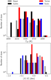 |
Fig. 4 Teff (top) and [M/H] (bottom) values from four literature sources: Gaidos et al. (2014) (black, Teff for 40 stars, [Fe/H] for 24 stars), Hejazi et al. (2020) (orange, filled bars, 19 stars), Terrien et al. (2015) (red, 45 stars), and an aggregate of Souto et al. (2017), Souto et al. (2018), and Souto et al. (2020) (blue, 24 stars). The number of stars is displayed with logarithmic notation for visibility. |
2.3.2 Terrien et al. (2015)
From the 886 stars characterized in Terrien et al. (2015), 45 are included in our sample. Their spectra have wide coverage (0.8−2.4 μm) but low resolution (R ~ 2000). Their Teff values are determined by analysis of water indices in the K band and have uncertainties above 100 K, and their [M/H] values are measured using empirical spectroscopical calibrations with uncertainties around 0.12 dex. Their published parameters are shown in Fig. 4. Comparing their parameter distribution with the full ASPCAP sample, we find that Terrien et al. (2015) is more representative of later-type M dwarfs, having a significant fraction of stars with published Teff between 3200 and 3500 K.
2.3.3 Souto et al. (2017, 2018, 2020)
We find that some of the best characterized stars in the APOGEE sample are the M dwarfs that were analyzed bySouto et al. (2017, 2018, 2020). That is because these works use spectral synthesis and a combination of MARCS and PHOENIX model atmospheres to determine both stellar parameters and chemical abundances for eight different elements using APOGEE spectra. Their reported uncertainties are Teff ± 100 K, log g ± 0.2 dex and [Fe/H] ± 0.1 dex. A total of 24 different M dwarfs were characterized by this method – Kepler 138 and Kepler 186 in Souto et al. (2017), Ross 128 in Souto et al. (2018), and 21 other stars in Souto et al. (2020). Among all the stars in our sample previously characterized in the literature, the most metal-poor one is 2M03150093+0103083, with [Fe/H] = −0.91 dex, and it was characterized by Souto et al. (2020).
2.3.4 Gaidos et al. (2014)
Gaidos et al. (2014) analyzed optical spectra of nearby K and M dwarfs with R ~ 1000 and determined their spectroscopic parameters by fitting model spectra to observations. Their estimated errors vary between stars, but are around 100 K for Teff and 0.12 dex for [Fe/H]. From the 2970 stars with d < 50 pc observed by Gaidos et al. (2014), 28 are included in our sample and their parameters are shown in Fig. 4. The reduced number of stars, combined with the lack of [Fe/H] available for half the stars in the sample, does not allow for an extensive statistical analysis of this stellar subsample. Nevertheless, it is possible to note that Gaidos et al. (2014) reported Teff values between 3100–3500 K for a greater number of stars in this subsample than in the main ASPCAP one, helping us characterize the lower Teff stars in our sample. Gaidos et al. (2014) also found metallicity for stars in our sample across a larger parameter space (− 0.6 < [Fe/H] < +0.4 dex) than ASPCAP.
2.3.5 Hejazi et al. (2020)
Hejazi et al. (2020) published chemical properties for 1544 high proper-motion M dwarfs and subdwarfs from low-mid resolution (~ 2000−4000) optical spectra. A template-fit method was developed, based on the measurement of TiO and CaH molecular bands near 7000 Å. The analysis of 48 binary systems suggests precision levels of ± 0.22 for [M/H], ± 0.08 for [α∕Fe], and ± 0.16 for the combined index [M/H] + [α∕Fe]. We find 19 starsin common between our observed sample and their study. From Fig. 4, we can verify that the characterized stars are dispersed across a wide range of temperatures, with a stronger concentration of stars around Teff = 3600 K. As for the metallicities, we find stars both above and below solar neighborhood values, but no star within − 0.1 < [M/H] < +0.1 dex, which must be considered when comparing our results to theirs.
2.3.6 Passegger et al. (2019)
We cross-matched our sample with the 300 stars characterized by Passegger et al. (2019) and found 14 stars in common. As mentioned in Sect. 1, this work derived parameters for M dwarfs by using a χ2 to fit PHOENIX-SESAM models to high-resolution (R ~ 90 000) CARMENES spectra in both the visible and infrared wavelength ranges. Their reported uncertainties depend on each star’s rotational velocity and, for NIR spectra, are as low as 51 K for Teff, 0.07 for log g, and 0.16 for [Fe/H].
2.3.7 Rajpurohit et al. (2018a)
Another study based on CARMENES spectra is Rajpurohit et al. (2018a). This work focused on matching BT-Settl model spectra to CARMENES optical and NIR observations of 292 M dwarf spectra. Since this work determines parameters by matching observed spectra to a grid of previously computed models, the reported uncertainties correspond to the size of the grid, 100 K for Teff and 0.1 dex for both log g and [M/H]. We find 12 stars in common between our sample and the one characterized by Rajpurohit et al. (2018a), which are part of the 14 stars later characterized by Passegger et al. (2019) and listed in Sect. 2.3.6.
2.3.8 Rajpurohit et al. (2018b)
The same technique was applied to 45 M dwarfs observed with APOGEE in Rajpurohit et al. (2018b). We have eight stars in common, with six of them having Teff < 3300 K, and are some of the coldest stars in our sample. The reported uncertainties for the parameters of these stars are Teff ± 100 K, log g ± 0.3−0.5 dex and [M/H] ± 0.05 dex. A comparison between our derived parameters and the previously available parameters for these stars is available in Fig.13.
We found López-Valdivia et al. (2019) as an example of another large-scale, high-resolution study of spectroscopical parameters for M dwarfs in the infrared, but, unfortunately, it shares no stars in common with APOGEE. The best spectroscopic parameters available in literature for our sample stars are the ones cited in this section and ASPCAP values. Therefore, comparisons between our results and literature values are made based on the works mentioned above.
3 Methodology
This section includes the steps in our method that are specific for M dwarfs. The full rundown of our pipeline is available at Sarmento et al. (2020). In summary, our first step is to normalize the APOGEE observed spectra for each star using the template method and a synthetic spectrum. Then we created custom software that uses iSpec (Blanco-Cuaresma et al. 2014; Blanco-Cuaresma 2019) and Turbospectrum (Alvarez & Plez 1998; Plez 2012) to derive the atmospheric parameters through a χ2 minimization algorithm that compares observed and synthetic spectra. These synthetic spectra are created using MARCS (Gustafsson et al. 2008) stellar atmospheric models and a custom line list. The best-fitting synthetic spectra are selected through χ2 minimization, using MPFIT (Markwardt 2009) internally through iSpec. Finally, the parameters of the best matching synthetic spectra are taken as our measurements for the stellar parameters of each star.
We created routines for the download, format conversion, normalization of the sample spectra, and we have made the pipeline as automated as possible, but the χ2 minimization and the synthesis of the best fitting spectra are done with Turbospectrum, controlled by iSpec python code. The custom routines are programmed in Python 3 and for the 2020 distribution of iSpec. They are included in a public repository together with the full results, line lists, line masks, and everything required to replicate the process described in this paper1.
3.1 Line list
The line list used for M dwarf spectral syntheses is more complex than the one used for the spectra of FGK stars, as these stars have many water (H2O) lines that are not visible in hotter stars. These water lines form a thick blanket that makes the flux continuum harder to identify, as shown in Fig. 5. We use the water line list first published in Barber et al. (2006), retrieved from Bertrand Plez’s personal website2. We note that a more recent work on water lines was published by Polyansky et al. (2018), but preference was given to usage of the water line list from Barber et al. (2006) as it was already formatted for Turbospectrum and of a more computationally manageable size. A total of 1 263 825 water lines were included in the M dwarf line list, along with the 85 334 lines from other molecules and atoms already available at Sarmento et al. (2020), made from a combination of the Vienna Atomic Line Database (VALD, Piskunov et al. 1995) and the APOGEE line list (Shetrone et al. 2015). This resulted in a final list of 1 349 159 lines.
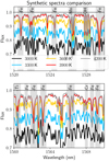 |
Fig. 5 Comparison between synthetic spectra made with different Teff. The spectra corresponds to synthesis made with Teff 4200 K (gray), 3900 K (red), 3600 K (orange), 3300 K (orange) and 3000 K (black). |
3.2 Normalization of the spectra
As we can see in Fig. 5, a 300 K difference in Teff can mean a 0.05 difference in the continuum flux for a star, which is enough to turn an accurate fit into a terrible one. Therefore, in order to accurately normalize an M dwarf’s H-band spectrum, an accurate initial input stellar Teff for that star is required. Normalizations with templates synthesized with Teff closer to the star’s real Teff will result in continuum values closer to the real ones, meaning the synthetic spectra will closely resemble the observed ones. Therefore, the first important step towards deriving a star’s atmospheric parameters is to have good estimates for their Teff and metallicity.
Given the lack of a consistent literature source for the Teff of our sample stars and in order to minimize the effect of the visual choice of Teff based on the normalized spectra, the spectrum of each star in our sample was normalized using synthetic spectra with 148 different combinations of Teff, log g and [M/H], corresponding to values taken from PARSEC isochrones (Bressan et al. 2012) for stars with ages between 109 and 1010 yr. This approach is aimed at avoiding unrealistic combinations of output parameters. We selected isochrones with a 0.2 dex spacing in [M/H] values, rounding Teff values to the nearest multiple of 100 K, and log g being rounded to the nearest multiple of 0.1 dex. These values are selected to both have an amount of normalizations that can be computationally generated in a short amount of time and to have an even distribution across our expected parameter space for M dwarfs, as our sample stars are expected to have parameters approximating one of these combinations. The full list of parameter combinations is available at Appendix A.1.
Afterwards, we compared each of the normalized spectra to the template used to create the normalization. By calculating and minimizing the χ2 across our line mask region (see Sect. 3.3) between the observed and the template spectra, the parameters for the best normalization template are defined. Figure 6 displays the χ2 values for different normalization parameters for star 2M05201152+2457212. That figure shows how the χ2 values depend strongly on the normalization template and can indicate the quality of the template choice for normalization. It is also clear that templates with similar parameters have similar χ2 values. This fact shows that these values are close to the real stellar parameters, and the normalization with a template with Teff = 3700 K, log g = 4.7 dex, [M/H] = 0.0 dex can be used for this star in the next steps of the pipeline.
3.3 Line mask
As explained in Sarmento et al. (2020), a line mask instructs iSpec on which spectral regions should be considered for comparing observed and synthetic spectra. A line mask specifically made for M dwarf stars was therefore required for the code to match an appropriate model to the observations. The star Ross128 (2M11474440+0048164), as an APOGEE M-dwarf with S∕N ~ 229 previously characterized by Souto et al. (2018), was chosen as the basis for this line mask. A synthetic spectrum was generated using the parameters found for the star by Souto et al. (2018) (Teff = 3231 K, [Fe/H] = 0.03 dex and log g = 4.96 dex). This synthetic spectrum was used to normalize the observed one and then compare it. Regions and spectral lines with a good agreement between both spectra were selected for the line mask displayed in Fig. 7. The areas where the synthesis did not reproduce well the observed spectrum were discarded to create the final line mask shown. We note that despite the slight errors in the Al lines around 1675 nm, we included these lines in our line mask. This was done because the two Al lines are the strongest lines we find across our wavelength range, and they are very well reproduced across other stars (see, for example, Figs. B.2–B.4).
3.4 Free parameters
The free parameters used for the syntheses of M dwarf spectra are the same as the ones used in Sarmento et al. (2020) for the syntheses of the spectra of FGK stars – effective temperature (Teff), surface gravity (log g), metallicity ([M/H]), micro-turbulent velocity (vmic), projected rotational velocity (v sin i), and spectral resolution. The input values used are, for Teff, log g, and [M/H], the ones used tocreate the template spectra for the normalization (see Sect. 3.2). The initial values for the remaining free parameters are 1.06 km s−1 for the vmic, 1.6 km s−1 for v sin i, and 22 000 for the resolution. We note that despite leaving the resolution as a free parameter, our output values for this parameter are close to 22 000.
However, an important change required to keep the output parameters limited to realistic values is the restriction of possible output parameters to a given parameter space. Restricting the parameters to a given interval based on the starting values allows the code to both take the first guess given by the normalization template into account and, at the same time, allowing it to fine-tune the parameters towards optimal values for χ2 minimization. The output parameters are limited to the initial template parameters ± 350 K (for Teff), ± 0.2 dex (log g) and ± 0.3 dex ([M/H]). We found these ranges through trial and error, and testing the method with multiple stars. Ultimately, they formulate a balance between the information given by the normalization template and the freedom required for the pipeline to find the best fit for a given spectrum.
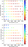 |
Fig. 6 Two scatter plots displaying the χ2 values measured for different spectroscopic parameter combinations for templates for the normalization of star 2M05201152+2457212. Top: Teff and metallicity; bottom: Teff and log g. |
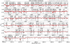 |
Fig. 7 Comparison between the observed spectrum of Ross 128 (2MASS J11474440+0048164), normalized using the template method (black), and a synthetic spectrum created using the literature (Souto et al. 2018) parameters for that star (red). The parameters used to generate the synthetic spectrum were Teff = 3231 K, log g =4.96 dex, [M/H] = +0.03 dex. The ASPCAP preliminary parameters for this star are Teff = 3212 K, log g =4.45 dex, [M/H] = −0.60 dex. The areas in gray represent the ones included in the line mask created from these spectra. |
3.5 Error estimation
Because of the way our pipeline is setup, we have two major possible error sources, one associated with a poor choice of normalization and one connected to Turbospectrum and the derivation of the best-fit synthetic spectrum for each star. In this section, we try to quantify the errors associated with both of these sources across our M dwarf parameter space.
3.5.1 Normalization template errors
As the shape of the characterized spectra, and the subsequently derived parameters, are strongly influenced by the normalization template used, we decided to test our pipeline by running multiple normalizations for the same observed star. A sample of four test stars was selected, covering a wide range of stellar parameters. For each test star, we ran the pipeline with all normalization templates with χ2 within a 10% margin from the best templates found for each star, using the χ2 values as an indication that the template is appropriate for the studied star. We ran the pipeline 20 times for each normalization template, injecting Gaussian errors proportional to the S∕N. The errors are injected in such a way that the deterministic pipeline does not return the same output parameters on every iteration, allowing us to understand how the parameters can change across multiple observations of the same star. We do note here that these tests result in an underestimation of the actual errors, as errors affecting the continuum normalization will produce correlations across multiple pixels. Therefore these serve as a minimum estimate for the actual errors in our measurements. Table 1 summarizes our results for a test sample of 4 stars, including the average and standard deviation obtained across the 20 runs of the pipeline for each normalization template per star.
The results displayed demonstrate that the output parameters can vary significantly with the template used for the normalization of the spectra. They also demonstrate the difficulty in assessing which template works best for a given star, as χ2 values can be very similar even for spectra with varying parameters. The standard deviation verified within the same template used also shows the consistency of the pipeline itself for a given spectrum, which is further explored in the following section.
3.5.2 Errors associated with S/N
In order to estimate the errors associated with the S/N inherent to the spectra and the method used to find the best fit for each normalized spectra, a sample of 20 M dwarfs with different S/N and stellar parameters was selected. The pipeline was ran 20 times per star, with Gaussian errors proportional to the reported S/N of each star injected into the observed spectra before normalizing them with the method described in Sect. 3.2 Similar to the tests described in Sect. 3.5.1, these are also underestimations of the possible errors, as only uncertainties associated with individual pixels are taken into account. In order to have a more statistically relevant sample size, 80 additional iterations of the pipeline were run for each of four selected stars that cover a wide parameter range, for a total of 100 pipeline iterations per star. The results of these tests are summarized in Table 2.
As shown in the table, the output of the pipeline is very consistent across multiple iterations, with Teff having standard deviations below 12 K, [M/H] < 0.03 dex and log g < 0.09 dex for all analyzed stars. There is no strong S∕N effect on the standard deviation measured, as the values remain very consistent across all stars in the sample. These tests suggest that most of the possible errors in the final results are a result of the templates used for the normalization of each observed spectrum, and showing that log g is the parameter with the largest associated error.
Given the errors measured in the displayed tests and the size of the grid used for the selection of the normalization template, we estimate the overall errors of our pipeline to be around Teff ± 100 K, [M/H] ± 0.1 dex and log g ± 0.2 dex, with a large percentage of these errors coming from the inherent uncertainty in the choice of normalization template used for a given star. This choice is limited by the PARSEC evolutionary code, as it is the only one publicly available covering the M dwarf parameter space with a good range coverage. Another possible error source can be the line mask used for the χ2 calculation, as χ2 values can be very similar for different normalization templates and changes in the line mask can result in the selection of different templates as well.
Average and standard deviation for stellar parameters measured for a sample of four stars, using different normalization templates and across 20 iterations of the pipeline for each star-normalization template combination.
3.6 Summary
This sectioncontains a small summary of the steps required to derive M dwarf stellar parameters using our pipeline.
144 different synthetic spectra are generated using parameter combinations taken from PARSEC isochrones and expected forM dwarfs. We note that the MARCS models in this parameter space are provided in steps of 100K for Teff, 0.25 dex for [Fe/H], and 0.5 dex for log g, and we interpolate between them to create the grid whenever necessary. This interpolation is done entirely within iSpec, and we have not edited that part of the code.
The observed combined spectrum for each sample star is downloaded from APOGEE and normalized using each of the previously generated synthetic template spectra.
The best normalization template for each star is chosen, based on a χ2 comparison between each template and its resulting normalized spectrum.
iSpec (Blanco-Cuaresma et al. 2014; Blanco-Cuaresma 2019), as a shell for Turbospectrum (Alvarez & Plez 1998; Plez 2012), is used to generate synthetic spectra from a set of starting values. These synthetic spectra are created using MARCS (Gustafsson et al. 2008) stellar atmospheric models and a custom line list.
Specific line masks are required for the synthesis of spectrum of stars with different spectral types and these include the most relevant wavelength areas for spectral parameter determinations.
The synthetic spectra are matched to the normalized observed ones through a χ2 minimization algorithm based on MPFIT (Markwardt 2009). The algorithm runs on a list of previously selected wavelength regions defined as the line mask.
χ2 minimization is used to find the best match between a synthetic spectrum and a given observed one, interpolating the available MARCS whenever necessary. Then the spectral parameters used to generate the synthetic spectrum are taken as corresponding to the observed star.
4 Results
The spectra of the 313 M dwarfs in our sample were analyzed on the basis of the method detailed in Sect. 3, with the derived Teff, log g and [M/H] plotted in Figs. 8 and 9. The full results are available online for download at CDS. The errors included in the plots are ±100 K for the Teff, log g ± 0.2 dex, and [M/H] ± 0.1 dex. Figure 10 includes the parameters derived with APOGEE DR14 and the full list of parameters derived with that Data Release is included in Table D.1.
The isochrone comparisons presented in Fig. 8 show that, as expected, for most of the sample, our methodology’s output Teff and log g agree with the values predicted by the PARSEC models for M dwarfs. Despite this, the output log g values for a small number of stars is either overestimated or underestimated when compared to isochrone predictions. Some weak trends are also present across the results for the full sample in Fig. 9, with thin columns of stars with very similar effective temperatures but different metallicity values. We do not know exactly what causes these trends. We find these values to cluster around multiples of 100 K, and MARCS models have spacings of 100 K for 2500 K < Teff < 4000 K (compared with 250 K for 4000 K < Teff < 8000 K), but further tests with the interpolation of the models have not shown any issues.
The lower limit of our analysis is around Teff = 3000 K. From the sample of stars with ASPCAP Teff < 3000 K, we found the normalization template with the lowest χ2 for three of them to converge to synthetic spectra with very high metallicity values ([M/H] = 0.4 dex). For the full results derived for these stars, see Table 3. This result corresponds to the highest possible [M/H] using our normalization method and to the limit of the MARCS models used to generate synthetic spectra. The output parameters for these three stars are very similar among them and are outside the expected values for M dwarfs. We do not think these output parameters represent a reliable measurement for these stars and they are included here only as a demonstration of the limitations of our method for stars with Teff< 3000 K. We think that the limitations of our pipeline are caused by our optimization of the line list to reproduce the spectra of stars with higher Teff, missing possible opacity sources for lower temperature stars and the pipeline compensating these deficiencies by decreasing the Teff and increasing the [M/H] of the synthetic spectra. These effects increase the strength of the water lines present in the spectrum, but the resulting parameters will not be reliable.
We find the spectra of stars with 3000 < Teff < 3500 K to be especially challenging to reproduce synthetically given the degeneracy in the continuum absorption among multiple spectral parameters, such as temperature, metallicity, and surface gravity. Absorptions in the continuum can be caused by any of these parameters, with the pipeline sometimes estimating lower metallicity and higher temperature values than the realistic values characterizing the star.
We present an example of synthesized stellar spectra for a star with Teff ~ 3500 K in Fig. 11. Here, the spectra of star 2M18244689-0620311 (BD-06 4756B3) is displayed,showing both the observed (black) and best matching spectra (red). This star was characterized in Souto et al. (2020) as having Teff = 3376 K, log g = 4.77 dex, [M/H] = +0.21 dex. The available ASPCAP parameters for this star are Teff = 3502 K, log g = 4.63 dex, and [M/H] = −0.17 dex. The displayed spectrum for the star has been obtained by normalizing the APOGEE observed one with a synthetic spectrum with Teff = 3500 K, log g = 4.9 dex and [M/H] = −0.2 dex, and the derived spectroscopical parameters for this star are Teff = 3484 ± 100 K, log g = 4.85 ± 0.2 dex, [M/H] = −0.15 ± 0.1 dex.
The presence of a wide water line band is noticeable across the full spectrum, especially the full first order (two top rows), resulting in a jagged and depressed continuum down to around 0.9 instead of the expected 1.0. The modeling of these water lines is fundamental for the creation of an accurate synthetic spectra of late M dwarfs (Teff < 3500 K). This star is slightly below solar metallicity, still retaining pronounced molecular and elemental lines. The effect can be noticed in the strong Al line around 1675 nm, a line that is accurately matched by the synthetic spectrum. The synthesized spectrum matches the observed one across the full wavelength range, with lines of multiple elements and molecules being correctly synthesized. This fact, combined with the relative agreement of our pipeline’s derived parameter with available literature analysis, increases our confidence in the derived parameters for this star.
Additional examples of output spectra obtained by our pipeline are displayed in Figs. B.2–B.5, with more stars across our parameter space.
Average and standard deviation for stellar parameters measured for multiple iterations for 20 selected stars representative of the full sample.
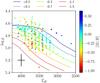 |
Fig. 8 HR diagram with Teff and log g values from iSpec output parameter distribution, with overplotted PARSEC isochrones (Bressan et al. 2012) for an age of 5 Gyr created with different [M/H] values (scale is in dex). Points are color-coded based on the metallicity value derived for each star. Plotted parameters were obtained with APOGEE DR16. |
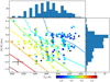 |
Fig. 9 Teff and [M/H] from iSpec parameter distribution for stars in M dwarf sample, with overplotted PARSEC isochrones (Bressan et al. 2012) for an age of 5 Gyr created with different log g values (scaleis in dex). Points are color-coded based on the surface gravity value derived for each star. Plotted parameters were obtained with APOGEE DR16. |
Output parameters for 6 stars with Teff ≤ 3000 K.
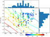 |
Fig. 10 Teff and [M/H] from iSpec parameter distribution for stars in M dwarf sample, with overplotted PARSEC isochrones (Bressan et al. 2012) for an age of 5 Gyr created with different log g values (scale is in dex). Points are color coded based on the surface gravity value derived for each star. The plotted parameters were obtained with APOGEE DR14. |
5 Analysis
5.1 ASPCAP comparison
As mentioned in Sect. 2.3, there are no available final ASPCAP spectroscopic parameters for all stars in our sample. From the full 313 star sample, we have ASPCAP calibrated values for Teff, [M/H], and log g for 283 of them. Therefore, all comparisons shown and discussed here will focus on those 283 stars. We do not show raw or spectroscopic parameters for reasons of consistency. Figure 12a shows a comparison between the Teff values for our sample M dwarfs as derived by our pipeline and the calibrated values published by ASPCAP for the same stars, (b) presents the same comparison for ASPCAP calibrated [M/H] values, and (c) shows a comparison between the log g values derived with our pipeline and the calibrated ones published by ASPCAP. The errors that are included are estimated based on our normalization grids and are ±100 K for the Teff, ± 0.1 dex for [M/H] and ± 0.2 dex for log g (see Sect. 3.5). The points are colored according to other parameters measured by our method in order to highlight any correlation or trend between errors across multiple output parameters.
In Fig. 12a, and relative to ΔTeff, we find a small trend of more negative ΔTeff for stars with Teff < 3500 K. For stars above this Teff, we find verysimilar values between our analysis and the parameters published by ASPCAP. Additionally, we find no correlation between ΔTeff and each star’s metallicity values. Overall, we find this parameter to be in good agreement with ASPCAP published results, with the median difference as well as the SD and MAD all being within our error margins.
As for Fig. 12b and [M/H], a trend is present here, as we find a negative Δ[M/H] for the stars in our sample with Teff > 3400 K and a positive one for stars with Teff < 3400 K. This translates to an overestimation of metallicity for the colder stars in our sample when compared to ASPCAP values. Both lower Teff and increasing [M/H] can have a similar effect on the spectral shape, lowering the continuum position due to an increased strength of the water molecular lines. Therefore, metallicity overestimations can be caused by normalization errors or may correspond to effective temperature underestimations. We must note that here we are using the Teff values determined by our pipeline to color the points.
For log g, Fig. 12c shows that a small trend is present in the data, with negative Δ log g values for stars with lower log g. The overall distribution is not very different, with median differences of +0.07 dex between our parameters and the ones published by ASPCAP, although with SD and MAD around our uncertainty levels. We find a wide range of differences in log g, with the comparisons varying between −0.6 dex and +0.4 dex. Comparisons with the isochrones in Fig. 8 show that our values for this parameter are within the expectations for main-sequence stars around these temperatures. A direct comparison between Figs. 3, 9, and 10 shows how the ASPCAP calibrated log g values differ from our derived parameters for our M dwarf sample. While our values using data from DR16 follow the isochrones approximately, both the results with DR14 and their parameters seem to vary wildly, especially for M dwarfs with Teff < 3800 K/ log g > 4.9 dex. This does appear to indicate that our method provides more plausible surface gravity values given our current stellar modeling knowledge, as reflected in the overplotted PARSEC isochrones. It also shows how the spectra provided by APOGEE had improved between DR14 and DR16, lending credence to the notion that the more recent data release is of higher quality than the previous one.
Overall, we find that the best agreement between our parameters and the ones published by ASPCAP is found for [M/H], despite some trends being present alongside Teff and log g. All of these comparisons were made with calibrated ASPCAP parameters, which should not be ignored, as they can show inherent bias in the method and the output parameters.
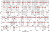 |
Fig. 11 Comparison between APOGEE spectra of the star 2M18244689-0620311 (black, normalized using a synthetic spectra with Teff = 3500 K, log g =4.9 dex and [M/H] = −0.2 dex) and the best-fitting synthetic spectra (red, straight line) for APOGEE wavelength range. In gray, we highlight the areas used for χ2 minimization by our pipeline algorithm. The best fitting parameters derived were Teff = 3507 ± 100 K, log g =4.80 ± 0.2 dex, [M/H] = −0.19 ± 0.1 dex. The available ASPCAP parameters are Teff = 3600 ± 59 K, log g =5.09 ± 0.12 dex, and [M/H] = −0.06 ± 0.01 dex. This star was characterized in Souto et al. (2020) as having Teff = 3376 K, log g =4.77 dex, [M/H] = +0.21 dex. |
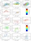 |
Fig. 12 Comparisons between our output parameters and those available in the literature, colored according to either our method’s measured [M/H] (Teff plots, left column; see scale at (f)) or Teff for each star ([M/H], center column, and log g, right column, see color scale at (l)). From top to bottom: comparisons with ASPCAP (a, b, c), Terrien et al. (2015) (d, e), Souto et al. (2020) (g, h, i), Gaidos et al. (2014) (j, k), Hejazi et al. (2020) (m, n, o). Temperature values are displayed in Kelvin, while metallicity and surface gravity are in dex. |
Median differences between our results and literature parameters.
5.2 Other literature comparisons
5.2.1 Comparison with Terrien et al. (2015)
Figures 12d,e show a comparison between the parameters derived with our pipeline and the ones published in Terrien et al. (2015) for 45 stars in common between both samples. Table 4 shows the median difference, standard deviation and mean absolute deviation found when comparing both distributions. As Terrien et al. (2015) does not publish values for log g, we kept thespace reserved for the plot for that parameter (right column) empty. We find the differences between them to be above the uncertainty level, with the SD and MAD of the [M/H] values being slightly above (0.15 and 0.08 dexvs. 0.10 dex) and Teff slightly below (86 and 57 K vs. 100 K).
In the case of Teff, we find no large-scale trend or deviation between both parameter distributions, with ΔTeff < 250 K for all compared stars and with no correlation with [M/H]. However, the fact that we find ΔTeff ≥ 0 K for almost the full sample, as well as a median difference of + 92 K, points towards small biases in either parameter distribution. As for Δ[M/H], it has a wider distribution, going up to ±0.3 dex, and a median difference of − 0.19 dex can point towards systematic trends in our output data. There is also a linear trend towards negative Δ[M/H] for stars with [M/H] < −0.2 dex and Teff ~ 3300 K.
5.2.2 Comparison with Souto’s parameters
Figures 12g–i show a comparison between the parameters derived by our pipeline and the ones published in Souto et al. (2017, 2018, 2020) for 24 M dwarfs. We should note that as Souto et al. published [Fe/H] for their characterized stars and our method measures [M/H], that discrepancy can explain some of the differences. The differences between results published by both methods are also summarized in Table 4.
We find clear differences between both parameter distributions, with lower metallicity values (Δ[M/H] = −0.23 dex) and higher temperatures (ΔTeff = +109 K) for our stars. These trends fall in line with the results for the previously compared Terrien et al. (2015) results, with negative Δ[M/H] and positive ΔTeff, with the metallicity differences being above our uncertainty levels. Like the previous comparison, we find no cross-parameter trends, as the [M/H] differences seem to be independent of Teff and vice versa. We also find a weak linear trend with log g itself, as we find lower Δlog g for stars with log g < 4.8 dex, and a higher Δlog g for stars with log g > 4.8 dex (with a correlation coefficient of ρ = 0.71).
5.2.3 Comparison with Gaidos et al. (2014)
We present, in Fig. 12j, a comparison between our Teff results and the ones published in Gaidos et al. (2014) for 40 stars in common between both samples. Figure 12 k shows a similar comparison for [M/H] for the 24 stars with that parameter in the common sample. Similar to the case of Terrien et al. (2015), we have no reference value for log g from this source, so the space for the plot for that parameter (right column) is kept empty. Additionally, Table 4 presents themedian, standard deviation and mean absolute deviation found when comparing both parameter distributions.
Similar to the previous comparisons, we find trends towards both positive ΔTeff and negative Δ[M/H]. We find the standard (91 K) and mean absolute deviations (81 K) to be slightly around our estimated uncertainties for temperature, while the median differences (+56 K) are below them. As for metallicity, they are slightly above our uncertainty levels. There is a small trend towards lower Δ[M/H] for colder objects, but since the number of stars is so small, it might turn out to be a statistical artifact.
5.2.4 Comparison with Hejazi et al. (2020)
We present,in Figs. 12m–o, a comparison between our output values and the ones published in Hejazi et al. (2020) for 19 stars in common between both samples. Additionally, Table 4 presents the differences between results obtained by both methods. We find positive ΔTeff, with standard (81K) and mean absolute (78 K) deviations around our estimated uncertainties for the parameter. We also find strong trends in both log g and [M/H] distributions, with deviations significantly above our estimated uncertainty values.
As for discrepancies in Teff, Fig. 12m shows that the ΔTeff distribution between both methods is not very large, with most stars having a ΔTeff ~ ±120 K. The strongest outlier is star 2M07404603+3758253, which we find to have Teff = 3325 K and [M/H] = −0.62 dex, while Hejazi et al. (2020) published Teff = 3200 K and [M/H] = +0.4 dex for the same star4.
A [M/H] comparison shows a linear trend in Fig. 12n, with Δ[M/H] ~ −1.0 dex for metal-poor stars, and Δ[M/H] ~ 0.0 dex for stars around solar metallicity. We also find significantly lower values for metallicity than Hejazi et al. (2020), with an average Δ[M/H] = −0.43 dex. Despite their reported uncertainties of ±0.22 dex, this is a significant difference. Similarly to the comparison with Gaidos et al. (2014) (Fig. 12k), and unlike the ASPCAP comparison (Fig. 12b), there is a trend towards lower Δ[M/H] for colder objects. Some possible explanations can be the lower resolution of their analysis and the fact that it was done in the optical (not in the NIR) but the fact that the trends are very similar across all literature comparisons presented here leads us to believe in the presence of an inherent bias in our pipeline towards low [M/H] output parameters.
For log g, we find a linear trend towards measuring lower Δlog g for stars with log g < 4.9 dex, and a higher Δlog g for stars with log g > 4.9 dex. This is very similar to the Δlog g plot for our Souto values comparison (see Fig.12i) and can point towards some issues with the log g determined by our method.
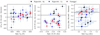 |
Fig. 13 Comparison in derived parameters between our method and the 8 stars in common with Rajpurohit et al. (2018b; APOGEE) and the 12 stars in common with Rajpurohit et al. (2018a; CARMENES), and the 14 with Passegger et al. (2019; difference between our pipeline and literature). |
5.2.5 Comparison with Rajpurohit et al. (2018b)
We display a comparison between our output parameters and the results published by Rajpurohit et al. (2018b) for 8 stars in common in Fig. 13. Due to the low number of stars compared, no real statistical analysis can be made from this comparison. We find some small differences in the results across the stellar sample, with the clearest example being star 2M06320207+3431132, with an output Teff = 3465 K (our results) versus 3200 K. Similarly to the previous comparisons, we find a generally positive (but close to our uncertainty levels) value for ΔTeff. Unlike the previous results, we actually find a positive Δ[M/H] as well, while the largest difference between our results and theirs is in surface gravity, with some stars having Δ log g ~ −0.6 dex.
5.2.6 Comparison with Rajpurohit et al. (2018a) and Passegger et al. (2019)
As our sample and those of both Rajpurohit et al. (2018a) and Passegger et al. (2019) have only 12 stars and 14 stars in common, respectively,we compared our results with the parameters for each of them in Fig. 13. No overall trends are present in Teff, with the exception of a single star, 2M11474440+0048164, for which Rajpurohit et al. (2018a) gives Teff= 3500 K, whereas our analysis output is Teff = 3202 K. This star, however is characterized in Passegger et al. (2019) as having Teff= 3267 K, and by Souto et al. (2018) as having Teff = 3231 K. Both these literature values are much closer to our results, indicating the results of Rajpurohit et al. (2018a) to be an outlier. As for metallicity, we find Δ[M/H] ~ − 0.3 dex, in line with other literature comparisons, and we keep in mind that the comparison with Passegger et al. (2019) is based on their values for [Fe/H] rather than [M/H]. As for log g, we find our output parameters to be very similar to the ones published by Passegger et al. (2019), but some differences are present in the comparison with Rajpurohit et al. (2018a), with our values being up to 0.8 dex below theirs for three stars in common. However, similarly to the Teff for star 2M11474440+0048164, the log g values published by Passegger et al. (2019) for these stars are also much closer to our measurements, with a Δ log g ~ 0.05 dex.
6 Conclusions
Building on the method previously presented in Sarmento et al. (2020), we derived stellar atmospheric parameters for 313 M dwarfs with 3000 K < Teff ± 100 K < 4200 K, 4.5 dex < log g ± 0.2 dex < 5.3 dex and − 1.05 dex < [M/H] ± 0.1 dex < 0.56 dex. The pipeline uses iSpec as a spectroscopic framework to control Turbospectrum code and requires both a complete line list at the studied wavelength and a line mask tailored for the spectral type of the analyzed stars. We include both of these resources with this paper, along with all the derived stellar parameters, for future reference.
Our series of literature comparisons demonstrates the difficulty in finding accurate parameters for M dwarfs. Positive ΔTeff values are found across multiple literature comparisons, except for the ASPCAP values, although these are usually within the uncertainty levels. However, the additional presence of negative Δ[M/H] values in most of our literature comparisons suggest the existence of issues with the temperature and metallicity determination in our pipeline, as the effects of changes in these parameters in the M dwarf regime are not independent. We also note that our results are also dependent on the assumptions of the PARSEC evolutionary code. More analysis needs to be done on this subject.
Despite the existence of these trends, the strong match between synthesized and observed spectra for a wide range of M dwarf stars shows the power of the pipeline as a method for parameter determination. Future works could apply the method to NIR spectra observed with other instruments with a better resolution than APOGEE, such as CARMENES (R = 80 000−100 000, Quirrenbach et al. 2014), GIANO (R ~ 50 000, Origlia et al. 2014), SPIROU (R ~ 75 000, Artigau et al. 2014), NIRPS (R ~ 90 000−100 000 Wildi et al. 2017), and CRIRES+ (R ~ 100 000, Dorn et al. 2014). Expanding the characterized parameter space thanks to an analysis of a larger M dwarf sample and shifting to more complete and detailed molecular line lists are other ways that the performance of our method could be improved upon.
Acknowledgements
This work was supported by FCT – Fundação para a Ciência e a Tecnologia through national funds (PTDC/FIS-AST/28953/2017, PTDC/FIS-AST/7073/2014, PTDC/FIS-AST/32113/2017, UID/FIS/04434/2013) and by FEDER – Fundo Europeu de Desenvolvimento Regional through COMPETE2020 – Programa Operacional Competitividade e Internacionalização (POCI-01-0145-FEDER-028953, POCI-01-0145-FEDER-016880, POCI-01-0145-FEDER-032113, POCI-01-0145-FEDER-007672). This work was supported by Fundação para a Ciência e a Tecnologia (FCT) through the research grants UID/FIS/04434/2019, UIDB/04434/2020 and UIDP/04434/2020. This research has made use of NASA’s Astrophysics Data System. P.S. acknowledges the support by the Bolsa de Investigação PD/BD/128050/2016. E.D.M. acknowledges the support by the Investigador FCT contract IF/00849/2015/CP1273/CT0003 and in the form of an exploratory project withthe same reference. B.R.A. acknowledges funding support from FONDECYT through grant 11181295.
Appendix A Parameter combination list for the normalization
Parameter combination list used for the template normalization.
Appendix B More example synthetic and observed spectra comparisons
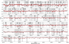 |
Fig. B.1 Comparison between APOGEE spectra of the star 2M03190939+0130543 (black, normalized using a synthetic spectra with Teff = 3200 K, log g =5.1 dex and [M/H] = −0.4 dex) and the best-fitting synthetic spectra (red, straight line) for APOGEE wavelength range. In gray, we highlight the areas used for χ2 minimization by our pipeline algorithm. The best-fitting parameters derived are: Teff = 3199 ± 100 K, log g = 5.1 ± 0.2 dex, [M/H] = −0.37 ± 0.1 dex. The available ASPCAP parameters are Teff = 3287 ± 60 K, log g =5.17 ± 0.14 dex and [M/H] = −0.57 ± 0.02 dex. |
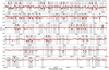 |
Fig. B.2 Comparison between the APOGEE spectra of the star 2M08050361+4121251 (G 111-52, black, normalized using a synthetic spectra with Teff = 3400 K, log g =5.0 dex and [M/H] = −0.6 dex) and the best fitting synthetic spectra (red, straight line) for APOGEE wavelength range. In gray, we highlight the areas used for the χ2 minimization by our pipeline algorithm. The best-fitting parameters derived are: Teff = 3413 ± 100 K, log g =4.98 ± 0.2 dex, [M/H] = −0.78 ± 0.1 dex. |
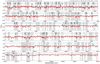 |
Fig. B.3 Comparison between the APOGEE spectra of the star 2M18562628+4622532 (black, normalized using a synthetic spectra with Teff = 3200 K, log g =5.0 dex and [M/H] = −0.2 dex) and the best fitting synthetic spectra (red, straight line) for APOGEE wavelength range. In gray, we highlight the areas used for the χ2 minimization by our pipeline algorithm. The best-fitting parameters derived are: Teff = 3204 ± 100 K, log g =4.99 ± 0.2 dex, [M/H] = −0.19 ± 0.1 dex. The available ASPCAP parameters are Teff = 3430 ± 58 K, log g =5.09 ± 0.13 dex and [M/H] = −0.44 ± 0.02 dex. |
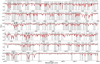 |
Fig. B.4 Comparison between the APOGEE spectra of the star 2M02073745+1354497 (black, normalized using a synthetic spectra with Teff = 3800 K, log g =4.7 dex and [M/H] = +0.0 dex) and the best-fitting synthetic spectra (red, straight line) for APOGEE wavelength range. In gray, we highlight the areas used for χ2 minimization by our pipeline algorithm. The best-fitting parameters derived were Teff = 3819 ± 100 K, log g =4.69 ± 0.2 dex, [M/H] = +0.01 ± 0.1 dex. The available ASPCAP parameters are Teff = 3866 ± 63 K, log g =4.83 ± 0.11 dex and [M/H] = +0.11 ± 0.01 dex. |
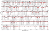 |
Fig. B.5 Comparison between the APOGEE spectra of the star 2M23460112+7456172 (black, normalized using a synthetic spectra with Teff = 3600 K, log g =5.0 dex and [M/H] = −0.6 dex) and the best-fitting synthetic spectra (red, straight line) for APOGEE wavelength range. In gray, we highlight the areas used for the χ2 minimization by our pipeline algorithm. The best-fitting parameters derived are: Teff = 3588 ± 100 K, log g =5.13 ± 0.2 dex, [M/H] = −0.49 ± 0.1 dex. The available ASPCAP parameters are Teff = 3560 ± 62 K, log g =4.86 ± 0.13 dex and [M/H] = −0.44 ± 0.02 dex. |
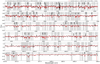 |
Fig. B.6 Comparison between the APOGEE spectra of the star 2M07404603+3758253 (black, normalized using a synthetic spectra with Teff = 3300 K, log g =5.0 dex and [M/H] = −0.4 dex) and the best-fitting synthetic spectra (red, straight line) for the APOGEE wavelength range. In gray, we highlight the areas used for the χ2 minimization by our pipeline algorithm. The best-fitting parameters derived are: Teff = 3325 ± 100 K, log g =4.97 ± 0.2 dex, [M/H] = −0.60 ± 0.1 dex. |
Appendix C Full results for stellar sample, DR16
The table C.1 is available online at the CDS.
Appendix D Full results for stellar sample, DR14
All derived parameters for the stellar sample from APOGEE DR14.
References
- Ahumada, R., Allende Prieto, C., Almeida, A., et al. 2020, ApJS, 249, 3 [CrossRef] [Google Scholar]
- Alonso-Floriano, F., Morales, J., Caballero, J., et al. 2015, A&A, 577, A128 [NASA ADS] [CrossRef] [EDP Sciences] [Google Scholar]
- Alvarez, R., & Plez, B. 1998, A&A, 330, 1109 [NASA ADS] [Google Scholar]
- Artigau, É., Kouach, D., Donati, J.-F., et al. 2014, Int. Soc. Opt. Photon., 9147, 914715 [Google Scholar]
- Barber, R., Tennyson, J., Harris, G. J., & Tolchenov, R. 2006, MNRAS, 368, 1087 [NASA ADS] [CrossRef] [Google Scholar]
- Blanco-Cuaresma, S. 2019, MNRAS, 486, 2075 [Google Scholar]
- Blanco-Cuaresma, S., Soubiran, C., Heiter, U., & Jofré, P. 2014, A&A, 569, A111 [NASA ADS] [CrossRef] [EDP Sciences] [Google Scholar]
- Bochanski, J. J., Munn, J. A., Hawley, S. L., et al. 2007, AJ, 134, 2418 [NASA ADS] [CrossRef] [Google Scholar]
- Bonfils, X., Delfosse, X., Udry, S., et al. 2013, A&A, 549, A109 [NASA ADS] [CrossRef] [EDP Sciences] [Google Scholar]
- Bowen, I., & Vaughan, A. 1973, Appl. Opt., 12, 1430 [NASA ADS] [CrossRef] [Google Scholar]
- Boyajian, T. S., von Braun, K., van Belle, G., et al. 2013, apj, 771, 40 [Google Scholar]
- Bressan, A., Marigo, P., Girardi, L., et al. 2012, MNRAS, 427, 127 [NASA ADS] [CrossRef] [Google Scholar]
- Casagrande, L., Flynn, C., & Bessell, M. 2008, MNRAS, 389, 585 [NASA ADS] [CrossRef] [MathSciNet] [Google Scholar]
- Delfosse, X., Forveille, T., Ségransan, D., et al. 2000, A&A, 364, 217 [NASA ADS] [Google Scholar]
- Deshpande, R., Blake, C., Bender, C., et al. 2013, AJ, 146, 156 [NASA ADS] [CrossRef] [EDP Sciences] [Google Scholar]
- Dorn, R. J., Anglada-Escude, G., Baade, D. a., et al. 2014, The Messenger, 156, 7 [Google Scholar]
- France, K., Froning, C. S., Linsky, J. L., et al. 2013, ApJ, 763, 149 [NASA ADS] [CrossRef] [Google Scholar]
- Gaidos, E., Mann, A., Lépine, S., et al. 2014, MNRAS, 443, 2561 [NASA ADS] [CrossRef] [Google Scholar]
- Garcia Pérez, A. E., Prieto, C. A., Holtzman, J. A., et al. 2016, AJ, 151, 144 [NASA ADS] [CrossRef] [Google Scholar]
- Gunn, J. E., Siegmund, W. A., Mannery, E. J., et al. 2006, AJ, 131, 2332 [Google Scholar]
- Gustafsson, B., Edvardsson, B., Eriksson, K., et al. 2008, A&A, 486, 951 [NASA ADS] [CrossRef] [EDP Sciences] [Google Scholar]
- Hejazi, N., Lepine, S., Homeier, D., Rich, R. M., & Shara, M. M. 2020, AJ, 159, 30 [Google Scholar]
- Henry, T. J., Jao, W.-C., Subasavage, J. P., et al. 2006, AJ, 132, 2360 [NASA ADS] [CrossRef] [Google Scholar]
- Holmberg, J., Nordström, B., & Andersen, J. 2007, A&A, 475, 519 [NASA ADS] [CrossRef] [EDP Sciences] [MathSciNet] [Google Scholar]
- Holtzman, J. A., Hasselquist, S., Shetrone, M., et al. 2018, AJ, 156, 125 [Google Scholar]
- Irwin, J. M., Berta-Thompson, Z. K., Charbonneau, D., et al. 2014, ArXiv preprint [arXiv:1409.0891] [Google Scholar]
- Jönsson, H., Holtzman, J. A., Allende Prieto, C., et al. 2020, AJ, 160, 120 [CrossRef] [Google Scholar]
- Latham, D., Brown, T., Monet, D., et al. 2005, Bull. Am. Astron. Soc., 37, 1340 [NASA ADS] [Google Scholar]
- Lépine, S., & Gaidos, E. 2011, AJ, 142, 138 [Google Scholar]
- Lépine, S., & Shara, M. M. 2005, AJ, 129, 1483 [Google Scholar]
- Lépine, S., Rich, R. M., & Shara, M. M. 2007, AJ, 669, 1235 [Google Scholar]
- López-Valdivia, R., Mace, G. N., Sokal, K. R., et al. 2019, ApJ 879, 105 [Google Scholar]
- Majewski, S. R., Schiavon, R. P., Frinchaboy, P. M., et al. 2017, AJ, 154, 94 [NASA ADS] [CrossRef] [Google Scholar]
- Mann, A. W., Brewer, J. M., Gaidos, E., Lépine, S., & Hilton, E. J. 2013, AJ, 145, 52 [NASA ADS] [CrossRef] [Google Scholar]
- Mann, A. W., Feiden, G. A., Gaidos, E., Boyajian, T., & von Braun, K. 2015, ApJ, 804, 64 [CrossRef] [Google Scholar]
- Markwardt, C. B. 2009, ASPC, 411, 251 [Google Scholar]
- Ness, M., Hogg, D. W., Rix, H.-W., et al. 2016, ApJ, 823, 114 [NASA ADS] [CrossRef] [Google Scholar]
- Önehag, A., Heiter, U., Gustafsson, B., et al. 2012, A&A, 542, A33 [NASA ADS] [CrossRef] [EDP Sciences] [Google Scholar]
- Origlia, L., Oliva, E., Baffa, C., et al. 2014, Int. Soc. Opt. Phot., 9147, 91471E [Google Scholar]
- Passegger, V., Schweitzer, A., Shulyak, D., et al. 2019, A&A, 627, A161 [NASA ADS] [CrossRef] [EDP Sciences] [Google Scholar]
- Piskunov, N., Kupka, F., Ryabchikova, T., Weiss, W., & Jeffery, C. 1995, A&AS, 112, 525 [NASA ADS] [Google Scholar]
- Plez, B. 2012, Astrophysics Source Code Library [record ascl:1205.004] [Google Scholar]
- Polyansky, O. L., Kyuberis, A. A., Zobov, N. F., et al. 2018, MNRAS, 480, 2597 [NASA ADS] [CrossRef] [Google Scholar]
- Quirrenbach, A., Amado, P., Caballero, J., et al. 2014, Int. Soc. Opt. Photon., 9147, 91471F [Google Scholar]
- Rajpurohit, A., Allard, F., Rajpurohit, S., et al. 2018a, A&A, 620, A180 [NASA ADS] [CrossRef] [EDP Sciences] [Google Scholar]
- Rajpurohit, A., Allard, F., Teixeira, G., et al. 2018b, A&A, 610, A19 [NASA ADS] [CrossRef] [EDP Sciences] [Google Scholar]
- Rojas-Ayala, B., Covey, K. R., Muirhead, P. S., & Lloyd, J. P. 2010, ApJ, 720, L113 [NASA ADS] [CrossRef] [Google Scholar]
- Rojas-Ayala, B., Covey, K. R., Muirhead, P. S., & Lloyd, J. P. 2012, ApJ, 748, 93 [NASA ADS] [CrossRef] [Google Scholar]
- Santos, N., Sousa, S., Mortier, A., et al. 2013, A&A, 556, A150 [NASA ADS] [CrossRef] [EDP Sciences] [Google Scholar]
- Sarmento, P., Mena, E. D., Rojas-Ayala, B., & Blanco-Cuaresma, S. 2020, A&A 636, A85 [EDP Sciences] [Google Scholar]
- Scalo, J., Kaltenegger, L., Segura, A., et al. 2007, Astrobiology, 7, 85 [NASA ADS] [CrossRef] [PubMed] [Google Scholar]
- Schmidt, S. J., Wagoner, E. L., Johnson, J. A., et al. 2016, MNRAS, 460, 2611 [NASA ADS] [CrossRef] [Google Scholar]
- Segura, A., Kasting, J. F., Meadows, V., et al. 2005, Astrobiology, 5, 706 [NASA ADS] [CrossRef] [PubMed] [Google Scholar]
- Shetrone, M., Bizyaev, D., Lawler, J. E., et al. 2015, ApJS, 221, 24 [Google Scholar]
- Sousa, S. G., Santos, N. C., Israelian, G., et al. 2011, A&A, 526, A99 [NASA ADS] [CrossRef] [EDP Sciences] [Google Scholar]
- Souto, D., Cunha, K., García-Hernández, D. A., et al. 2017, ApJ, 835, 239 [NASA ADS] [CrossRef] [Google Scholar]
- Souto, D., Unterborn, C. T., Smith, V. V., et al. 2018, ApJ, 860, L15 [NASA ADS] [CrossRef] [Google Scholar]
- Souto, D., Cunha, K., Smith, V. V., et al. 2020, ApJ, 890, 133 [Google Scholar]
- Suda, T., Katsuta, Y., Yamada, S., et al. 2008, PASJ, 60, 1159 [NASA ADS] [Google Scholar]
- Terrien, R. C., Mahadevan, S., Deshpande, R., & Bender, C. F. 2015, ApJS, 220, 16 [NASA ADS] [CrossRef] [Google Scholar]
- Veyette, M. J., Muirhead, P. S., Mann, A. W., et al. 2017, ApJ, 851, 26 [NASA ADS] [CrossRef] [Google Scholar]
- Wildi, F., Blind, N., Reshetov, V., et al. 2017, Int. Soc. Opt. Photon., 10400, 1040018 [Google Scholar]
- Zasowski, G., Johnson, J. A., Frinchaboy, P., et al. 2013, AJ, 146, 81 [NASA ADS] [CrossRef] [Google Scholar]
A plot comparing our best synthetic fit to the observed APOGEE spectra is included in Fig. B.6.
All Tables
Average and standard deviation for stellar parameters measured for a sample of four stars, using different normalization templates and across 20 iterations of the pipeline for each star-normalization template combination.
Average and standard deviation for stellar parameters measured for multiple iterations for 20 selected stars representative of the full sample.
All Figures
|
Fig. 1 Histogram presenting both the H magnitude and the S/N (from APOGEE) of our M dwarf sample stars. |
| In the text | |
|
Fig. 2 Map showing the location in the sky of our sample M dwarfs. Kepler target field is highlighted in red. |
| In the text | |
|
Fig. 3 ASPCAP Teff and [M/H] values for M dwarfs in sample, with overplotted PARSEC isochrones (Bressan et al. 2012) for an age of 5 Gyr created with different log g values (scale is in dex). Points are color coded based on the metallicity value derived for each star. |
| In the text | |
|
Fig. 4 Teff (top) and [M/H] (bottom) values from four literature sources: Gaidos et al. (2014) (black, Teff for 40 stars, [Fe/H] for 24 stars), Hejazi et al. (2020) (orange, filled bars, 19 stars), Terrien et al. (2015) (red, 45 stars), and an aggregate of Souto et al. (2017), Souto et al. (2018), and Souto et al. (2020) (blue, 24 stars). The number of stars is displayed with logarithmic notation for visibility. |
| In the text | |
|
Fig. 5 Comparison between synthetic spectra made with different Teff. The spectra corresponds to synthesis made with Teff 4200 K (gray), 3900 K (red), 3600 K (orange), 3300 K (orange) and 3000 K (black). |
| In the text | |
|
Fig. 6 Two scatter plots displaying the χ2 values measured for different spectroscopic parameter combinations for templates for the normalization of star 2M05201152+2457212. Top: Teff and metallicity; bottom: Teff and log g. |
| In the text | |
|
Fig. 7 Comparison between the observed spectrum of Ross 128 (2MASS J11474440+0048164), normalized using the template method (black), and a synthetic spectrum created using the literature (Souto et al. 2018) parameters for that star (red). The parameters used to generate the synthetic spectrum were Teff = 3231 K, log g =4.96 dex, [M/H] = +0.03 dex. The ASPCAP preliminary parameters for this star are Teff = 3212 K, log g =4.45 dex, [M/H] = −0.60 dex. The areas in gray represent the ones included in the line mask created from these spectra. |
| In the text | |
|
Fig. 8 HR diagram with Teff and log g values from iSpec output parameter distribution, with overplotted PARSEC isochrones (Bressan et al. 2012) for an age of 5 Gyr created with different [M/H] values (scale is in dex). Points are color-coded based on the metallicity value derived for each star. Plotted parameters were obtained with APOGEE DR16. |
| In the text | |
|
Fig. 9 Teff and [M/H] from iSpec parameter distribution for stars in M dwarf sample, with overplotted PARSEC isochrones (Bressan et al. 2012) for an age of 5 Gyr created with different log g values (scaleis in dex). Points are color-coded based on the surface gravity value derived for each star. Plotted parameters were obtained with APOGEE DR16. |
| In the text | |
|
Fig. 10 Teff and [M/H] from iSpec parameter distribution for stars in M dwarf sample, with overplotted PARSEC isochrones (Bressan et al. 2012) for an age of 5 Gyr created with different log g values (scale is in dex). Points are color coded based on the surface gravity value derived for each star. The plotted parameters were obtained with APOGEE DR14. |
| In the text | |
|
Fig. 11 Comparison between APOGEE spectra of the star 2M18244689-0620311 (black, normalized using a synthetic spectra with Teff = 3500 K, log g =4.9 dex and [M/H] = −0.2 dex) and the best-fitting synthetic spectra (red, straight line) for APOGEE wavelength range. In gray, we highlight the areas used for χ2 minimization by our pipeline algorithm. The best fitting parameters derived were Teff = 3507 ± 100 K, log g =4.80 ± 0.2 dex, [M/H] = −0.19 ± 0.1 dex. The available ASPCAP parameters are Teff = 3600 ± 59 K, log g =5.09 ± 0.12 dex, and [M/H] = −0.06 ± 0.01 dex. This star was characterized in Souto et al. (2020) as having Teff = 3376 K, log g =4.77 dex, [M/H] = +0.21 dex. |
| In the text | |
|
Fig. 12 Comparisons between our output parameters and those available in the literature, colored according to either our method’s measured [M/H] (Teff plots, left column; see scale at (f)) or Teff for each star ([M/H], center column, and log g, right column, see color scale at (l)). From top to bottom: comparisons with ASPCAP (a, b, c), Terrien et al. (2015) (d, e), Souto et al. (2020) (g, h, i), Gaidos et al. (2014) (j, k), Hejazi et al. (2020) (m, n, o). Temperature values are displayed in Kelvin, while metallicity and surface gravity are in dex. |
| In the text | |
|
Fig. 13 Comparison in derived parameters between our method and the 8 stars in common with Rajpurohit et al. (2018b; APOGEE) and the 12 stars in common with Rajpurohit et al. (2018a; CARMENES), and the 14 with Passegger et al. (2019; difference between our pipeline and literature). |
| In the text | |
|
Fig. B.1 Comparison between APOGEE spectra of the star 2M03190939+0130543 (black, normalized using a synthetic spectra with Teff = 3200 K, log g =5.1 dex and [M/H] = −0.4 dex) and the best-fitting synthetic spectra (red, straight line) for APOGEE wavelength range. In gray, we highlight the areas used for χ2 minimization by our pipeline algorithm. The best-fitting parameters derived are: Teff = 3199 ± 100 K, log g = 5.1 ± 0.2 dex, [M/H] = −0.37 ± 0.1 dex. The available ASPCAP parameters are Teff = 3287 ± 60 K, log g =5.17 ± 0.14 dex and [M/H] = −0.57 ± 0.02 dex. |
| In the text | |
|
Fig. B.2 Comparison between the APOGEE spectra of the star 2M08050361+4121251 (G 111-52, black, normalized using a synthetic spectra with Teff = 3400 K, log g =5.0 dex and [M/H] = −0.6 dex) and the best fitting synthetic spectra (red, straight line) for APOGEE wavelength range. In gray, we highlight the areas used for the χ2 minimization by our pipeline algorithm. The best-fitting parameters derived are: Teff = 3413 ± 100 K, log g =4.98 ± 0.2 dex, [M/H] = −0.78 ± 0.1 dex. |
| In the text | |
|
Fig. B.3 Comparison between the APOGEE spectra of the star 2M18562628+4622532 (black, normalized using a synthetic spectra with Teff = 3200 K, log g =5.0 dex and [M/H] = −0.2 dex) and the best fitting synthetic spectra (red, straight line) for APOGEE wavelength range. In gray, we highlight the areas used for the χ2 minimization by our pipeline algorithm. The best-fitting parameters derived are: Teff = 3204 ± 100 K, log g =4.99 ± 0.2 dex, [M/H] = −0.19 ± 0.1 dex. The available ASPCAP parameters are Teff = 3430 ± 58 K, log g =5.09 ± 0.13 dex and [M/H] = −0.44 ± 0.02 dex. |
| In the text | |
|
Fig. B.4 Comparison between the APOGEE spectra of the star 2M02073745+1354497 (black, normalized using a synthetic spectra with Teff = 3800 K, log g =4.7 dex and [M/H] = +0.0 dex) and the best-fitting synthetic spectra (red, straight line) for APOGEE wavelength range. In gray, we highlight the areas used for χ2 minimization by our pipeline algorithm. The best-fitting parameters derived were Teff = 3819 ± 100 K, log g =4.69 ± 0.2 dex, [M/H] = +0.01 ± 0.1 dex. The available ASPCAP parameters are Teff = 3866 ± 63 K, log g =4.83 ± 0.11 dex and [M/H] = +0.11 ± 0.01 dex. |
| In the text | |
|
Fig. B.5 Comparison between the APOGEE spectra of the star 2M23460112+7456172 (black, normalized using a synthetic spectra with Teff = 3600 K, log g =5.0 dex and [M/H] = −0.6 dex) and the best-fitting synthetic spectra (red, straight line) for APOGEE wavelength range. In gray, we highlight the areas used for the χ2 minimization by our pipeline algorithm. The best-fitting parameters derived are: Teff = 3588 ± 100 K, log g =5.13 ± 0.2 dex, [M/H] = −0.49 ± 0.1 dex. The available ASPCAP parameters are Teff = 3560 ± 62 K, log g =4.86 ± 0.13 dex and [M/H] = −0.44 ± 0.02 dex. |
| In the text | |
|
Fig. B.6 Comparison between the APOGEE spectra of the star 2M07404603+3758253 (black, normalized using a synthetic spectra with Teff = 3300 K, log g =5.0 dex and [M/H] = −0.4 dex) and the best-fitting synthetic spectra (red, straight line) for the APOGEE wavelength range. In gray, we highlight the areas used for the χ2 minimization by our pipeline algorithm. The best-fitting parameters derived are: Teff = 3325 ± 100 K, log g =4.97 ± 0.2 dex, [M/H] = −0.60 ± 0.1 dex. |
| In the text | |
Current usage metrics show cumulative count of Article Views (full-text article views including HTML views, PDF and ePub downloads, according to the available data) and Abstracts Views on Vision4Press platform.
Data correspond to usage on the plateform after 2015. The current usage metrics is available 48-96 hours after online publication and is updated daily on week days.
Initial download of the metrics may take a while.