© ESO 2021

1. Introduction

Supermassive stars (SMSs) are currently the main candidates for the role of the progenitors of the most distant supermassive black holes (e.g. Woods et al. 2019; Haemmerlé et al. 2020). Two formation channels have been proposed in the literature: (1) atomically cooled halos, where primordial atomic gas inflows at 0.1–10 M_⊙ yr⁻¹ with negligible fragmentation (e.g. Bromm & Loeb 2003; Latif et al. 2013; Regan et al. 2017); and (2) major mergers of gas-rich galaxies (Mayer et al. 2010, 2015; Mayer & Bonoli 2019), where inflows as high as 10⁵ M_⊙ yr⁻¹ can be reached, for metallicities up to solar.

In previous studies, SMSs accreting at rates > 0.1 M_⊙ yr⁻¹ have been found to evolve as red supergiant protostars with an extended radiative envelope (Hosokawa et al. 2013; Sakurai et al. 2015; Haemmerlé et al. 2018, 2019) and to collapse via the general-relativistic (GR) instability (Chandrasekhar 1964) at masses 10⁵ − 10⁶ M_⊙ (Umeda et al. 2016; Woods et al. 2017). However, beyond orders of magnitude, previous attempts to determine the exact final mass of SMSs failed to converge, as unexplained discrepancies remain in the outcome of the various hydrodynamical codes (Woods et al. 2019).

In the present work, we show that the use of numerical hydrodynamics is not a fitting method for capturing the onset of GR instability. Instead, we propose an analytical ab initio treatment of hydrodynamics, which consists of the simple application of the pulsation equation derived by Chandrasekhar (1964) in its general form. Provided suitable transformations that preserve its generality, this equation allows for a reliable and accurate determination of the mass at which the GR instability develops. We applied this method to the hydrostatic models published in Haemmerlé et al. (2018, 2019) and estimated the final masses.

2. Method

The relativistic equation of stellar pulsations has been derived from Einstein’s equations by Chandrasekhar (1964) under the assumptions of spherical symmetry and adiabatic perturbations to dynamical equilibrium. For a simple choice of the trial function that characterises the displacement from equilibrium, the equation for the frequency ω of global pulsations can be written as:

$$\begin{array}{c}\hfill \frac{{\omega }^2}{c^2}{I}_0={\displaystyle \sum _{i=1}^4{I}_i,}\end{array}$$(1)

with

$$\begin{array}{cc}\hfill I_0& ={\displaystyle {\int }_0^R{e}^{a+3b}(P+\rho c^2)r^4\mathrm{d}r,}\hfill \end{array}$$(2)

$$\begin{array}{cc}\hfill I_1& =9{\displaystyle {\int }_0^R{\mathrm{\Gamma }}_1{e}^{3a+b}P{r}^2\mathrm{d}r,}\hfill \end{array}$$(3)

$$\begin{array}{cc}\hfill I_2& =4{\displaystyle {\int }_0^R{e}^{3a+b}{P}^{\prime }{r}^3\mathrm{d}r,}\hfill \end{array}$$(4)

$$\begin{array}{cc}\hfill I_3& =\frac{8\pi G}{c^4}{\displaystyle {\int }_0^R{e}^{3(a+b)}P(P+\rho c^2)r^4\mathrm{d}r,}\hfill \end{array}$$(5)

$$\begin{array}{cc}\hfill I_4& =-{\displaystyle {\int }_0^R{e}^{3a+b}\frac{P^{\prime 2}}{P+\rho c^2}{r}^4\mathrm{d}r,}\hfill \end{array}$$(6)

where P is the pressure, ρ the density of relativistic mass, r the radial coordinate (R the radius of the star), c the speed of light, G the gravitational constant, Γ₁ the first adiabatic exponent, and a and b the coefficients of the metric:

$$\begin{array}{c}\hfill {\mathrm{d}s}^2=-e^{2a}{(c\mathrm{d}t)}^2+e^{2b}{\mathrm{d}r}^2+r^2{\mathrm{d}\theta }^2+r^2{sin}^2\theta {\mathrm{d}\phi }^2.\end{array}$$(7)

The symbol ′ indicates the derivatives with respect to r. The metric can be derived from the other quantities through the well known expressions for spherical hydrostatic configurations:

$$\begin{array}{cc}\hfill a^{\prime }& =\frac{G{M}_r}{r^2{c}^2}\frac{1+\frac{4\pi r^3}{M_r{c}^2}P}{1-\frac{2G{M}_r}{r{c}^2}},e^{2a(R)}=1-\frac{2GM}{R{c}^2},\hfill \end{array}$$(8)

$$\begin{array}{cc}\hfill e^{-2b}& =1-\frac{2G{M}_r}{r{c}^2},\hfill \end{array}$$(9)

where M_r is the relativistic mass-coordinates and M = M_R. The GR instability develops when the right-hand side of Eq. (1), that is, the sum of integrals (3)–(6), becomes negative since I₀ is always positive. It occurs when the absolute value of I₂ + I₄ exceeds that of I₁ + I₃ because I₂ < 0 due to the pressure gradient, and obviously I₄ < 0, whereas I₁ and I₃ are positive.

In principle, Eq. (1) could be applied directly to any hydrostatic model accounting for GR corrections. However, in practice, this method hardly captures the GR instability in numerical models, as illustrated below. On the other hand, we show that a simple integration by parts of I₂ allows us to solve this problem. We write:

$$\begin{array}{cc}\hfill 4{\displaystyle {\int }_0^R}{e}^{3a+b}{P}^{\prime }{r}^3\mathrm{d}r& =-12{\displaystyle {\int }_0^R}{e}^{3a+b}(a^{\prime }+\frac{b^{\prime }}{3})P{r}^3\mathrm{d}r\hfill \\ \hfill & -12{\displaystyle {\int }_0^R{e}^{3a+b}P{r}^2\mathrm{d}r.}\hfill \end{array}$$(10)

Here, the boundary terms vanish. With this integration by parts, Eq. (1) can be rewritten as

$$\begin{array}{c}\hfill \frac{{\omega }^2}{c^2}{I}_0={\displaystyle \sum _{i=1}^4{J}_i,}\end{array}$$(11)

with

$$\begin{array}{cc}\hfill J_1& =9{\displaystyle {\int }_0^R({\mathrm{\Gamma }}_1-\frac{4}{3})e^{3a+b}P{r}^2\mathrm{d}r,}\hfill \end{array}$$(12)

$$\begin{array}{cc}\hfill J_2& =-12{\displaystyle {\int }_0^R{e}^{3a+b}(a^{\prime }+\frac{b^{\prime }}{3})P{r}^3\mathrm{d}r,}\hfill \end{array}$$(13)

$$\begin{array}{cc}\hfill J_3& =I_3,\hfill \end{array}$$(14)

$$\begin{array}{cc}\hfill J_4& =I_4,\hfill \end{array}$$(15)

The difficulties in capturing the GR instability on numerical models with Eq. (1) arise from the fact that the GR corrections remain always small in SMSs ($\frac{2G{M}_r}{r{c}^2}\sim \frac{P}{\rho c^2}\lesssim 0.01$) and are easily hidden by numerical noise. In the Newtonian limit, the integrals ((3)–(6)) are reduced to:

$$\begin{array}{cc}\hfill I_1& \to 9{\displaystyle {\int }_0^R{\mathrm{\Gamma }}_{1}P{r}^2\mathrm{d}r>0,}\hfill \end{array}$$(16)

$$\begin{array}{cc}\hfill I_2& \to -4{\displaystyle {\int }_0^R\rho G{M}_{r}r\mathrm{d}r<0,}\hfill \end{array}$$(17)

$$\begin{array}{cc}\hfill I_3& \to 8\pi G{\displaystyle {\int }_0^R\left(\frac{P}{\rho c^2}\right){\rho }^2{r}^4\mathrm{d}r\to 0,}\hfill \end{array}$$(18)

$$\begin{array}{cc}\hfill I_4& \to -{\displaystyle {\int }_0^R\left(\frac{G{M}_r}{r{c}^2}\right)\rho G{M}_{r}r\mathrm{d}r\to 0,}\hfill \end{array}$$(19)

where we use the classical equation of hydrostatic equilibrium in I₂ and I₄. We can see that in the Eddington limit (Γ₁ → 4/3), the integrals do not vanish individually. Of course, their sum must vanish since the Eddington limit corresponds to the classical limit for stability. However, this can only be guaranteed to a limited extent when the integration is made over numerical models, which cannot satisfy the equations of structure with infinite precision. In contrast, integrals J₂, J₃ and J₄ of Eq. (11) all vanish individually in the Newtonian limit, while J₁ is reduced to:

$$\begin{array}{c}\hfill J_1\to 9{\displaystyle {\int }_0^R({\mathrm{\Gamma }}_1-\frac{4}{3})P{r}^2\mathrm{d}r.}\end{array}$$(20)

We see that the use of Eq. (11) makes explicit the classical limit for stability (Γ₁ → 4/3), as the Eddington and Newtonian components have been cancelled analytically.

In the present work, we apply Eq. (11) to the stellar models published in Haemmerlé et al. (2018, 2019). These models were computed with GENEC, accounting for GR effects through the post-Newtonian Tolman-Oppenheimer-Volkoff equation. Accretion is included, at constant rates Ṁ = 0.1–1–10–100–1000 M_⊙ yr⁻¹ for zero metallicity and 1–1000 M_⊙ yr⁻¹ for solar metallicity. The evolution of these models has been followed up to masses 10⁵ − 10⁶ M_⊙. Due to the absence of hydrodynamical corrections, the models are not impacted by the GR instability and, thus, the ends of the runs are set by numerical instability only. This method allows us to derive, from first principles, the mass at which the GR instability develops and, thus, it presents a higher level of consistency than numerical hydrodynamics.

3. Results

In order to illustrate the difficulty in capturing the GR instability with Eq. (1), we evaluate the right-hand side of this equation by numerical integration over the GENEC models (Fig. 1). For all the models, the curve decreases below zero before the stellar mass reaches 10⁴ M_⊙. Figure 2 shows the same experiment with Eq. (11) and we see a very different result. In this case, only the models at 1 and 10 M_⊙ yr⁻¹ reach the instability, at masses 229 000 M_⊙ and 437 000 M_⊙, respectively.

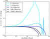Fig. 1. Right-hand side of Eq. (1) evaluated on the GENEC models at zero metallicity and indicated accretion rates. The grey line indicates the zero.

Fig. 2. Right-hand side of Eq. (11) for the same models as in Fig. 1.

The reliability of these two contradictory results can be tested by looking at the terms of the sum individually, namely, the integrals I_i and J_i. Figure 3 shows these integrals in absolute values for the GENEC model at zero metallicity and Ṁ = 10 M_⊙ yr⁻¹. The knee in the integrals near log M/M_⊙ = 4.3 indicates the beginning of H-burning. Integrals I₃ = J₃ and I₄ = J₄ always remain negligible compared to the others, and their role in the GR instability is still weakened by the fact that they have opposite signs and similar magnitudes. The stability of the star depends mainly on the balance between the stabilising integral I₁ > 0 (or J₁ > 0), which reflects the departures from the Eddington limit, and the destabilising integral I₂ < 0 (or J₂ < 0), which reflects the departures from the Newtonian limit. We see that I₁ and I₂ are indeed very close, as is expected for post-Newtonian stars near the Eddington limit. But the fact that the differences remain invisible on a logarithmic scale indicates that the relative differences are negligible. Thus, any numerical noise that would not affect the equilibrium properties could, in fact, hinder the dynamical effects. It shows how difficult it is to capture the GR instability simply by accounting for GR hydrodynamics in numerical models, even if these models satisfy the equations of structures with a high level of precision. In contrast, if we compare J₁ and J₂, we see that they differ by orders of magnitude during most of the run. The point at which they cross each other is clearly recognisable and they do not suffer from the small numerical variations in the integrals, which shows the high level of accuracy for this method.

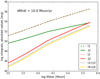Fig. 3. Absolute values of the integrals ((3)–(4), dashed lines) and ((12)–(15), solid lines) for the GENEC model at zero metallicity with the indicated rate. The green curves are the stabilising integrals I1, J1 > 0, while the red curves are the destabilising integrals I2, J2 < 0. The grey curves are I3 > 0 and I4 < 0, that remain negligible, and unchanged between Eqs. (1) and (11).

The final masses obtained in this way with the GENEC models are summarised in Table 1. When the model does not reach the instability at the end of the run, we indicate the last value for the mass that is reached and set it as a lower limit. The model at 0.1 M_⊙ yr⁻¹ and zero metallicity is not shown; its mass at the end of the run is 70 000 M_⊙, which is far from instability (Fig. 2). We confirm that increasing the accretion rate allows us to reach higher masses before the instability. However, we see that for Ṁ ≤ 10 M_⊙ yr⁻¹ and Z = 0, the stellar mass cannot exceed 500 000 M_⊙. Masses above this limit require rates of ≳100−1000 M_⊙ yr⁻¹or the presence of metals. The most massive stable model we obtained is the one at solar metallicity and 1000 M_⊙ yr⁻¹, where the GR instability develops only at 759 000 M_⊙. Interestingly, an extrapolation of the curve of the 1000 M_⊙ yr⁻¹ model at zero metallicity in Fig. 2 suggests a final mass > 10⁶ M_⊙.

4. Discussion

Two prior studies have addressed the question of the final mass of Population III SMSs accreting at the rates of atomically cooled halos (Umeda et al. 2016; Woods et al. 2017). These works were based on stellar evolution models that account for hydrodymamics numerically, based on assumptions of spherical symmetry and post-Newtonian corrections. The only ingredient that accounts for GR in these studies is the correction to the equation of radial momentum, following Fuller et al. (1986). With this method, the GR hydrodynamics is treated only numerically, by adding small corrections to the intrinsically stable Newtonian structures. In spite of the identical physical ingredients, these two studies obtained very different results, particularly with regard to the rates > 1 and the origin of these discrepancies is not understood (Woods et al. 2019). The final masses obtained in these simulations are shown in Fig. 4 as a function of the accretion rate. As discussed in Woods et al. (2019), the final mass of the 10 M_⊙ yr⁻¹ model differs by a factor of > 2 between both studies. It is thought that at least part of this discrepancy is the result of the differences that appear in the hydrostatic structures themselves since Woods et al. (2017) was able to obtain much larger convective cores than Umeda et al. (2016). However, this statement is speculative and, moreover, the origin of the differences in the structure are not better understood.

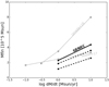Fig. 4. Final masses of SMSs at zero metallicity, accreting at the rates of atomically cooled halos. The results of the present work are shown by a solid black line. The masses obtained with the polytropic criterion are shown as dashed lines when applied in the whole star (lower line) and in the convective core only (upper line). The results of Umeda et al. (2016) and Woods et al. (2017), obtained with numerical hydrodynamics, are shown in grey.

The GENEC models of Haemmerlé et al. (2018, 2019) used in the present work were computed with exactly the same ingredients as in Umeda et al. (2016) and Woods et al. (2017), except for the hydrodynamics, which is missing. With regard to the structures, these models are in very good agreement with Umeda et al. (2016), as well as with Hosokawa et al. (2013) who consider lower masses. It allows for a direct comparison between our results, which account for hydrodynamics ab initio, and the results of Umeda et al. (2016), which account for hydrodynamics based on numerical methods. To that aim, we plotted in Fig. 4 the final masses of the GENEC models at zero metallicity and Ṁ = 1−10 M_⊙ yr⁻¹. The comparison cannot be done for 0.1 M_⊙ yr⁻¹, as the GENEC run at this rate does not cover the full evolution, due to numerical instability (Sect. 3). We see that in spite of the fact that our structures are identical to those of Umeda et al. (2016), our final masses remain much closer to those of Woods et al. (2017). For 10 M_⊙ yr⁻¹, our final mass exceeds that of Woods et al. (2017) only by ∼30%, while a factor of 2 remains in the final mass of Umeda et al. (2016). This discrepancy clearly reveals that the differences in the size of the convective core between Umeda et al. (2016) and Woods et al. (2017) account for the negligible part in the discrepancies in the final mass and that these discrepancies are essentially attributed to the numerical treatment of hydrodynamics. In view of the difficulties involved in capturing small post-Newtonian corrections in numerical models (Sect. 3), the numerical noise in hydrodynamical simulations appears as the most natural suspect for the discrepancies, of a factor of 2, in the final mass.

We also indicate, in Fig. 4, the final masses obtained with the polytropic criterion of Chandrasekhar (1964) applied to the GENEC models, in the star as a whole (lower dashed line) and in the convective core only (upper dashed line). This confirms that the use of the polytropic criterion leads to an underestimation of the final mass, as was already pointed out by Woods et al. (2017). Thus, the present method appears as the most consistent, accurate, and straightforward in its practical application.

5. Summary and conclusions

In this work, we demonstrate how the GR instability can be captured ab initio with a high level of accuracy in numerical hydrostatic stellar models, which allows for reliable determination of the final mass of accreting SMSs in a simpler and more consistant way than numerical hydrodynamics. We emphasise that our treatment of the instability relies directly on the general expression of the relativistic pulsation equation of Chandrasekhar (1964), without any additional assumption. According to our results, the mass of spherical Population III SMSs accreting at the rates of atomically cooled halos always remains < 500 000 M_⊙. Larger masses can be reached only for rates ≳100−1000 M_⊙ yr⁻¹or in the case of non-primordial chemical composition. For conditions of galaxy mergers (Mayer & Bonoli 2019; Haemmerlé et al. 2019), masses ∼10⁶ M_⊙ could be reached. Our method can be used to check the consistency of the numerical treatment of GR hydrodynamics in stellar evolution codes.

Acknowledgments

LH has received funding from the European Research Council (ERC) under the European Union’s Horizon 2020 research and innovation programme (grant agreement No 833925, project STAREX).

References

All Tables

All Figures

	Fig. 1. Right-hand side of Eq. (1) evaluated on the GENEC models at zero metallicity and indicated accretion rates. The grey line indicates the zero.
In the text

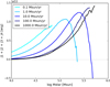	Fig. 2. Right-hand side of Eq. (11) for the same models as in Fig. 1.
In the text

	Fig. 3. Absolute values of the integrals ((3)–(4), dashed lines) and ((12)–(15), solid lines) for the GENEC model at zero metallicity with the indicated rate. The green curves are the stabilising integrals I1, J1 > 0, while the red curves are the destabilising integrals I2, J2 < 0. The grey curves are I3 > 0 and I4 < 0, that remain negligible, and unchanged between Eqs. (1) and (11).
In the text

Fig. 4. Final masses of SMSs at zero metallicity, accreting at the rates of atomically cooled halos. The results of the present work are shown by a solid black line. The masses obtained with the polytropic criterion are shown as dashed lines when applied in the whole star (lower line) and in the convective core only (upper line). The results of Umeda et al. (2016) and Woods et al. (2017), obtained with numerical hydrodynamics, are shown in grey.

In the text

References

- Bromm, V., & Loeb, A. 2003, ApJ, 596, 34 [NASA ADS] [CrossRef] [Google Scholar]
- Chandrasekhar, S. 1964, ApJ, 140, 417 [NASA ADS] [CrossRef] [MathSciNet] [Google Scholar]
- Fuller, G. M., Woosley, S. E., & Weaver, T. A. 1986, ApJ, 307, 675 [NASA ADS] [CrossRef] [Google Scholar]
- Haemmerlé, L., Woods, T. E., Klessen, R. S., Heger, A., & Whalen, D. J. 2018, MNRAS, 474, 2757 [NASA ADS] [CrossRef] [Google Scholar]
- Haemmerlé, L., Meynet, G., Mayer, L., et al. 2019, A&A, 632, L2 [CrossRef] [EDP Sciences] [Google Scholar]
- Haemmerlé, L., Mayer, L., Klessen, R. S., et al. 2020, Space Sci. Rev., 216, 48 [CrossRef] [Google Scholar]
- Hosokawa, T., Yorke, H. W., Inayoshi, K., Omukai, K., & Yoshida, N. 2013, ApJ, 778, 178 [NASA ADS] [CrossRef] [Google Scholar]
- Latif, M. A., Schleicher, D. R. G., Schmidt, W., & Niemeyer, J. C. 2013, MNRAS, 436, 2989 [NASA ADS] [CrossRef] [Google Scholar]
- Mayer, L., & Bonoli, S. 2019, Rep. Prog. Phys., 82, 016901 [Google Scholar]
- Mayer, L., Kazantzidis, S., Escala, A., & Callegari, S. 2010, Nature, 466, 1082 [NASA ADS] [CrossRef] [Google Scholar]
- Mayer, L., Fiacconi, D., Bonoli, S., et al. 2015, ApJ, 810, 51 [NASA ADS] [CrossRef] [Google Scholar]
- Regan, J. A., Visbal, E., Wise, J. H., et al. 2017, Nat. Astron., 1, 0075 [CrossRef] [Google Scholar]
- Sakurai, Y., Hosokawa, T., Yoshida, N., & Yorke, H. W. 2015, MNRAS, 452, 755 [NASA ADS] [CrossRef] [Google Scholar]
- Umeda, H., Hosokawa, T., Omukai, K., & Yoshida, N. 2016, ApJ, 830, L34 [NASA ADS] [CrossRef] [Google Scholar]
- Woods, T. E., Heger, A., Whalen, D. J., Haemmerlé, L., & Klessen, R. S. 2017, ApJ, 842, L6 [NASA ADS] [CrossRef] [Google Scholar]
- Woods, T. E., Agarwal, B., Bromm, V., et al. 2019, PASA, 36, e027 [NASA ADS] [CrossRef] [Google Scholar]
All Tables
Stellar mass (in 105 M⊙) at the onset of GR instability for the GENEC models at the indicated metallicities and accretion rates.